Equation Chapter 1 Section 1
Abstract—When performing predictive data mining, the use of ensembles is known to increase prediction accuracy, compared to single models. To obtain this higher accuracy, ensembles should be built from base classifiers that are both accurate and diverse. The question of how to balance these two properties in order to maximize ensemble accuracy is, however, far from solved and many different techniques for obtaining ensemble diversity exist. One such technique is bagging, where implicit diversity is introduced by training base classifiers on different subsets of available data instances, thus resulting in less accurate, but diverse base classifiers. In this paper, genetic programming is used as an alternative method to obtain implicit diversity in ensembles by evolving accurate, but different base classifiers in the form of decision trees, thus exploiting the inherent inconsistency of genetic programming. The experiments show that the GP approach outperforms standard bagging of decision trees, obtaining significantly higher ensemble accuracy over 25 UCI datasets. This superior performance stems from base classifiers having both higher average accuracy and more diversity. Implicitly introducing diversity using GP thus works very well, since evolved base classifiers tend to be highly accurate and diverse.
I. INTRODUCTION
PREDICTIVE data mining deals with the problem of estimating the value of a target variable based on a number of input variables (attributes). If the target variable is continuous, the task is called regression and if it is categorical, the task is termed classification. Models are typically constructed by using some statistical or machine learning technique on a set of training data, where values for the target variable are known, and the model then learns a function from the input vector to the target variable.
The aim is to produce models that perform well on unseen data, i.e. models with high predictive accuracy. Many different techniques for producing such models exist, with transparent models being preferred when models need to be interpretable or comprehensible. Among transparent models, decision trees are the most commonly used representation and a wealth of powerful decision tree algorithms exist, e.g. C4.5/C5.0 [1] and CART [2]. Opaque models include artificial neural networks (ANNs) and support vector machines (SVMs). Whether using transparent or opaque models, it is a known fact that predictive accuracy can be increased by using ensembles, i.e. composite models consisting of aggregated multiple models, called base models, each constructed separately. Ensembles can be All authors are with the School of Business and Informatics, University of Borås, SE-50190 Borås, Sweden. Email: {ulf.johansson, cecilia.sonstrod,
created from virtually any kind of model, e.g. decision trees or ANNs. Successful ensembles rely on the fact that the base classifiers make different and most desirably independent errors, so that averaging predictions will eliminate these errors. It is thus important to obtain ensembles with some diversity, i.e. where base classifiers make their errors on different instances.
When constructing ensembles, the two most important choices are how to construct the base models and how to combine predictions from the base models. When using a deterministic machine learning technique (for instance C5.0 decision trees) to create the base models, diversity must somehow be introduced into the ensemble by obtaining different base models from the same dataset. One such technique is bootstrap aggregating, more commonly known as bagging, introduced by Breiman in [3], where base models in an ensemble are trained using slightly different parts of the available training data.
GP has in many studies proved to be a very efficient search strategy for data mining problems. Often, GP results are comparable to, or even better than, results obtained by more specialized machine learning techniques. One example is when GP is used for classification, and the performance is compared to decision tree algorithms or rule inducers. Specifically, several studies show that decision trees evolved using GP often are more accurate than trees induced by standard techniques like C4.5/C5.0 and CART; see e.g. [4] and [5]. The main reason for this is that GP is a global optimization technique, while decision tree algorithms typically choose splits greedily, working from the root node down. Informally, this means that GP often will make some locally sub-optimal splits, but the overall model will still be more accurate and more general.
Often, however, the inherent inconsistency (i.e. that runs on the same data using identical settings can produce different results) of GP is cited as a disadvantage for data mining applications, based on the argument that decision-makers want to understand models and that several different models from the same data are confusing. But, when building ensembles, GP inconsistency can be utilized to obtain diverse ensembles, thus increasing predictive accuracy. The main purpose of this study is therefore to build ensembles of decision trees generated by GP, and compare these, regarding both predictive accuracy and diversity, to ensembles created using standard bagging.
Using Genetic Programming to Obtain Implicit Diversity
Ulf Johansson, Cecilia Sönströd, Tuve Löfström and Rikard König
II. BACKGROUND
An ensemble is a composite model aggregating multiple base models, so the ensemble prediction, when applied to a novel instance, is a function of all included base models. Ensemble learning, consequently, refers to a large collection of methods that learn a target function by training a number of individual learners and combining their predictions.
The most intuitive explanation for why ensembles work is that combining several models using averaging will eliminate uncorrelated base classifier errors; see e.g. [6]. Naturally, this requires that base classifiers commit their errors on different instances – there is nothing to gain by combining identical models. Informally, the key term diversity therefore means that the base classifiers make their mistakes on different instances. The important result that ensemble error depends not only on the average accuracy of the base models but also on their diversity1 was formally derived by Krogh and Vedelsby in [7]. Based on this, the overall goal when creating ensembles is to combine models that are highly accurate, but differ in their predictions. Unfortunately, base classifier accuracy and diversity is highly correlated, so maximizing diversity would most likely reduce the average accuracy. In addition, diversity is, for predictive classification, not uniquely defined. Because of this, several different diversity measures have been suggested, and to further complicate matters, no specific diversity measure has shown high correlation with accuracy on novel data. As mentioned above, Krogh and Vedelsby derived an equation stating that the generalization ability of an ensemble is determined by the average generalization ability and the average diversity (ambiguity) of the individual models in the ensemble. More specifically; the ensemble error, E, can be expressed as:
E=E−A (1) whereEis the average error of the base models andAis the ensemble diversity, measured as the weighted average of the squared differences in the predictions of the base models and the ensemble. In a regression context and using averaging to combine predictions, this is equivalent to:
2 1 2 1 2 ˆ ˆ ˆ ˆ ( ens ) ( i ) ( i ens) i i E Y Y Y Y Y Y M M = − =
∑
− −∑
− (2)So, the error of the ensemble is guaranteed to be less than or equal to the average error of the base models. The first term is the (possibly weighted) average of the individual classifiers and the second is the diversity term; i.e. the amount of variability among ensemble members. Since diversity is always positive, this decomposition proves that the ensemble will always have higher accuracy than the average accuracy obtained by the individual classifiers. The problem is, however, the fact that the two terms are
1 Krogh and Vedelsby used the term ambiguity instead of
diversity in their paper. In this paper, the more common term diversity is, however, used exclusively.
normally highly correlated, making it necessary to balance them rather than just maximize diversity.
By relating this to the bias-variance decomposition and assuming that the ensemble is a convex combined ensemble (e.g. using averaging), a bias-variance-covariance decomposition can be obtained for the ensemble MSE; see (3) below.
( )
2
2 1 1
ˆ
( ens ) var 1 covar
E Y Y bias
M M
= − = + + − (3)
From this it is evident that the error of the ensemble depends critically on the amount of correlation between models, quantified in the covariance term. Ideally, the covariance should be minimized, without causing changes in the bias or variance terms.
When discussing ensembles in a classification context, it should be noted that unless classification is handled like an instance of regression (i.e. the outputs are ordinal and typically represent probabilities) the framework described above does not apply. When the predictors are only able to output a class label, the outputs have no intrinsic ordinality between them, thus making the concept of covariance undefined. Using a zero-one loss function, there is no clear analogy to the bias-variance-covariance decomposition. So, obtaining an expression where the classification error is decomposed into error rates of the individual classifiers and a diversity term is currently beyond the state of the art. Instead, methods typically use heuristic expressions that try to approximate the unknown diversity term.
So, the question of how to balance base classifier accuracy against diversity is far from solved and it is furthermore not even evident how to measure diversity. When the task is classification, it is obvious to search for a diversity measure well correlated with majority voting. Unfortunately, no such measure has been found, despite extensive experimentation [8]. For example, in [9], ten different diversity measures were evaluated on binary classifier outputs; i.e. correct or incorrect vote for the correct class. The main result was that all diversity measures showed low or very low correlation with test set accuracy. Despite this, diversity has been experimentally shown to be beneficial when building classification ensembles.
In this study, the two diversity measures used were disagreement and double fault, both based on pair-wise comparisons between all base classifiers in the ensemble. The output of each base model Di is represented as an
N-dimensional binary vector yi, where yi,j=1 if Di correctly
classifies instance zj and 0 otherwise. For pair-wise
comparison, the notation Nab then means the number of instances for which yj,i= a and yj,k = b. For example, N
11
is the number of instances correctly classified by both base classifiers.
Disagreement is the ratio between the number of instances on which one classifier is correct and the other incorrect to the total number of instances, and is thus calculated using:
01 10 , 11 10 01 00 i k N N Dis N N N N = + +
+
+
(4) Double fault is the proportion of instances misclassified by both classifiers: 00 , 11 10 01 00 i k N DF N N N N = + + + (5) For an ensemble consisting of L classifiers, the averaged diversity (i.e. disagreement or double fault), D, over all pairs of classifiers is: 1 , 1 1 2 ( 1) L L av i k i k i D D L L − = = + = −∑ ∑
(6) Bagging obtains diversity by using resampling to create different training sets for each base classifier; each training set has the same size as the original training set, but will contain multiple copies of some instances and lack other instances. The implicit diversity thus introduced by bagging, by giving base classifiers access only to a subset of the available training data, will result in weaker (i.e. lower prediction accuracy) base classifiers than if they were trained using all available training data. Another method that introduces diversity implicitly is random forests [10], using randomness in both feature and instance selection for base classifiers. Successful as these approaches are, it is important to remember that introducing diversity by limiting the capability of the base classifiers to model the whole data set will generally result in lower base classifier accuracy. It is not obvious that introducing diversity by deliberately weakening the base classifiers is the best way to handle the trade-off between base classifier accuracy and diversity in order to obtain high ensemble accuracy.A different approach is to utilize an indeterministic technique for the base classifier construction, and thus introduce implicit diversity by building each base classifier model, still using all available training data. For example, if ANNs are used as base classifiers, using different architectures or even just randomizing initial weights will result in some diversity among base classifiers. Obviously, the key to this approach is that the indeterministic technique is capable of producing accurate and sufficiently diverse models.
G-REX is a general data mining framework based on GP; see [11], originally designed as a rule extraction tool [12]. One key property of G-REX is the ability to use a variety of different representation languages, just by choosing suitable function and terminal sets, and specifying a BNF-style grammar. G-REX has previously been used for both rule extraction (from opaque models) and rule induction (directly on data), using, for instance, decision trees, regression trees, Boolean rules and fuzzy rules. For a summary of the G-REX technique and previous studies, see [13].
For predictive modeling, the fitness function is usually based on accuracy in some way, and there is also the option
of including a length penalty to encourage shorter representations, either to increase comprehensibility or to avoid over-fitting.
III. METHOD
All experiments were conducted using the data mining workbench WEKA [14]. Ensembles of three different decision trees using WEKA’s bagging option were used for comparison.
A. Techniques
The chosen techniques were J48 (the WEKA C4.5 implementation) and REPTree, which is the default choice of base classifier for bagging in WEKA. The motivation for using J48 trees is that they represent the state-of-the-art decision trees. REPTree is an efficient decision tree algorithm that uses information gain and reduced-error pruning to build trees. Since no calculation of diversity measures is included in WEKA, this was added along with calculation of base classifier accuracy, without modifying the model construction.
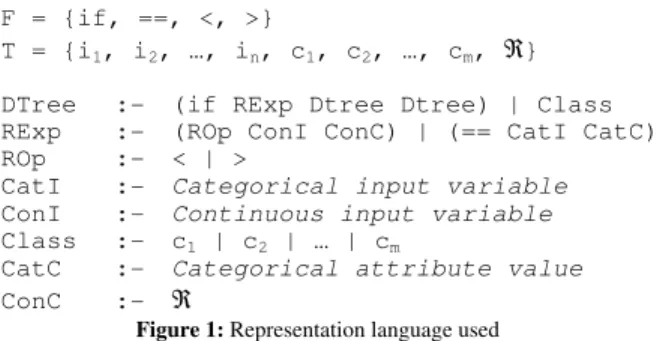
For the GP ensembles, decision trees built by rule induction with G-REX were used as base models, using a grammar similar to standard decision trees, shown in Figure 1 below. The sets F and T describe the available functions and terminals, respectively. Here, the functions used are an if-statement and three relational operators. The terminals are attributes from the data set and random real numbers.
F = {if, ==, <, >}
T = {i1, i2, …, in, c1, c2, …, cm, ℜ}
DTree :- (if RExp Dtree Dtree) | Class RExp :- (ROp ConI ConC) | (== CatI CatC) ROp :- < | >
CatI :- Categorical input variable ConI :- Continuous input variable Class :- c1 | c2 | … | cm
CatC :- Categorical attribute value ConC :- ℜ
Figure 1: Representation language used
The GP settings used for generating base models are given in Table I below.
TABLE I GP PARAMETER SETTINGS Parameter Value Crossover rate 0.9 Mutation rate 0.01 Population size 800 Generations 50 Creation depth 8
Creation method Ramped half-and-half Fitness function Accuracy - length penalty
Selection Roulette wheel
B. Data sets
The 25 datasets used are all publicly available from the UCI Repository [15]. For a summary of dataset characteristics see Table II below. Instances is the total number of instances in the dataset. Classes is the number of output classes in the dataset. Cont. is the number of continuous input variables and Cat. is the number of categorical input variables.
TABLE II DATASET CHARACTERISTICS
Dataset Instances Classes Cont. Cat.
Breast cancer 286 2 0 9 CMC 1473 3 2 7 Credit-A 690 2 6 9 Cylinder 540 2 18 21 Diabetes-Pima 768 2 8 0 E-coli 336 8 7 0 Haberman 306 2 3 0 Heart-Cleve 303 2 6 7 Heart-Hungarian 294 2 6 7 Heart-Statlog 270 2 6 7 Hepatitis 155 2 6 13 Iono 351 2 34 0 Iris 150 3 4 0 Labor 57 2 8 8 Liver-Bupa 345 2 6 0 Lymph 148 4 3 15 Sick 2800 2 7 22 Sonar 208 2 60 0 TAE 151 3 1 4 Tic-Tac-Toe 958 2 0 9 Vehicle 846 4 18 0 Vote 435 2 0 16 Wine 178 3 13 0
Wisconsin breast cancer (WBC) 699 2 9 0
Zoo 100 7 0 16
C. Experiments
For all experimentation, 4-fold cross validation was used. 9 base classifiers were bagged for all techniques, and WEKA’s averaging mechanism for ensemble voting was used when combining the base models.
IV. RESULTS
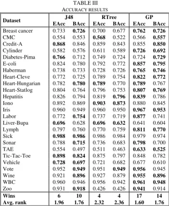
In Table III below, the results regarding accuracy are shown, where EAcc stands for ensemble accuracy and BAcc stands for average base classifier accuracy. All accuracies are averaged over the 4 folds.
TABLE III ACCURACY RESULTS
Dataset J48 RTree GP
EAcc BAcc EAcc BAcc EAcc BAcc
Breast cancer 0.733 0.726 0.700 0.677 0.762 0.726 CMC 0.554 0.553 0.568 0.522 0.566 0.557 Credit-A 0.868 0.846 0.859 0.843 0.855 0.850 Cylinder 0.582 0.576 0.611 0.589 0.726 0.692 Diabetes-Pima 0.766 0.712 0.749 0.724 0.724 0.729 E-coli 0.824 0.780 0.792 0.772 0.857 0.795 Haberman 0.738 0.733 0.728 0.726 0.765 0.746 Heart-Cleve 0.772 0.725 0.789 0.754 0.822 0.772 Heart-Hungarian 0.782 0.780 0.789 0.770 0.789 0.767 Heart-Statlog 0.804 0.764 0.796 0.753 0.807 0.769 Hepatitis 0.826 0.794 0.819 0.796 0.839 0.786 Iono 0.892 0.869 0.903 0.873 0.880 0.845 Iris 0.960 0.949 0.960 0.950 0.967 0.953 Labor 0.772 0.754 0.737 0.719 0.877 0.741 Liver-Bupa 0.696 0.628 0.696 0.632 0.641 0.604 Lymph 0.797 0.760 0.770 0.759 0.811 0.770 Sick 0.988 0.986 0.986 0.984 0.979 0.974 Sonar 0.788 0.715 0.736 0.683 0.798 0.700 TAE 0.554 0.497 0.511 0.463 0.633 0.525 Tic-Tac-Toe 0.898 0.824 0.875 0.797 0.848 0.782 Vehicle 0.728 0.697 0.721 0.682 0.677 0.610 Vote 0.952 0.949 0.951 0.949 0.956 0.945 Wine 0.921 0.896 0.927 0.879 0.955 0.896 WBC 0.960 0.946 0.956 0.942 0.961 0.948 Zoo 0.931 0.918 0.426 0.426 0.941 0.914 Wins 6 10 4 4 17 14 Avg. rank 1.96 1.76 2.32 2.36 1.60 1.76
The most obvious result is that GP is in a class of its own, winning more than two-thirds of all datasets. Performing a direct comparison between GP and J48, where GP wins 18 out of 25 datasets, a one-tailed sign test with 25 datasets gives a p-value of 0.022, thus indicating a significant difference between the two techniques at α = 0.05. Performing the same pair-wise test against REPTrees, the numbers are 16 wins and 1 draw for GP, resulting in a
p-value of 0.076, i.e. significant at α = 0.10, but not at α =
0.05. However, one more win would suffice to obtain significance at α = 0.05. Regarding base classifier accuracy, GP wins a majority of the datasets, and J48 also performs well. The reason for GP obtaining the most accurate base classifiers is most likely that each GP base classifier has access to all training data, while J48 and REPTrees have to use bootstraps.
Some interesting observations can be made when comparing ensemble and base classifier accuracies. Although high base classifier accuracy is obviously important for ensemble accuracy, it is striking that for as many as nine datasets, the winning technique does not have the highest average base classifier accuracy. Looking at the different techniques from this perspective, GP obtains the highest base classifier accuracy on only 11 of its winning datasets, indicating that good base classifier performance is only part of the explanation for the superior ensemble accuracies. For J48, it is notable that having the highest average base classifier accuracy only leads to the highest ensemble accuracy on 3 out of 10 datasets.
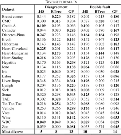
Table IV shows diversity results for all techniques. Note that for disagreement, a high value indicates more diverse base classifiers, but that for double fault, a low value means more diversity.
TABLE IV
DIVERSITY RESULTS
Dataset Disagreement Double fault J48 RTree GP J48 RTree GP Breast cancer 0.144 0.220 0.187 0.202 0.213 0.180 CMC 0.300 0.315 0.204 0.327 0.320 0.342 Credit-A 0.109 0.103 0.066 0.100 0.105 0.117 Cylinder 0.044 0.080 0.283 0.402 0.370 0.167 Diabetes-Pima 0.247 0.223 0.146 0.164 0.164 0.198 E-coli 0.136 0.122 0.164 0.152 0.167 0.123 Haberman 0.143 0.145 0.142 0.196 0.202 0.183 Heart-Cleveland 0.225 0.201 0.224 0.145 0.146 0.117 Heart-Hungarian 0.134 0.173 0.171 0.154 0.144 0.148 Heart-Statlog 0.216 0.209 0.203 0.128 0.143 0.130 Hepatitis 0.170 0.163 0.208 0.121 0.123 0.110 Iono 0.134 0.116 0.138 0.064 0.068 0.086 Iris 0.023 0.040 0.037 0.040 0.030 0.028 Labor 0.177 0.252 0.326 0.157 0.154 0.096 Liver-Bupa 0.348 0.334 0.361 0.198 0.200 0.215 Lymph 0.204 0.136 0.220 0.138 0.173 0.120 Sick 0.012 0.013 0.018 0.008 0.009 0.017 Sonar 0.320 0.298 0.343 0.125 0.168 0.128 TAE 0.302 0.328 0.320 0.352 0.373 0.314 Tic-Tac-Toe 0.216 0.254 0.239 0.068 0.080 0.098 Vehicle 0.253 0.266 0.288 0.176 0.184 0.246 Vote 0.014 0.012 0.043 0.043 0.045 0.034 Wine 0.110 0.131 0.142 0.048 0.056 0.033 WBC 0.049 0.049 0.046 0.029 0.034 0.029 Zoo 0.059 0.000 0.081 0.053 0.574 0.045 Most diverse 5 8 13 10 3 14
As seen in the table, there is a quite clear ordering for disagreement, with GP getting the highest disagreement, followed by REPTree and then J48. When comparing the disagreement results to the accuracy results in Table III, a rather clear picture emerges, especially for J48. On all seven datasets where J48 fails to obtain the highest ensemble accuracy, despite having the highest average base classifier accuracy, it has significantly lower disagreement than GP. This indicates that it is often the case that when J48 has highly accurate base classifiers, they tend to be too homogenous to serve well together as base classifiers in an ensemble.
Using double fault, both GP and J48 obtain much higher diversity than REPTree, which is partly explained by their superior base classifiers. It is remarkable to note the strong correlation between double fault and ensemble accuracy; on all but three datasets, the technique with the lowest double fault value emerges as ensemble accuracy winner. Looking at how the three techniques rank on different measures, the correlation between double fault and ensemble accuracy is, in this study, actually much stronger than between base classifier accuracy and ensemble accuracy, or, for that matter, between base classifier accuracy and double fault.
V. CONCLUSIONS
In this study, GP has been used for tree induction in order to achieve implicit diversity between base classifiers in ensemble models. This approach contrasts with the established bagging technique, which seeks to obtain diversity among the base classifiers in an ensemble by training them on different subsets of the data, thus resulting in weaker models being used for building the ensemble. The aim was to investigate whether GP could obtain sufficiently more accurate base classifiers than bagging, and also carry this advantage over to ensemble accuracy. Since diversity is known to be beneficial for ensemble construction, the intention was also to analyze diversity in ensembles created by GP and to compare this against the diversity obtained when using standard bagging.
Most importantly, the experimental results show that ensembles of trees evolved by GP perform significantly better regarding accuracy than ensembles constructed by bagging decision trees built with C4.5 or reduced error- pruning. Interestingly enough, the superior performance of GP is due to both the higher base classifier accuracies and the higher diversity achieved.
The generally higher base classifier accuracies are explained by each base classifier being built using all available training data. The fact that the inherent inconsistency of GP actually produced more implicit diversity than bagging was, on the other hand, somewhat unexpected. This result, together with the highly accurate base classifiers is, however, a very strong argument for the use of GP in ensemble creation.
An interesting observation is that diversity, measured as double fault, had a very strong impact on ensemble accuracy. As a matter of fact, the technique obtaining the lowest double fault value also had the highest ensemble accuracy on 22 of 25 datasets.
Overall, the experiments indicate that standard bagging often may result in base models being either too weak, or too homogenous, and that GP could contribute to ensemble creation techniques by providing highly accuracy, but still diverse base models.
VI. FUTURE WORK
The fact that GP was able to obtain diversity more or less “for free” makes it an interesting alternative also for other ensemble designs. Using an evolutionary approach for boosting actually has another attractive property, since the strategy that harder instances (instances where many base models fail) should be prioritized, could be implemented quite straightforwardly in the GP fitness function. With this in mind, we will, in a future study, investigate if evolved base classifiers could be successfully boosted.
REFERENCES
[1] J. R. Quinlan. C4.5: Programs for Machine Learning, Morgan Kaufmann, 1993.
[2] L. Breiman. J. H. Friedman. R. A. Olshen and C. J. Stone.
Classification and Regression Trees. Wadsworth International. 1984.
[3] L. Breiman, Bagging Predictors, Machine Learning, 24(2): 123-140, 1996.
[4] A. Tsakonas, A comparison of classification accuracy of four genetic programming-evolved intelligent structures, Information Sciences, 176(6): 691-724, 2006.
[5] C. C. Bojarczuk, H. S. Lopes and A. A. Freitas, Data Mining with Constrained-syntax Genetic Programming: Applications in Medical Data Sets, Intelligent Data Analysis in Medicine and Pharmacology -
a workshop at MedInfo-2001, 2001.
[6] T. G. Dietterich, Machine learning research: four current directions,
The AI Magazine, 18: 97-136, 1997.
[7] A. Krogh and J. Vedelsby, Neural network ensembles, cross validation, and active learning. Advances in Neural Information
Processing Systems, Volume 2:650-659, San Mateo, CA, Morgan
Kaufmann, 1995.
[8] G. Brown, J. Wyatt, R. Harris and X. Yao, Diversity Creation Methods: A Survey and Categorisation, Journal of Information
Fusion, 6(1): 5-20, 2005.
[9] L. I. Kuncheva and C. J. Whittaker, Measures of Diversity in Classifier Ensembles and Their Relationship with the Ensemble Accuracy, Machine Learning, (51):181-207, 2003.
[10] L. Breiman, Random Forests, Machine Learning, 45(1): 5-32, 2001. [11] R. König, U. Johansson and L. Niklasson, G-REX: A Versatile
Framework for Evolutionary Data Mining, IEEE International
Conference on Data Mining (ICDM08), Demo paper, Workshop
proceedings, pp. 971-974, 2008.
[12] U. Johansson, R. König and L. Niklasson, Rule Extraction from Trained Neural Networks using Genetic Programming, 13th International Conference on Artificial Neural Networks, Istanbul,
Turkey, supplementary proceedings pp. 13-16, 2003.
[13] U. Johansson, Obtaining accurate and comprehensible data mining
models: An evolutionary approach, PhD thesis, Institute of
Technology, Linköping University, 2007.
[14] I. H. Witten and E. Frank: Data Mining – Machine Learning Tools
and Techniques, 2nd ed, Morgan Kaufman, 2005.
[15] A. Asuncion and D. J. Newman, UCI machine learning repository, 2007.