ScienceDirect
Available online at Available online at www.sciencedirect.comwww.sciencedirect.com
ScienceDirect
Energy Procedia 00 (2017) 000–000
www.elsevier.com/locate/procedia
1876-6102 © 2017 The Authors. Published by Elsevier Ltd.
Peer-review under responsibility of the Scientific Committee of The 15th International Symposium on District Heating and Cooling.
The 15th International Symposium on District Heating and Cooling
Assessing the feasibility of using the heat demand-outdoor
temperature function for a long-term district heat demand forecast
I. Andrić
a,b,c*, A. Pina
a, P. Ferrão
a, J. Fournier
b., B. Lacarrière
c, O. Le Corre
caIN+ Center for Innovation, Technology and Policy Research - Instituto Superior Técnico, Av. Rovisco Pais 1, 1049-001 Lisbon, Portugal bVeolia Recherche & Innovation, 291 Avenue Dreyfous Daniel, 78520 Limay, France
cDépartement Systèmes Énergétiques et Environnement - IMT Atlantique, 4 rue Alfred Kastler, 44300 Nantes, France
Abstract
District heating networks are commonly addressed in the literature as one of the most effective solutions for decreasing the greenhouse gas emissions from the building sector. These systems require high investments which are returned through the heat sales. Due to the changed climate conditions and building renovation policies, heat demand in the future could decrease, prolonging the investment return period.
The main scope of this paper is to assess the feasibility of using the heat demand – outdoor temperature function for heat demand forecast. The district of Alvalade, located in Lisbon (Portugal), was used as a case study. The district is consisted of 665 buildings that vary in both construction period and typology. Three weather scenarios (low, medium, high) and three district renovation scenarios were developed (shallow, intermediate, deep). To estimate the error, obtained heat demand values were compared with results from a dynamic heat demand model, previously developed and validated by the authors.
The results showed that when only weather change is considered, the margin of error could be acceptable for some applications (the error in annual demand was lower than 20% for all weather scenarios considered). However, after introducing renovation scenarios, the error value increased up to 59.5% (depending on the weather and renovation scenarios combination considered). The value of slope coefficient increased on average within the range of 3.8% up to 8% per decade, that corresponds to the decrease in the number of heating hours of 22-139h during the heating season (depending on the combination of weather and renovation scenarios considered). On the other hand, function intercept increased for 7.8-12.7% per decade (depending on the coupled scenarios). The values suggested could be used to modify the function parameters for the scenarios considered, and improve the accuracy of heat demand estimations.
© 2017 The Authors. Published by Elsevier Ltd.
Peer-review under responsibility of the Scientific Committee of The 15th International Symposium on District Heating and Cooling.
Keywords: Heat demand; Forecast; Climate change
Energy Procedia 142 (2017) 1721–1727
1876-6102 © 2017 The Authors. Published by Elsevier Ltd.
Peer-review under responsibility of the scientific committee of the 9th International Conference on Applied Energy . 10.1016/j.egypro.2017.12.555
ScienceDirect
Energy Procedia 00 (2017) 000–000www.elsevier.com/locate/procedia
1876-6102 © 2017 The Authors. Published by Elsevier Ltd.
Peer-review under responsibility of the scientific committee of the 9th International Conference on Applied Energy.
9th International Conference on Applied Energy, ICAE2017, 21-24 August 2017, Cardiff, UK
Economic feasibility of commercial heat-to-power technologies
suitable for use in district heating networks
Jay Hennessy
a,b,*, Hailong Li
a, Fredrik Wallin
a, Eva Thorin
a, Oskar Räftegård
baSchool of Business, Society and Engineering, Mälardalen University, SE-721 23 Västerås, Sweden bRISE Research Institutes of Sweden, Box 857, SE-501 15 Borås, Sweden
Abstract
Recent improvements in heat-to-power (HtP) technologies have led to an increase in efficiency at lower temperatures and lower cost. HtP is used extensively in power generation via the steam Rankine cycle, but so far has not been used in district heating (DH). The aim of the study is to analyze the economic feasibility of using HtP technologies in a DH network. This is achieved by establishing suitable technologies and calculating the levelized cost of electricity (LCOE) under conditions that may be found in DH. The result, for the vendors, temperatures and assumptions considered, is a range of 25–292 €/MWh, excluding the cost of heat. The breadth of this range in part reflects the importance of selecting appropriate products to match the heat source temperature. © 2017 The Authors. Published by Elsevier Ltd.
Peer-review under responsibility of the scientific committee of the 9th International Conference on Applied Energy.
Keywords: district energy; district heating; heat to power; organic Rankine cycle; ORC; levelized cost of electricity; LCOE; thermal grids; smart grids; district heat to power; smart thermal grids; ancillary services; balancing power; levelized cost of heat; LCOH
1. Background
From power stations alone, 116 EJ (2 769 Mtoe) of energy was lost globally in 2014, mostly from condensing power plants, equivalent to 29 % of total final consumption according to the IEA [1]. Often, waste heat from such plants could instead be used in district heating (DH), for example through the use of combined heat and power (CHP) plants to increase overall efficiency.
* Corresponding author. Tel.: +46-10-516-6005. E-mail address: jay.hennessy@ri.se
Nomenclature
CHP combined heat and power LFC levelized fixed cost COP coefficient of performance LVR levelized variable cost
DH district heating Mtoe million US tons of oil equivalent
EJ exa Joules ORC organic Rankine cycle
HtP heat to power PEPG piezoelectric power generation
kWe kilowatts of electricity TE thermoelectric
kWth kilowatts of thermal energy TIC total installed cost LCOE levelized cost of electricity TPV thermo-photovoltaic LCOH levelized cost of heat
Renewable electricity generation is expected to grow globally by over 30 % between 2014 and 2020. By 2030, uncontrollable renewable sources such as wind power could increase price volatility in many EU countries by as much as a factor of ten. Although CHP plants can provide some balancing capacity, the main purpose of such waste heat recovery technologies is to improve efficiency. But in addition to utilizing waste heat, DH could play an important role in balancing the power grid and providing backup power, using heat to power (HtP) and power to heat.
The simplest form of power-to-heat technology used in DH is the electric boiler, described by Werner [2]. Heat pumps provide a more energy-efficient alternative, with a coefficient of performance (COP) ranging from 2.7 to 6.5 for large-scale heat pumps used in European DH, according to a recent survey by David et al. [3]. Conversely, HtP has been provided by the steam Rankine cycle since the end of the 19th century. Most electricity in the US is produced this way and it is a common component of the combined heat and power plant. Tchanche et al. [4] summarized other thermodynamic power cycles as the organic Rankine cycle (ORC), the Kalina cycle and the Goswami cycle; along with the direct processes in thermoelectric, piezoelectric, thermionic and thermo-photovoltaic devices.
In the context of DH, there have been many studies about power-to-heat technologies, but only Karthäuser et al. [5] consider HtP. The novelty of the present study is thus in the analysis of HtP technology use within DH networks, with the aim of establishing the economic feasibility of existing commercial technologies for ‘DH-to-power’ use.
2. Heat-to-power technologies for district energy
Heat-to-power technology that may be suitable for use in DH networks can be selected based on a combination of each technology’s efficiency, cost, and commercial/pre-commercial stage of development. Pre-conditions are the DH operating temperatures, which are in the low-temperature range – below 150 °C – and the electrical power required. Limiting to technologies that are commercialized or close to commercialization effectively excludes the direct processes listed above. Specifically, 1) piezoelectric power generation (PEPG) is only about 1 % efficient and although theoretical efficiencies could reach 10 %, the installed cost is several orders of magnitude higher than the cheapest heat-to-power technologies, 2) thermionic generation generally requires temperatures above 1000 °C, 3) thermo-photovoltaic (TPV) generators also use high-temperature heat to generate electricity, and 4) thermoelectric generation efficiency is 1–5 %, even at high temperatures, and a factor of ten more expensive than Rankine cycle technologies.
Among the thermodynamic power cycles listed above, the steam Rankine cycle only operates in the high temperature range – greater than 250 °C – so is excluded from this study. The Goswami cycle produces electricity and refrigeration – with a heat source of 95 °C the electrical efficiency is only around 3–4 % and the COP of cooling is 0.3. It is therefore also excluded due to the low efficiency and the assumption that heating is preferred to cooling. 2.1. Kalina cycle
One variation of the single-fluid Rankine cycle is the Kalina cycle, a binary fluid cycle using a mixture of ammonia and water. The mixture continues to increase in temperature during evaporation due to the fluids’ different boiling
points, leading to better thermal matching with the waste heat source. The Kalina cycle therefore has potentially greater energy efficiency, however Wang et al. [6] conclude that for low-power and low-temperature applications the ORC outperforms or matches Kalina cycle performance. The Kalina cycle layout is also more complicated, requiring higher pressures and larger heat exchangers. A thermodynamic analysis by Campos Rodríguez et al. [7] suggested the Kalina cycle has a lower LCOE of 180 €/MWh compared to 220 €/MWh for the ORC, however so far the only successful application of the Kalina cycle is from geothermal energy.
2.2. Organic Rankine cycle
The ORC is similar to the steam Rankine cycle but instead of steam it uses organic working fluids, which have a lower boiling point and higher vapor pressure compared to water. The most appropriate temperature range for an ORC depends on which fluid is used, since this influences the cycle efficiency at different temperatures. Compared with water, these fluids have a higher molecular mass, leading to turbine efficiencies as high as 85 %. In the high-temperature range, ORC has a typical conversion efficiency of 15–20 %, which is high compared to its theoretical limit as defined by the Carnot cycle. In a review of low-grade heat conversion applications, Tchanche et al. [4] list geothermal ORC plants operating at 130–158 °C with efficiencies of 9.8–12.9 % and net power outputs of 1–22 MWe. But at power outputs below 1 MWe, the conventional turbines are no longer efficient or cost-effective.
In a 2012 market review of commercial ORC manufacturers, few were shown to operate in the temperature range below 150 °C and only one specified use below 90 °C. Below 150 °C, the power output is generally in the range 50–325 kWe, although many devices are modular so output can be scaled up. Efficiencies of commercial ORC devices at heat source temperatures below 132 °C are not discussed in the literature, however commercial examples exist. 2.3. Commercial low-temperature ORC and similar unclassified Rankine cycles
Some commercial low-temperature ORC products and proprietary ORC-like technologies state conversion efficiencies of up to 15 % at 120 °C, with operating at temperatures as low as 50 °C and installed costs around 3 €/W. 2.4. Scope and limitations of use in district heating
Temperature levels in DH vary by country and by network. In China, the national design code specifies a supply temperature of 115–130 °C. In Europe, the maximum peak temperature is up to 120 °C. However, recent annual average supply temperatures in Sweden and Denmark were 86 °C and 74 °C respectively. Due to the above properties, ORC and ORC-like technologies operating below 120 °C are considered interesting for use with DH.
3. Method
Data collected from vendors of low-temperature ORC and ORC-like modules are used to calculate the levelized cost of electricity (LCOE) applicable in the context of DH. Most vendors offer data for a limited set of temperatures, so only two heat source temperatures are assessed: 80 °C and 120 °C, the latter being the most common operating temperature stated by the vendors. In both cases, the efficiency data is only available with respect to a 20 °C heat sink. 3.1. Selecting vendors
The vendors were pre-selected based on an Internet search and from those previously known to the present authors. Preference was given to vendors with the highest efficiencies at operating temperatures below 120 °C. The pre-selection resulted in four vendors from European countries and one from a North American country. Only three responded to enquiries and were interviewed via email and telephone to establish a comparable set of data.
3.2. Assumptions and variations in product data
Different vendors state different quantities for maintenance time per annum, installation costs, and product lifetime. Installation costs are particularly subjective and specific to each case, so for comparison the same percentage of device cost was used for vendor installation costs. Also, some vendors have a maximum heat source/sink pressure of 16 bar, whilst for others it is 9 bar. When connecting to a third-generation DH network, a pressure reduction device may therefore be necessary, e.g. a heat exchanger or substation, which may not be covered in the cost assumptions.
The technologies chosen are reliable, which is demonstrated by two vendors stating an annual maintenance time of just 48 hours. In the present study, shutdown times of 48 hours, 1 month, and 3 months are tested, to take account not only of the module maintenance schedule, but also the availability of non-fossil DH in the summer months.
The lifetime of the modules from the vendors is 20 years in two cases, and 15 years in another. The latter was determined in an interview to be a conservative estimate so all were considered to last 20 years for these calculations. 3.3. Calculating the levelized cost of electricity
Generically, LCOE is defined as the solution to the following equation described by Blumsack [8]:
(1) where, in year t, Ct represents the capital costs, Mt represents operational costs, Qt represents the annual energy
output, and r is the discount rate of capital. Solving equation 1 for LCOE gives:
(2)
If the annual output, Q, and the variable cost of production M, are the same each year, LCOE can be rewritten as the sum of the levelized fixed cost (LFC) and levelized variable cost (LVC):
(3) where LFC is the average payment to pay off the capital costs over T years and LVC is the average payment for per-unit operational costs. If the variable costs of production (variable operations and maintenance, fuel, and labor costs) are constant then LVC is the total variable cost per unit output, or M ÷ Q.
If the capital costs are paid in one lump sum – the total installed cost (TIC) – then LFC solves the equation: (4) where r is the discount rate of capital, and the life of the project is T years. This can be rewritten:
C
t+
M
t(1+ r)
t t=0 T∑
=
LCOE × Q
t(1+ r)
t t=0 T∑
=
LCOE
Q
t(1+ r)
t t=0 T∑
LCOE =
C
t+
M
t(1+ r)
t t=0 T∑
Q
t(1+ r)
t t=0 T∑
LCOE = LFC + LVC
TIC =
(1+ r)
LFC
t÷
Q
t=1 T∑
(5)and using convergence:
(6)
Combining equations 3 and 6 gives a simplified calculation of LCOE, for discount rate r and lifetime T:
(7)
3.4. LCOE calculation assumptions
The discount rate, r, is assumed to be 6 %, in line with other publications in this field, such as Nohlgren et al. [9]. The heat is assigned a zero cost, since it is highly dependent on the parameters of the DH network and beyond the scope of the present work. Exchange rates used are 1 USD = 0.92 EUR and 1 SEK = 0.10 EUR. Installation costs, and operation and maintenance costs used are those stated by the vendors. Electrical output is assumed to be 50 Hz (European electricity grids). The calculations do not take account of the pumping needs of the heat source or heat sink.
4. Results
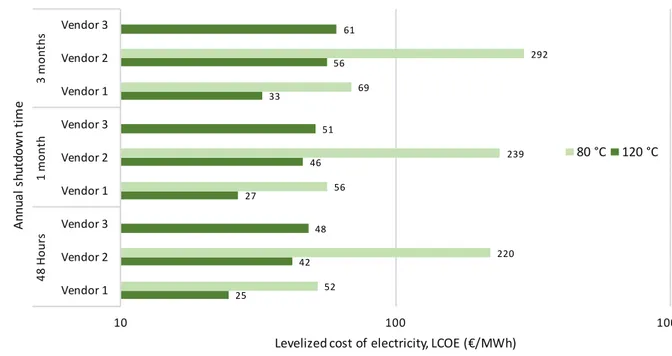
Figure 1 below shows the levelized cost of electricity in euro per MWh for three vendors, with 48 hours, 1 month, and 3 months of annual shutdown time. Across all vendors and temperature differentials, the LCOE ranges from 25 €/MWh to 292 €/MWh.
With shutdown times varying from 1 % (48 hour) to 25 % (3 months) per annum, the LCOE range is 25–33 €/MWh at the lowest cost option: Vendor 1 with 120 °C heat source. Vendor 1 also has the smallest cost range across all heat source temperatures and shutdown times: 25–69 €/MWh, whereas for Vendor 2 the range is 42–292 €/MWh. It should be noted that the optimal heat source temperature for Vendor 2 is stated to be 120 °C, whereas for Vendor 1 it is 90 °C. The efficiency of Vendor 2 at 80 °C is around 20 % of its efficiency at 120 °C. This demonstrates the importance of the combination of heat source temperature and working fluid selection. The LCOE range of Vendor 3 at 120 °C is 48–61 €/MWh, higher than the other vendors. This may relate to its maximum output, which is only 20 kWe, compared to 99 kWe and 150 kWe for the other two. Data was not available from Vendor 3 for an 80 °C heat source.
LFC =
TIC
1
(1+ r)
t t=1 T∑
÷
Q
LFC =
TIC
1− (1+ r)
−Tr
⎛
⎝⎜
⎞
⎠⎟
÷
Q = TIC
×
r
1− (1+ r)
−T÷
Q
LCOE = LFC + LVC =
TIC × r
1− (1+ r)
−T÷
Q
⎛
⎝⎜
⎞
⎠⎟
+ M
Q
3.2. Assumptions and variations in product data
Different vendors state different quantities for maintenance time per annum, installation costs, and product lifetime. Installation costs are particularly subjective and specific to each case, so for comparison the same percentage of device cost was used for vendor installation costs. Also, some vendors have a maximum heat source/sink pressure of 16 bar, whilst for others it is 9 bar. When connecting to a third-generation DH network, a pressure reduction device may therefore be necessary, e.g. a heat exchanger or substation, which may not be covered in the cost assumptions.
The technologies chosen are reliable, which is demonstrated by two vendors stating an annual maintenance time of just 48 hours. In the present study, shutdown times of 48 hours, 1 month, and 3 months are tested, to take account not only of the module maintenance schedule, but also the availability of non-fossil DH in the summer months.
The lifetime of the modules from the vendors is 20 years in two cases, and 15 years in another. The latter was determined in an interview to be a conservative estimate so all were considered to last 20 years for these calculations. 3.3. Calculating the levelized cost of electricity
Generically, LCOE is defined as the solution to the following equation described by Blumsack [8]:
(1) where, in year t, Ct represents the capital costs, Mt represents operational costs, Qt represents the annual energy
output, and r is the discount rate of capital. Solving equation 1 for LCOE gives:
(2)
If the annual output, Q, and the variable cost of production M, are the same each year, LCOE can be rewritten as the sum of the levelized fixed cost (LFC) and levelized variable cost (LVC):
(3) where LFC is the average payment to pay off the capital costs over T years and LVC is the average payment for per-unit operational costs. If the variable costs of production (variable operations and maintenance, fuel, and labor costs) are constant then LVC is the total variable cost per unit output, or M ÷ Q.
If the capital costs are paid in one lump sum – the total installed cost (TIC) – then LFC solves the equation: (4) where r is the discount rate of capital, and the life of the project is T years. This can be rewritten:
C
t+
M
t(1+ r)
t t=0 T∑
=
LCOE × Q
t(1+ r)
t t=0 T∑
=
LCOE
Q
t(1+ r)
t t=0 T∑
LCOE =
C
t+
M
t(1+ r)
t t=0 T∑
Q
t(1+ r)
t t=0 T∑
LCOE = LFC + LVC
TIC =
(1+ r)
LFC
t÷
Q
t=1 T∑
(5)and using convergence:
(6)
Combining equations 3 and 6 gives a simplified calculation of LCOE, for discount rate r and lifetime T:
(7)
3.4. LCOE calculation assumptions
The discount rate, r, is assumed to be 6 %, in line with other publications in this field, such as Nohlgren et al. [9]. The heat is assigned a zero cost, since it is highly dependent on the parameters of the DH network and beyond the scope of the present work. Exchange rates used are 1 USD = 0.92 EUR and 1 SEK = 0.10 EUR. Installation costs, and operation and maintenance costs used are those stated by the vendors. Electrical output is assumed to be 50 Hz (European electricity grids). The calculations do not take account of the pumping needs of the heat source or heat sink.
4. Results
Figure 1 below shows the levelized cost of electricity in euro per MWh for three vendors, with 48 hours, 1 month, and 3 months of annual shutdown time. Across all vendors and temperature differentials, the LCOE ranges from 25 €/MWh to 292 €/MWh.
With shutdown times varying from 1 % (48 hour) to 25 % (3 months) per annum, the LCOE range is 25–33 €/MWh at the lowest cost option: Vendor 1 with 120 °C heat source. Vendor 1 also has the smallest cost range across all heat source temperatures and shutdown times: 25–69 €/MWh, whereas for Vendor 2 the range is 42–292 €/MWh. It should be noted that the optimal heat source temperature for Vendor 2 is stated to be 120 °C, whereas for Vendor 1 it is 90 °C. The efficiency of Vendor 2 at 80 °C is around 20 % of its efficiency at 120 °C. This demonstrates the importance of the combination of heat source temperature and working fluid selection. The LCOE range of Vendor 3 at 120 °C is 48–61 €/MWh, higher than the other vendors. This may relate to its maximum output, which is only 20 kWe, compared to 99 kWe and 150 kWe for the other two. Data was not available from Vendor 3 for an 80 °C heat source.
LFC =
TIC
1
(1+ r)
t t=1 T∑
÷
Q
LFC =
TIC
1− (1+ r)
−Tr
⎛
⎝⎜
⎞
⎠⎟
÷
Q = TIC
×
r
1− (1+ r)
−T÷
Q
LCOE = LFC + LVC =
TIC × r
1− (1+ r)
−T÷
Q
⎛
⎝⎜
⎞
⎠⎟
+ M
Q
1726 Jay Hennessy et al. / Energy Procedia 142 (2017) 1721–1727
Fig. 1. LCOE from ORC with a heat sink of 20 °C and a heat source of 80 °C (light green) and 120 °C (dark green).
5. Discussion
The demonstrated sensitivity of the LCOE to heat source temperature has a clear significance in the context of DH, where temperatures lower than 90 °C and considerable temperature variability are both commonplace. The heat sink temperature will also vary depending on whether the DH return flow is used as a sink, or another source. The difference between heat source and heat sink temperatures is a primary factor affecting the power output.
During 2014–2016, the UK electricity market day-ahead spot price reached a maximum monthly average price of 68.5 €/MWh in November 2016. The yearly average in 2016 was 49.1 €/MWh. In the US state of New York, the average annual commercial price of electricity was 133.1 €/MWh in 2016. At an equivalent LCOE of 69 €/MWh for Vendor 1 at 80 °C with a 3-month shutdown period, DH-to-power use appears feasible under certain circumstances. These results do not account for the levelized cost of heat, nor varying heat source/sink temperatures, and further sensitivity analysis is needed for installation costs and spot prices.
6. Conclusions
From the studied vendor with the lowest LCOE range of 25–69 €/MWh, excluding the levelized cost of heat (LCOH), electricity generation from DH may be competitive against electricity spot market prices under certain circumstances, however a sensitivity analysis is necessary, as well as further calculations to determine how the LCOE would vary throughout the year with the constantly changing temperatures of a DH network and taking account of the LCOH. 25 42 48 27 46 51 33 56 61 52 220 56 239 69 292 10 100 1000 Vendor 1 Vendor 2 Vendor 3 Vendor 1 Vendor 2 Vendor 3 Vendor 1 Vendor 2 Vendor 3 48 H ou rs 1 m ont h 3 m ont hs Levelized cost of electricity, LCOE (€/MWh) Annua l s hut do w n tim e 80 °C 120 °C
Author name / Energy Procedia 00 (2017) 000–000 7 Acknowledgements
Special thanks to the participating vendors for their detailed data provided in confidence. The work has been carried out under the auspices of the Reesbe industrial post-graduate school, which is financed by the Knowledge Foundation (KK-stiftelsen), Sweden. The work was also part-financed by RISE Research Institutes of Sweden.
References
[1] International Energy Agency, “IEA Sankey Diagram,” 2014. [Online]. Available: https://www.iea.org/Sankey/#?c=World&s=Balance. [Accessed: 17-May-2017].
[2] S. Werner, “District heating and cooling in Sweden,” Energy, vol. 126, pp. 419–429, 2017.
[3] A. David, B. V. Mathiesen, H. Averfalk, S. Werner, and H. Lund, “Heat Roadmap Europe: Large-Scale Electric Heat Pumps in District Heating Systems,” Energies, vol. 10, no. 4, p. 578, 2017.
[4] B. F. Tchanche, G. Lambrinos, A. Frangoudakis, and G. Papadakis, “Low-grade heat conversion into power using organic Rankine cycles - A review of various applications,” Renew. Sustain. Energy Rev., vol. 15, no. 8, pp. 3963–3979, 2011.
[5] J. Karthäuser et al., “Distribuerad värmekraft i fjärrvärmenät,” 2016. Unpublished.
[6] Y. Wang, Q. Tang, M. Wang, and X. Feng, “Thermodynamic performance comparison between ORC and Kalina cycles for multi-stream waste heat recovery,” Energy Convers. Manag., vol. 143, pp. 482–492, 2017.
[7] C. E. Campos Rodríguez et al., “Exergetic and economic comparison of ORC and Kalina cycle for low temperature enhanced geothermal system in Brazil,” Appl. Therm. Eng., vol. 52, no. 1, pp. 109–119, 2013.
[8] S. Blumsack, “Project Decision Metrics: Levelized Cost of Energy (LCOE),” 2014. [Online]. Available: https://www.e-education.psu.edu/eme801/node/560. [Accessed: 24-May-2017].
Jay Hennessy et al. / Energy Procedia 142 (2017) 1721–1727 1727
Fig. 1. LCOE from ORC with a heat sink of 20 °C and a heat source of 80 °C (light green) and 120 °C (dark green).
5. Discussion
The demonstrated sensitivity of the LCOE to heat source temperature has a clear significance in the context of DH, where temperatures lower than 90 °C and considerable temperature variability are both commonplace. The heat sink temperature will also vary depending on whether the DH return flow is used as a sink, or another source. The difference between heat source and heat sink temperatures is a primary factor affecting the power output.
During 2014–2016, the UK electricity market day-ahead spot price reached a maximum monthly average price of 68.5 €/MWh in November 2016. The yearly average in 2016 was 49.1 €/MWh. In the US state of New York, the average annual commercial price of electricity was 133.1 €/MWh in 2016. At an equivalent LCOE of 69 €/MWh for Vendor 1 at 80 °C with a 3-month shutdown period, DH-to-power use appears feasible under certain circumstances. These results do not account for the levelized cost of heat, nor varying heat source/sink temperatures, and further sensitivity analysis is needed for installation costs and spot prices.
6. Conclusions
From the studied vendor with the lowest LCOE range of 25–69 €/MWh, excluding the levelized cost of heat (LCOH), electricity generation from DH may be competitive against electricity spot market prices under certain circumstances, however a sensitivity analysis is necessary, as well as further calculations to determine how the LCOE would vary throughout the year with the constantly changing temperatures of a DH network and taking account of the LCOH. 25 42 48 27 46 51 33 56 61 52 220 56 239 69 292 10 100 1000 Vendor 1 Vendor 2 Vendor 3 Vendor 1 Vendor 2 Vendor 3 Vendor 1 Vendor 2 Vendor 3 48 H ou rs 1 m ont h 3 m ont hs Levelized cost of electricity, LCOE (€/MWh) Annua l s hut do w n tim e 80 °C 120 °C
Author name / Energy Procedia 00 (2017) 000–000 7 Acknowledgements
Special thanks to the participating vendors for their detailed data provided in confidence. The work has been carried out under the auspices of the Reesbe industrial post-graduate school, which is financed by the Knowledge Foundation (KK-stiftelsen), Sweden. The work was also part-financed by RISE Research Institutes of Sweden.
References
[1] International Energy Agency, “IEA Sankey Diagram,” 2014. [Online]. Available: https://www.iea.org/Sankey/#?c=World&s=Balance. [Accessed: 17-May-2017].
[2] S. Werner, “District heating and cooling in Sweden,” Energy, vol. 126, pp. 419–429, 2017.
[3] A. David, B. V. Mathiesen, H. Averfalk, S. Werner, and H. Lund, “Heat Roadmap Europe: Large-Scale Electric Heat Pumps in District Heating Systems,” Energies, vol. 10, no. 4, p. 578, 2017.
[4] B. F. Tchanche, G. Lambrinos, A. Frangoudakis, and G. Papadakis, “Low-grade heat conversion into power using organic Rankine cycles - A review of various applications,” Renew. Sustain. Energy Rev., vol. 15, no. 8, pp. 3963–3979, 2011.
[5] J. Karthäuser et al., “Distribuerad värmekraft i fjärrvärmenät,” 2016. Unpublished.
[6] Y. Wang, Q. Tang, M. Wang, and X. Feng, “Thermodynamic performance comparison between ORC and Kalina cycles for multi-stream waste heat recovery,” Energy Convers. Manag., vol. 143, pp. 482–492, 2017.
[7] C. E. Campos Rodríguez et al., “Exergetic and economic comparison of ORC and Kalina cycle for low temperature enhanced geothermal system in Brazil,” Appl. Therm. Eng., vol. 52, no. 1, pp. 109–119, 2013.
[8] S. Blumsack, “Project Decision Metrics: Levelized Cost of Energy (LCOE),” 2014. [Online]. Available: https://www.e-education.psu.edu/eme801/node/560. [Accessed: 24-May-2017].