Using Supervised Learning and Data Fusion to Detect Network Attacks

VÄSTERÅS, SWEDEN

Bachelor Thesis in Computer Science – 15.0 credits

USING SUPERVISED LEARNING AND DATA

FUSION TO DETECT NETWORK ATTACKS

Jesper Hautsalo

jho14002@student.mdh.se

Examiner:

Sasikumar Punnekkat

Mälardalen University, Västerås, Sweden

Supervisor: Miguel León Ortiz

Mälardalen University, Västerås, Sweden

Abstract

Network attacks remain a constant threat to organizations around the globe. Intrusion detection systems provide a vital piece of the protection needed in order to fend off these attacks. Machine learning has become a popular method for developing new anomaly-based intrusion detection systems, and in recent years, deep learning has followed suit. Additionally, data fusion is often applied to intrusion detection systems in research, most often in the form of feature reduction, which can improve the accuracy and training times of classifiers. Another less common form of data fusion is decision fusion, where the outputs of multiple classifiers are fused into a more reliable result. Recent research has produced some contradictory results regarding the efficiency of traditional machine learning algorithms compared to deep learning algorithms. This study aims to investigate this problem and provide some clarity about the relative performance of a selection of classifier algorithms, namely artificial neural network, long short-term memory and random forest. Furthermore, two feature selection methods, namely correlation coefficient method and principal component analysis, as well as one decision fusion method in D-S evidence theory were tested. The majority of the feature selection methods fail to increase the accuracy of the implemented models, although the accuracy is not drastically reduced. Among the individual classifiers, random forest shows the best performance, obtaining an accuracy of 87,87%. Fusing the results with D-S evidence theory further improves this result, obtaining an accuracy of 88,56%, and proves particularly useful for reducing the number of false positives.

Table of Contents

1.

Introduction ... 5

2.

Background ... 6

3.

Related Work ... 12

4.

Problem Formulation ... 14

5.

Method ... 15

6.

Ethical and Societal Considerations ... 16

7.

Implementation and experiment ... 17

8.

Results ... 19

9.

Discussion ... 23

10.

Conclusions ... 24

11.

Future Work ... 25

Table index

Table 1. The results of the CCM evaluation test ... 19

Table 2. The results of the PCA evaluation test ... 19

Table 3. ANN test results highlighting accuracy in validation and testing, as well as FNR and FPR in testing ... 20

Table 4. LSTM test results highlighting accuracy in validation and testing, as well as FNR and FPR in testing ... 20

Table 5. RF test results highlighting accuracy in validation and testing, as well as FNR and FPR in testing ... 21

Table 6. Test results showing accuracy, FNR and FPR of the selected individual classifiers and the DST classifier ... 21

Table 7. Comparison of the best classifiers for each algorithm ... 22

Figure index

Figure 1. A simplistic example of an Artificial neural network structure... 9

Figure 2. Confusion matrix of all the best classifiers ... 22

Equation index

Equation 1. Pearson correlation coefficient ... 9

Equation 2. Rectified linear unit ... 10

Equation 3. Hyperbolic tangent ... 10

Equation 4. Sigmoid function ... 10

1. Introduction

With the rapid and seemingly never-ending growth of the Internet, network security faces an ever-expanding list of challenges, all while it becomes more and more important. Network attacks are a major concern for virtually any organization, as they can compromise services or confidential information. As many sectors become increasingly reliant on the internet, network attacks grow more complex and the types and variations of attacks more numerous. In order to maintain proper operations, organizations must be able to defend themselves against such network attacks.

Intrusion Detection Systems (IDS) provide a vital part of the protection an organization needs to protect themselves. Briefly put, the purpose of an IDS is to detect a network attack as early as possible, which would then further allow another service, a network administrator, or another agent to take an appropriate action. IDS have been widely used for decades, but just like the attacks they aim to detect, IDS in general have evolved much since their inception. There are two broad categories of IDS: signature-based and anomaly-based. A signature-based IDS monitors network packets and searches them for signatures of known network attack types. Anomaly-based IDS learns the general behaviour of normal network traffic and raises an alarm when significant deviations from this normal behaviour is detected. Both categories have their strengths and weaknesses, which are explained later in this report, but in general, signature-based detection is more limited because of its inability to detect unknown types of attacks. As such, most of the recent research in this area have focused on researching and developing new and better anomaly-based intrusion detection systems.

Machine learning (ML) has been extensively used in research to develop new IDS for some time now. ML has proven an excellent tool for anomaly detection in general, and more recently, deep learning (DL) has also made significant advances in the field. In this study I investigated several supervised machine learning algorithms, as well as data fusion algorithms, in the context of anomaly-based IDS. This report covers a selection of related work where supervised learning and data fusion is used to construct robust IDS models. Many studies compare the results of their experiments to other studies to put their results into perspective. However, this can be challenging with IDS, as the performance of an IDS depends heavily on a number of factors that are not always consistent between studies. For this reason, I conducted an experiment where I compared the performance of several supervised learning classifier algorithms. I also analyzed the performance of multiple data fusion techniques and algorithms in conjunction with the aforementioned classifier algorithms.

The rest of this report is structured as follows: Section 2 gives an overview of intrusion detection, the used evaluation metrics for testing, a selection of relevant datasets, an overview of data fusion and the used algorithms in this study. Section 3 provides an overview of the related work reviewed for this study. Section 4 contains the problem formulation and gives the motivation of the study. Section 5 details the methods used in the study. Section 6 discussed some ethical considerations related to AI. Section 7 details the implementation and the experiment, section 8 presents the results, which are further discussed in section 9. Finally, section 10 concludes the report.

2. Background

This section will provide a thorough explanation of IDS and its importance for cybersecurity. The different categories of IDS will be explained, and I also provide an overview of the recent developments in the area. The evaluation metrics typically used for IDS are then defined. A selection of the most popular datasets are also discussed, after which I motivate my choice of dataset for this study. Lastly, data fusion is briefly overviewed, after which I discuss it in more detail in the context of IDS.

2.1 Intrusion detection

IDSs have been around for a long time. The basic function of an IDS is quite simple: analyze network packets with the goal of labelling them as normal (benign) or abnormal (attack) [1]. By labelling the network packets as such, an IDS can enable other defense mechanisms, or a network administrator, to deploy appropriate countermeasures to either prevent the attack or minimize the damage caused by it. There are two basic categories of IDS, signature-based and anomaly-signature-based, both with their advantages and disadvantages.

Signature-based IDS is the more traditional category. Simply put, a signature-based IDS operates by analyzing packets for signatures of known network attack types and labels the packets accordingly [1]. The main advantages of signature-based IDS are that they are computationally cheap and quite effective at detecting known attack types. The largest, and quite obvious, disadvantage of signature-based IDSs is their complete inability to detect unknown network attack types, as they rely on a database of known attack types in order to perform the classification. Whilst signature-based IDS are an effective first-line of defence against network attacks thanks to their low computational cost, they are not sufficient as the only detection mechanism, as day-zero attacks become more and more common. Anomaly-based detection could be described as the opposite of signature-based detection. Where signature-based IDS learn the signature of different attack types, anomaly-based IDS learn the normal behaviour of the network, and labels packets that deviate from this normal behaviour as attacks [1, 2]. This enables anomaly-based IDSs to overcome the glaring weakness of signature-based IDSs, as they have the ability to detect previously unknown types of network attacks. However, compared to signature-based IDSs, anomaly-based detection is generally more computationally expensive. As they both have their strengths and weaknesses, the two categories are often used in tandem to provide an overall good IDS.

As for classification, it too can be done in one of two ways: binary classification or multi-class classification. Binary classification labels the data packets as either normal or attack, making no distinction between different types of attacks [3]. Multi-class classification labels the packets as either normal or as a specific type of attack, for example DDoS. Much like the different categories of IDS, both of these classification types have advantages and disadvantages. In a real environment, multi-class classification would be more useful, as you need to know which type of attack the network is being subjected to in order to deploy appropriate countermeasures. On the other hand, in order the detect a previously unknown type of attack, binary classification needs to be performed. Again, much like the IDS categories, these two can be used in tandem to strengthen the robustness of the IDS. For example, a classifier that performs binary classification can be used at first, and if a packet is labelled as an attack, it can be sent to a multi-class classifier to identify the attack type.

Nowadays, most research focuses on anomaly-based detection, as its application is less limited than signature-based detection. Some time ago, machine learning made significant breakthroughs in the field of anomaly-signature-based detection, and more recently deep learning followed suit. As such, the aim of this study is to investigate different supervised machine learning methods in the context of anomaly-based intrusion detection.

2.2 Evaluation metrics

Throughout this report, several evaluation metrics will be used to describe some aspect of the performance of an IDS. The definitions of all these metrics are presented in this subsection. These definitions are based on [2], but they are consistent with all reviewed literature in this report.

Positives and negatives

A positive refers to a record that was labelled as an attack by the classifier, while a negative refers to a record that was labelled as normal activity. As such, a true positive (TP) is a correctly classified attack and a false positive (FP) is normal activity incorrectly classified as an attack. Conversely, a true negative (TN) is normal activity correctly classified as such, and a false negative (FN) is an attack incorrectly classified as normal activity.

Accuracy

Accuracy, represented as a percentage, denotes the proportion of correctly classified compared to the total amount of records. As such, it is defined as following:

𝐴𝑐𝑐𝑢𝑟𝑎𝑐𝑦 = 𝑇𝑁 + 𝑇𝑃

𝑇𝑁 + 𝑇𝑃 + 𝐹𝑁 + 𝐹𝑃

Precision

Precsion, also represented as a percentage, is a measurement of the number of true positives compared to the total amount of positives, and is defined as:

𝑃𝑟𝑒𝑐𝑖𝑠𝑖𝑜𝑛 = 𝑇𝑃 𝑇𝑃 + 𝐹𝑃

False-positive rate and false-negative rate

False-positive rate (FPR) and false-negative rate (FNR) are useful measurements to analyze the error rate of the classifier. FPR represents the percentage of normal traffic classified as attacks compared to the total number of normal traffic records. FNR represents the percentage of attacks classified as normal traffic compared to the total number of attack records.

𝐹𝑃𝑅 = 𝐹𝑃 𝐹𝑃 + 𝑇𝑁

𝐹𝑁𝑅 = 𝐹𝑁

𝐹𝑁 + 𝑇𝑃

Recall

Recall denotes the percentage of detected attacks compared to the total number of attack records, and as such can be used to describe a classifiers chance to detect a network attack.

𝑅𝑒𝑐𝑎𝑙𝑙 = 𝑇𝑃 𝑇𝑃 + 𝐹𝑁

Specificity

Specificity is the opposite of recall, and as such is a measurement of the percentage of correctly classified normal records compared to the total number of normal records

𝑆𝑝𝑒𝑐𝑖𝑓𝑖𝑐𝑖𝑡𝑦 = 𝑇𝑁 𝑇𝑁 + 𝐹𝑃

2.3 Datasets

The vast majority of experiments in the area of IDS are conducted using one or more preexisting datasets. These datasets have their own strengths and weaknesses, which will be discussed in this section. What they all have in common is that they are comprised of a collection of preproccessed network data, called features. Some datasets use real captured network activity, while others use simulated activity. Every connection in the dataset is labelled as either normal activity, or as some type of network attack. Some datasets also have a specified training and testing sub-dataset. The features and labels can thus be used to train supervised machine learning algorithms to detect network attacks. The rest of this section will discuss a selection of datasets that have been very popular in prior research. Lastly, I will motivate my choice of dataset for the experiment conducted in this study.

Quite possibly the most popular dataset, the KDD99 dataset was generated from the DARPA 1998 dataset [1]. It has 41 features and was created in a simulated military environment in 1998. Besides normal traffic, KDD99 features four types of network attacks: Denial of Service (DoS), Probe, User-to-Root (U2R) and Remote-to-Local (R2L). The distribution of these attack types in the training set is heavily imbalanced, however, with almost 20% of the data consisting of normal traffic and almost another 80% consisting of DoS attacks [4]. One the main benefits of the KDD99 dataset is that is has been widely used in prior research, enabling direct comparisons for new research. However, because of its age, arguments can be made that the dataset fails to properly represent the nature of modern network attacks [1].

In 2009, tavallaee et al. proposed a new dataset, NSL-KDD. This dataset consisted of records extracted from the KDD99 dataset but was created to solve several issues with the KDD99 dataset, such as the number of redundant

records used. Since then, the NSL-KDD has also been widely used as a benchmark dataset [3]. However, some of the inherent weaknesses of the KDD99 dataset remains, such as its notable age.

In more recent year, the UNSW-NB15 dataset has seen much use in research. N. Moustafa and J. Slay proposed this dataset in 2015 and argued that it better represented the modern nature of network attacks [5]. In [6], N. Moustafa and J. Slay also demonstrate that the UNSW-NB15 dataset is more complex than the KDD99 dataset. It consists of a mixture of real normal traffic and simulated attacks. It features nine different types of network attacks, compared to the four in KDD99 and NSL-KDD. UNSW-NB15 has 45 features and a separate training and testing set. Considering the increased number of attack types, as well as the fact that it is a much newer dataset, it can be argued that UNSW-NB15 is a more realistic benchmark dataset. For this reason, it was my dataset of choice for this study.

2.4 Data fusion

Data fusion as a concept stems from the 80’s, where it was first introduced in the military field [1]. Since then, multiple definitions for the term have been proposed. In general, data fusion can be quite simply described as the combination of data from multiple sources into a singular output. Data fusion is universally performed in order to improve the accuracy or reliability of the output. In the field of network intrusion detection, the goal of data fusion would be to improve any of the following: accuracy, precision, false-positive rate and false-negative rate. Prior research indicates that data fusion for NIDS can be especially effective for reducing the negative and false-positive rates [7,8].

According to Li et al. [1], data fusion can be applied in three different levels: (i) data level, (ii) feature level and (iii) decision level.

i. Data level fusion combines multiple raw data into a set of data that is expected to be more informative. In the case of network intrusion detection, this raw data would refer to various network data. Because of the widespread use of preexisting datasets by research in the field of NIDS, data fusion is rarely investigated, as the raw network data has already been extracted and refined into the datasets in question. ii. Feature level fusion can be used to select a subset of data features deemed to be most important. In NIDS,

feature fusion is often referred to as feature reduction, and many studies [3,9,10,11] use feature reduction to improve the performance of their proposed models. Many different algorithms can be used to perform feature reduction, and some studies [9] even manually select a subset of features. Feature reduction is generally useful for reducing redundant features which only serve to worsen the results of the used model. Feature fusion also serves to reduce computation time, as fewer features need to be considered by the model.

iii. Decision level fusion, or simply decision fusion, fuses the decisions of multiple detectors. This is done to improve the accuracy or general reliability of the system, and much like feature reduction, it can be done in multiple ways. A system utilising decision fusion can take advantage of the ability to apply multiple different detectors, which could be used to cover weaknesses of individual detectors. Unlike feature reduction, computation time is a major challenge with decision fusion, and should be considered accordingly.

In this study data level fusion will not be applied as a preexisting dataset will be used. I will therefor also not discuss it any further. Feature reduction on the other hand has been proven to be almost universally beneficent [12]. In this study, I investigated multiple feature reduction methods, based on the reviewed literature in section 3. Evaluating different feature reduction methods can however be challenging, as the results of a certain method is entirely dependent on the dataset it is applied to and the classification algorithm used. It is thus difficult to make general claims about the efficiency of individual feature reduction methods. As stated, many studies use some sort of feature reduction method, but fewer studies compare multiple feature reduction methods. Additionally, the amount of research investigating decision fusion in the context of IDS is currently limited.

2.5 Algorithms

This section will provide a rundown of all the algorithms used in this work. The aim is to provide readers that are unfamiliar with the topics a reasonable grasp of the work conducted in association with this report. The first subsection covers the algorithms used for feature reduction, the second subsection covers the algorithms used for classification, and the last subsection covers D-S Evidence Theory, which was used for decision fusion.

2.5.1 Feature reduction

This subsection provides an overview of the algorithms used for feature reduction in this study, namely correlation coefficient method and principal component analysis.

Correlation coefficient method

Correlation coefficient method (CCM) measures the correlation between two variables [10]. This means that two variables with a very high correlation are close to linearly associated, whereas two variables with a low correlation are not. There are multiple variants of CMM, and in this report, as in [10], I used the Pearson correlation coefficient, calculated as:

Equation 1. Pearson correlation coefficient

𝜌𝑋,𝑌 =

𝑐𝑜𝑣(𝑋, 𝑌) 𝜎𝑋𝜎𝑌

In this formula, cov is the covariance and 𝜎 is the standard deviation. The idea is then that one variable in a pair of variables with a high correlation can be eliminated, as they will be close to linearly associated, and might thus have a very similar effect on the output.

Principal Component Analysis

The goal of principal component analysis (PCA) is to extract a number of features from a set that are the most representative of the whole set [1]. In doing so, the dimensionality of the set can be reduced whilst still maintaining the majority of the information of the original set. PCA extracts new variables, called principal components, from the original set. The first component has the largest variance, and us thus the most representative of the entire set. All components after the first are calculated the same way, with the restriction that they are orthogonal to the components before them.

2.5.2 Classification

This subsection covers the algorithms used for classification in this study, namely artificial neural network, long short-term memory, and random forest.

Artificial neural network

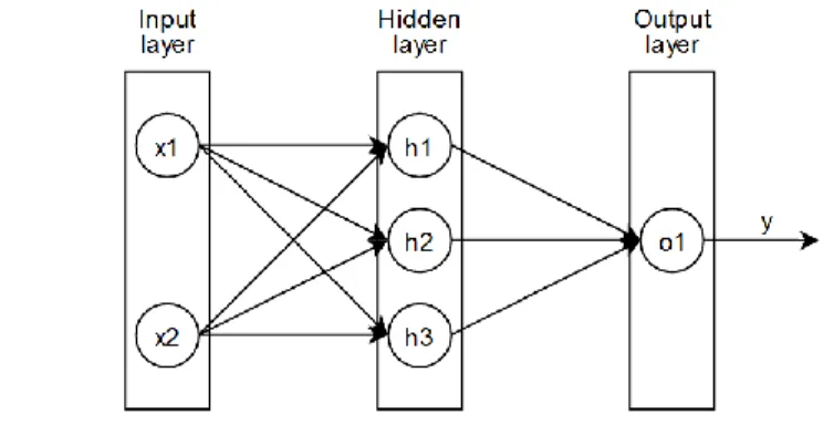
An artificial neural network (ANN) consists of many units, often called neurons [1]. Each neuron has an output, several inputs, and an associated weight for each input. Neurons are categorized into layers, namely input layers, hidden layers, and output layers. All neurons in a layer are connected to every neuron in its neighbouring layer. Figure 1 visualizes a very simplistic ANN.

Figure 1. A simplistic example of an Artificial neural network structure

In figure 1, 𝑥1 and 𝑥2 are two input neurons. As can be seen, they are both connected to all neurons in the hidden

layer, ℎ1−3. All neurons in the hidden layer are also connected to the neuron in the output layer, 𝑜1. Each

connection has an associated weight, which is randomized upon initialization. The neurons in the hidden layer and output layer also have activation functions. An activation function determines the output of a neuron and can thus

be used to produce more desirable outputs. In this study, I use the Rectified Linear Unit (ReLU), hyperbolic tangent (tanh) and Sigmoid activation functions. What they all have in common is that all inputs are first multiplied by their associated weight, and then summed together. If we refer to this sum as 𝑥, these activation functions can then be defined as follows:

Equation 2. Rectified linear unit

𝑅𝑒𝐿𝑈(𝑥) = {0,_𝑥, 𝑓𝑜𝑟 𝑥 ≤ 0_{𝑓𝑜𝑟 𝑥 > 0} (𝑅𝑒𝐿𝑈)

Equation 3. Hyperbolic tangent

𝑡𝑎𝑛ℎ(𝑥) =(𝑒

𝑥_{− 𝑒}−𝑥₎

(𝑒𝑥_{+ 𝑒}−𝑥₎ (𝑡𝑎𝑛ℎ)

Equation 4. Sigmoid function

𝜎(𝑥) = 1

1 + 𝑒−𝑥 (𝑆𝑖𝑔𝑚𝑜𝑖𝑑)

ReLU simply converts any negative values to zero, tanh squishes values to a continuous interval between -1 and 1, and Sigmoid, similarly to tanh, squishes values into a continuous interval between 0 and 1.

ANNs are then trained by feeding extensive amounts of labelled data through them. Take for example a simple ANN used binary network attack classification. The network would need as many input neurons as there are features in the network data. The hidden layer(s) can have any number of neurons, and the output layer would only need one neuron. In this case, the Sigmoid activation function, which limits any value to a number between zero and one, could be used for the output layer. That way, an output closer to zero would indicate a “normal” classification, and an output closer to one would indicate an “attack” classification. During training, the output of the network and the label of the input data are then used to define an error term, which describes how far off target the network was for every record. This error is then fed backwards through the network and is used to update all weights to better account for the error. This way the ANN can “learn” from its mistakes and improve its performance over multiple epochs of training.

Recurrent neural network and long short-term memory

A recurrent neural network (RNN) is very similar to an ANN, the difference being that an RNN can propagate past information in the hidden layer to the hidden layer at the current time [9]. It accomplishes this using feedback loops in the hidden layer where information can persist for a time. In this way, an RNN can consider both current as well as past information when performing classification. RNNs face a major weakness in the so-called vanishing gradient problem. In basic RNNs, less recent information will have a smaller significance than more recent information held in the internal feedback loop. This can result in “old” information becoming insignificant, which in turn will hinder the network from learning from long-distance dependencies. Essentially, the RNN has a short-term memory. The solution this problem is long short-short-term memory (LSTM). LSTMs solve this problem by incorporating certain gates. These gates help the network decide which data is more important, and which data is less important. By doing this, the less important data can be safely forgotten, which in turn allows the more important data to be held in memory for longer, solving the vanishing gradient problem.

Random forest

Random forest (RF) is an ensemble algorithm, meaning that it makes use of multiple decision trees to present a final classifier [13]. The basic idea of RF is that a large group of trees working together will outperform a single tree. During training, a number of random trees, which attempt to correctly classify the data, will be created, after which the best performing tree will be chosen as the classifier. Compared to the neural networks described above, RF is computationally inexpensive, which makes it an interesting candidate for IDS.

D-S evidence theory

D-S evidence theory, short for Dempster-Shafer evidence theory (DST), is a method for dealing with uncertainty [1]. The basic idea of DST is that probabilities are estimated via intervals, rather than single values. These intervals represent the lower (belief) and upper (plausibility) bounds of probability, meaning that some room for uncertainty is made. Belief can then be assigned to each hypothesis for each unit, or classifier in the case of IDS. The beliefs of each classifier can then be combined using Dempsters rule of combination. To define this rule, we assume that there are two classifiers with a certain belief in support of a hypothesis [7]. The beliefs will be referred to as 𝑚1

and 𝑚2. Additionally, B is the set of hypotheses for classifier 1, and C is the set of hypotheses for classifier 2. The

combined belief of these classifiers, 𝑚1,2, can then be defined as follows:

Equation 5. Dempsters rule of combination

𝑚1,2(𝐴) =

∑𝐵∩𝐶=𝐴𝑚1(𝐵)𝑚2(𝐶)

∑𝐵∩𝐶=0𝑚1(𝐵)𝑚2(𝐶)

Using Dempsters rule of combination, the results of multiple classifiers can be combined to improve the results. Multiple studies have shown that DST can be useful for lowering the FPR of IDS [7].

3. Related Work

There is a vast amount of research on anomaly-based IDS. Much of the most recent research focuses on deep learning, but some recent research on more traditional machine learning has also been done. This section gives an overview of the reviewed literature. The literature is roughly divided into research investigating different classification algorithms and research investigating decision fusion for IDS.

Yin et al. [3] uses a Recurrent Neural Network (RNN) for network anomaly detection. The NSL-KDD dataset is used for benchmarking, and the authors claim that their proposed model performs better than many other machine learning methods, such as ANN, RF, support vector machine (SVM), etc. The model is tested with many different hidden nodes and learning rates. The best configuration, as tested on the KDDTest+ dataset, obtained an 83.28% accuracy in binary classification and 81.29% accuracy in multi-class classification. Both results were better than their review literature. In the multi-class classification test, the highest FPR was 2.16%, given by the Probe intrusion type. The R2L and U2R intrusion types only obtained a detection rate of 24.69% and 11.50% respectively. These two intrusion types did however have significantly fewer training samples than other intrusion types.

Roy et al. [9] proposes a Bi-Directional Long Short-Term Memory Recurrent Neural Network (BLSTM RNN) to detect network attacks common in Internet of Things (IoT) environments. The model is tested in binary classification, using a manually reduced version of the UNSW-NB15 dataset. The model obtains an accuracy of 95.71% in binary classification. Notably, the model also obtained zero false positives in testing, resulting in a precision of 100% and a very low recall of 96%.

Cheng et al. [14] proposes a Multi-Scale LSTM (MS-LSTM) for anomaly detection in Border Gateway Protocol (BGP) traffic. The authors note that the randomness of internet traffic can cause issues for many anomaly-based detection systems, and they propose LSTM as a remedy for this. The authors find that LSTM is efficient for reducing the false-alarm rate. The study also investigates the effect of different time scales on LSTM and concludes that a properly selected time scale can increase the accuracy of the model significantly. In the best case, the model obtains a 99.5% accuracy in binary classification. The experiment does not use a publicly available dataset. Kshirsagar and Kumar [15] proposed a model that combined information gain and correlation to reduce the features of the CICDDoS2019 dataset. A j48 classifier is then used to detect different DDoS attacks and achieves good results.

Alamiedy et al [11]. performed a study where Grey Wolf Optimization was used to reduce the features of the NSL-KDD dataset into an optimal subset. SVM was then used to perform multi-class classification. The proposed model obtained an average accuracy of 87.59%. It can be noted that this model encountered a similar weakness as the one in [3], where the detection rate of the R2L and U2R attack types were significantly lower than the other types. In a very recent study, Xuan et al. [10] claims that overly complicated and computationaly costly algorithms are not necessary in developing a robust detection system. They propose a model using the Random Forest (RF) method and claim that it is the current best classification technique. Additionally, they investigate different feature reduction methods, such as correlation coefficient method, information gain method and principal component analysis. The model performs binary classification and testing is done on a reduced version of the UNSW-NB15 dataset, as the authors argue that it provides the most realistic results.

Concerning decision fusion, some research has been made, although not as extensively as the amount of existing research around IDS. Recently, Nguyen et al. [12] performed a study where they proposed a model that fuses the decisions from multiple IDSs using different classification algorithms. Features are reduced using a Chaotic Butterfly Optimization Algorithm (CBOA), and the decisions of CNN, LSTM and GRU classifiers are fused to create the final classification result. Results for every separate classifier, as well as the fused classifier, are presented with and without the CBOA feature selection. The study thus provides a good insight into the effect of both feature selection and decision fusion, but it has a few shortcomings. The fused classification is binary, and the authors do not make it clear exactly how the data is fused. Furthermore, it can be observed that some of the classification algorithms obtain a worse result with feature selection compared to without, which might indicate a non-optimal feature selection method.

To summarize, we can clearly see that extensive research already exists in the area of anomaly-based intrusion detection. However, some of the reviewed literature makes contradictory claims about the performance of various detection methods. Several studies, such as [14] and [3] argues that more traditional machine learning methods are unable to achieve results matching those produced by these studies. Additionally, many studies [14, 16 ,3] claim that deep learning methods in general outperform traditional ML methods. Despite this, the study in [10] produces good results using Random Forest, a traditional ML method. This might be an indicator of the significance of effective feature reduction, the used dataset, and the difficulty of comparing binary to multi-class classification.

4. Problem Formulation

As illustrated in the previous section, there is already a lot of research in the field of IDS. Most research aims at either developing completely new, or new versions of existing classification methods. Some contradictory claims can be observed between various research, however, raising uncertainty about the results of said research. Most notably, some research claims that deep learning is superior to traditional machine learning methods, whilst some other research claims that simpler algorithms, such as RF, can still compete with more advanced methods. For this reason, I wanted to investigate both deep learning methods as well as more traditional machine learning methods, in order to compare the performance between the two.

Most experiments in the reviewed literature include some sort of feature reduction method, although these are typically not discussed in great detail. Some research that investigates different decision fusion methods in the context of IDS has also been done, although this has not been as extensively researched as classification methods. For this reason, I wanted to evaluate a selection of feature reduction methods, as well as a decision fusion method. Making relative comparisons between different studies is difficult, as the performance of a model can be impacted by the choice of dataset, feature reduction method or other variables. As such, I believe that performing a single study where multiple methods are evaluated on equal grounds can provide a more reliable comparison. Based on the reviewed literature, the main contributions of this work are as follows:

• Provide further insight into the relative performance of a selection of classifiers based on supervised learning algorithms, feature reduction methods and decision fusion methods.

• Provide insight into the performance effect of different feature reduction and decision fusion methods.

4.1 Research questions

The main questions I aim to answer can then be defined as follows:

• Which supervised learning algorithm is the most effective at detecting network attacks? • How can data fusion be applied to improve the results further?

4.2 Limitations

This study will be limited to two different feature reduction algorithms, three classifier algorithms and one decision fusion algorithm. It will also be limited to using only the UNSW-NB15 dataset, more specifically the pre-defined training and testing sets, and the tests will only be performing binary classification. My choice of algorithms is motivated in section 5.

5. Method

To answer my proposed questions, and to provide the proposed contribution, I performed a literature study and an experiment. The aim of the literature study was to increase my own knowledge of the area in general, as well as to compile a selection of related work that I could relate my own work to. In the experiment I implemented and evaluated several IDSs. For these IDSs, I implemented several feature reduction algorithms, classifier algorithms and finally a decision fusion algorithm. The general order of operations during this experiment was thus as follows: • Implement a classifier algorithm. The classifier was tested and evaluated without any feature reduction. • Once the classifier was implemented and achieved reasonable results, I implemented and applied a feature

reduction algorithm. The IDS was then tested and evaluated with the feature reduction algorithm. • The first two steps were then repeated for every classification algorithm and every feature reduction

algorithm.

• After this, every classifier algorithm and their respectively best feature reduction algorithms were selected as the candidates for the decision fusion testing. Here, the chosen decision fusion algorithm was implemented, tested, and evaluated.

In total, I implemented and tested two feature reduction algorithms, three classifier algorithms and one decision fusion algorithms. The feature reduction algorithms were Principal Component Analysis (PCA), and Correlation coefficient method (CCM). The classifier algorithms were Long Short-Term Memory (LSTM), Artificial Neural Network (ANN) and Random Forest (RF). Finally, the decision fusion method was D-S Evidence Theory. All variations of the IDSs were implemented in Python, and the ANN and LSTM classifiers were implemented using the Keras library, while the RF classifier was implemented using the scikit-learn library. After every classifier was tested and evaluated, I analyzed the results. Here I made notes on the performance of the best individual classifiers, as well as the fused classifier, and compared it to the related work.

6. Ethical and Societal Considerations

The rapid advance of AI has contributed to solving many problems around the world. However, this rapid advance has also raised a number ethical concerns regarding AI. Some issues are more ambiguous in nature, such as the usage of AI in healthcare to diagnose patients [17]. Other issues stem from unethical use of AI, such as the Chinese governments use of facial recognition to distinguish certain minorities from the rest of the population [18]. When developing AI, great care should be taken to consider the intented and otherwise possible usage of said AI. As far as research in the field of network security goes, I consider this study to be overwhelmingly positive regarding any ethical dilemmas. Further research on intrusion detection systems can contribute to the cybersecurity of many organizations, which I consider to be a good thing.

As this study did not in any way include any personal or otherwise sensitive information, ethical issues related to such aspects were not applicable.

7. Implementation and experiment

7.1 Data preprocessing

Before using the dataset, some preprocessing needed to be done. As stated earlier, the pre-existing training and testing sets of the UNSW-NB15 dataset was used. The training set has 175341 records, and the testing set has 82332. Firstly, non-numerical values need to be converted into numerical values. In the training and testing sets, this is done on the attack categories (attack_cat), protocols (proto), services (service), and states (state). The conversion is done by gathering all existing values of each type into an array, after which each non-numerical value takes on the numerical index of said value. When this is done, the attack categories (attack_cat) and binary labels (label) are split off from the rest of the dataset, which creates a set of features, a set of labels and a set of binary labels. Lastly, all subsets of the training set will be split into training and validation sets, with a respective 7:3 ratio. This effectively means that 70% of the original training set will be used to train the models, while 30% of it will be used to evaluate and revise the models in pursuit of the best performance. It was noticed that simply dividing the data as explained resulted in a validation set consisting entirely of attack records, as the number of false positves for all initial tests were zero. The entire dataset was thus shuffled randomly to address this issue. The end result was a set of training data, validation data, testing data, as well as respective labels for all of the sets.

7.2 Feature reduction

Pandas offers a built-in function to calculate the correlation between variables in a dataframe. This function, corr(), was used with the “pearson” argument to calculate the pearson coefficients of the dataframe. This way, an arbitrary coefficient threshold can be set, and values surpassing this threshold can be filtered out. A smaller experiment was conducted using a RF classifier to find the best coefficient value. This value was then used for all other experiments for all classifiers. The result of this initial experiment is presented in section 8.

The PCA feature selection was implemented using scikit-learn. With scikit-learn, an arbitrary number of desired features can be selected through the “n_components” argument, after which the training set can be used to select the best features according to the provided number. Here, I conducted a similar small experiment with RF, where different numbers of features were tested in order to find the optimal number. After this experiment, the chosen features were extracted from the training, validation and testing sets for all other experiments.

7.3 Classification

The ANN and LSTM models were implemented using the Keras deep learning library. The preprocessed and reduced dataframes were first converted into Numpy arrays to be compatible with Keras. The data is then normalized, before being used as input for the models. Multiple iterations of the ANN and LSTM models were implemented and tested, which will be further presented in section 8. All experiments used a 20% dropout after each hidden layer, meaning that 20% of the input values of that layer, chosen at random, were set to zero and thus are effectively dropped. This can help reduce overfitting [19]. For the LSTM layers, the tanh activation function was used, while the ReLu function was used for the ANN hidden layers. Finally, the output layers of both the ANN and LSTM models used the Sigmoid activation function, as a binary output was desired. All versions of the ANN and LSTM models were training over 200 epochs.

The RF model was implemented using the scikit-learn library. As in [10], information gain was used to split the features, by setting the “criterion” argument to “entropy”. Multiple numbers of trees were tested for the RF model, as presented in section 8.

7.4 Decision fusion

Before passing the output of the individual classifiers to a fusion classifier, the outputs need some cleaning. This is because Keras and scikit-learn prints the outputs of the models in different formats, and as such they need to be homogenised before further use. Keras outputs non-binary values between zero and one in an array format, meaning every value is enclosed by brackets, whereas scikit-learn simply outputs binary values. I used a separate program to remove the brackets from each Keras output value, after which I round the values to either zero or one. After this, the new values are saved in a csv-file, where each row contains one value. This is done for both the cleaned Keras outputs as well as the scikit-learn outputs, and it makes it easy to load the values into new dataframes before being used for data fusion.

In the decision fusion, depending on the output of the classifiers, their respective TPRs or TNRs, as recorded during testing, was used as the belief for that classfier. If a classifier had labelled a record as an attack, the TPR

was used as that classifiers belief that the record was an attack, and as such the belief for that record being normal was 1-TPR. The same logic was used for classifiers when they labelled records as normal, but here TNR was used instead of TPR. Dempsters rule of combination was then applied to combine the beliefs of the selected classifiers for each record in the testing set, which produced the final resulting classifications.

8. Results

This section details the results from the various experiments performed in the study. It is divided into subsections covering each classifier, used with and without the selected feature reduction methods. The results of the decision fusion are then presented, and finally, the best performing classifiers from each category are compared to each other and the fused DST classifier.

8.1 Feature selection evaluation

This subsection presents the results from the feature selection evaluation experiment. The RF classifier with 40 trees was used to evaluate multiple coefficients for CCM, as well as multiple numbers of features for PCA. The accuracies presented are from the validation set and can be seen in tables 1 and 2 below.

Correlation coefficient method

Ten different coefficients were tested for the CCM feature selection. Table 1 presents the values of these coefficients, the number of extracted features and the validation accuracy based on a RF classifier using the extracted features. Surprisingly, most of the tests yielded worse results than RF produced without any feature selection, although the variations in the results are fairly small. The only test that achieved improved results was CCM with a coefficient value of 1, which resulted in only one feature to be removed. As the goal of the experiment was to maximize accuracy, this coefficient value was thus used for further tests with CCM.

Table 1. The results of the CCM evaluation test

FS

Features

Validation Accuracy (%)

None 42 95,73 CCM-1 41 95,86 CCM-0,9 30 95,35 CCM-0,8 29 95,28 CCM-0,7 25 95,26 CCM-0,6 22 95,26 CCM-0,5 17 94,61 CCM-0,4 16 94,53 CCM-0,3 16 94,48 CCM-0,2 13 94,55 CCM-0,1 7 93,51

Principal component analysis

Seven different numbers of features were tested for the PCA feature selection. Much like with CCM, PCA yielded worse results than RF without feature selection, this time without exception. The variations in the results are also slightly larger here compared to CCM, but they show a steady decline that roughly correlates to the number of features used. As PCA with 35 features gave the best results out of the tested versions, it was used for further tests with PCA.

Table 2. The results of the PCA evaluation test

FS

Validation Accuracy (%)

None 95,73 PCA-35 95,34 PCA-30 95,24 PCA-25 94,92 PCA-20 94,56 PCA-15 94,08 PCA-10 92,11 PCA-5 91,30

8.2 Artificial neural network

With the optimal FS methods decided, the classification algorithms could now be tested. Table 3 presents the performance of the various ANN configurations after 200 epochs of training. For each FS method, three different configurations of the ANN were tested; (i) one hidden layer with 150 neurons (units), (ii) two hidden layers with 75 neurons each, and (iii) three hidden layers with 50 neurons each. The first column, FS, shows which feature selection method was used for that test. The second column shows how many hidden layers were used in the configuration, and the third column shows how many units were used in each layer.

Table 3. ANN test results highlighting accuracy in validation and testing, as well as FNR and FPR in testing

FS

Layers Units Validation

acc (%)

Testing

acc (%)

Testing

FNR (%)

Testing

FPR (%)

None 1 150 94,80 85,61 2,30 29,18 2 75 94,93 86,21 1,48 28,86 3 50 94,85 85,56 2,36 29,24 CCM 1 150 94,69 87,79 3,08 23,38 2 75 94,79 85,67 1,23 30,37 3 50 94,76 85,51 2,02 29,76 PCA 1 150 94,97 87,00 2,56 25,78 2 75 94,95 86,65 3,06 25,94 3 50 94,92 87,01 1,24 27,37

As can be seen, the best performing classifier was the ANN with one layer, 150 units and CCM feature selection, obtaining a testing accuracy of 87,79%. It can be noticed that the models with better accuracy are generally the ones with lower FPR, as FNR seems to be much less important. However, the recorded validation accuracy indicates that the ANN with two layers, 75 units and no FS was the best one, and as such, that model was used for the decision fusion.

8.2 Long short-term memory

Table 4 presents the results of the various LSTM configurations that were tested. The tested LSTM configurations were identical to the ANN ones, where three different configurations per FS method were used.

Table 4. LSTM test results highlighting accuracy in validation and testing, as well as FNR and FPR in testing

FS

Layers Units Validation

acc (%)

Testing

acc (%)

Testing

FNR (%)

Testing

FPR (%)

None 1 150 94,99 86,04 3,11 27,25 2 75 95,13 85,97 2,73 27.86 3 50 95.07 86,27 2,76 27,15 CCM 1 150 94,96 86,77 3,87 24,68 2 75 95,14 86,28 2,82 27,05 3 50 95,01 87,04 3,39 24,68 PCA 1 150 95,08 86,78 3,40 25,25 2 75 95,30 85,01 3,76 28,72 3 50 95,11 84,62 4,51 28,69

Here, the LSTM model with three layers, 50 units and CCM FS yielded the best accuracy, at 87,04%, in testing. Similar to the tested ANN models, reducing the FPR seems to be the most important factor in improving the accuracy of the LSTM models, as the FPR is generally quite high. Validation indicated that the model with two layers and PCA FS was the best one, and thus it was selected to be used in the decision fusion.

8.3 Random forest

Four numbers of trees were tested for each FS method for the RF classifier, namely 10, 40, 100 and 200 trees. The results of these tests are presented in table 5.

Table 5. RF test results highlighting accuracy in validation and testing, as well as FNR and FPR in testing

FS

Trees

Validation

acc (%)

Testing

acc (%)

Testing

FNR (%)

Testing

FPR (%)

None 10 95,65 87,67 2,69 23,33 40 95,77 87,25 1,77 26,16 100 95,89 87,18 1,52 26,64 200 95,93 87,11 1,50 26,82 CCM 10 95,43 87,87 2,42 24,00 40 95,78 87,30 1,71 26,14 100 95,80 87,16 1,56 26,63 200 95,86 87,05 1,55 26,89 PCA 10 94,93 85,84 3,72 26,92 40 95,39 85,69 2,11 29,25 100 95,31 85,51 1,90 29,89 200 95,46 85,33 1,87 30,34

The best model was the one with ten trees and CCM feature selection, achieving 87,87% accuracy in testing. In fact, it can be observed that the accuracy drops as the number of trees increases in all tests. It can also be observed that the opposite is true for the validation accuracy for almost all tests, which indicated that the validation set did not represent the testing set well. Based on the validation accuracy, the model with 200 trees and no FS was the best one, and so it was selected for the decision fusion.

8.4 D-S evidence theory

For the DST decision fusion, the outputs of the best classifier, based on the validation accuracy, from each category above was picked for the fusion test. Thus, the ANN with two layers and no FS, LSTM with two layers and PCA FS, and RF with 40 trees and no FS was used. Their respective TPR and TNR were then used as the appropriate beliefs, depending on wether they labelled a record as normal or attack. The result of the fusion is presented in table 6 below.

Table 6. Test results showing accuracy, FNR and FPR of the selected individual classifiers and the DST classifier

Classifier

Testing

acc (%)

Testing

FNR (%)

Testing

FPR (%)

ANN 86,21 1,48 28,86 LSTM 85,01 3,76 28,72 RF 87,11 1,50 26,82 DST 88,56 2,41 22,48

Here it can be observed that DST manages to slightly improve the results of the best single classifier. As expected based on the reviewed literature, the FPR of the DST classifier is drastically reduced compared to the single classifiers, although the same cannot necessarily be said about the FNR. However, as observed in the previous tests, reducing the FPR seems to be the most important factor in increasing the accuracy of a model, as FPR is generally much higher than FNR.

8.5 Final results

This subsection compares the performances of all the best individual classifiers as well as the DST classifier. Figure 2 below shows the confusion matrices of the best ANN, LSTM and RF classifiers, as well as the DST classifier.

Figure 2. Confusion matrix of all the best classifiers

From figure 2 we can see that RF has a notably lower FNR compared to ANN and LSTM. The DST classifier has a very similar FNR to the RF classifier, but also has a notably lower FPR. Table 7 illustrates these results further.

Table 7. Comparison of the best classifiers for each algorithm

Classifier Accuracy (%) FNR (%)

FPR (%)

Precision (%) Recall (%)

Specificity (%)

ANN 87,79 3,08 23,38 83,54 96,91 76,61

LSTM 87,04 3,39 24,68 82,74 96,60 75,31

RF 87,87 2,42 24,00 83,27 97,57 75,99

DST 88,56 2,41 22,48 84,16 97,58 77,51

Here it can clearly be seen that DST outperforms all the other classifers in every regard, even when using the outputs of the sub-optimal individual classifiers. The most notable difference is once again the comparably low FPR, which directly contributes to a notably higher specificity.

9. Discussion

Many of the experiments conducted yielded surprising results. Most notably, the feature reduction methods employed were ineffective in regards to increasing the accuracy, almost without exception, which was contrary to my expectation. Compared to the reviewed literature, [10] used very similar methods when using both CCM and PCA for feature reduction and achieved good results. One notable difference is that they used a far larger dataset, which might have an impact on the performance of said methods. In [15], the authors intersect the results of several FS methods, including CCM, to create their final set of features. Combining multiple methods like this might be more reliable than using a single method. It can also be noted from table 1 that the difference in validation accuracy is less than half a percent between the test where no CCM was applied and the test where CCM with a coefficient threshold of 0.6 was applied. This is interesting as the number of features extracted with a coefficient of 0.6 was 22, almost half of the original 42. This means that a small amount of accuracy could be sacrificed in the favor of faster training and classification times, which in some scenarios might be a valid alternative. Furthermore, it should also be noted that the best ANN, LSTM and RF classifiers based on the testing accuracy all used CCM feature selection. This might indicate that the validation set did not represent the testing set well, and that perhaps other coefficients for CCM could indeed have yielded better results in testing.

As for classification, changing the configurations of the different classifiers had a very minor impact on the performance, as a small degree random variance should be expected between tests. All three algorithms showed similar performance, with RF slightly outperforming ANN and LSTM. ANN and LSTM are somewhat famous for their high FPR, and it can be observed that many of the testet RF models beats them in that regard, although the best ANN had a lower FPR compared to the best RF model. It should however be noted that both the ANN and LSTM models were trained over 200 epochs, which is arguably a low number. Further testing with more configurations and longer training times for ANN and LSTM would thus be interesting, as that might yield better results. Even so, one should not disregard RF simply because of its fast training and classification speed. Even using 200 trees, RF was still many times faster than ANN, which was in turn much faster than LSTM in terms of training. In general, the models in this study did not match many of the models in the related work in terms of accuracy. In addition to the explanation above, this could also be the result of the simple classifiers used in this study. For example, in this study I implemented a basic LSTM model, whereas [9] implemented a bi-directional LSTM and [14] implemented a multi-scale LSTM.

D-S evidence theory proved useful for further improving the results of invidivual classifiers. Most notably, the FPR was reduced by over 3% compared to the best individual classifier used in the fusion (table 6), and almost 1% compared to the best individual classifier with the lowest FPR (table 7). It is thus clear that decision fusion is a powerful tool for increasing the performance of an IDS.

10. Conclusions

The aim of this study was to compare a selection of classifier algorithms used in instrusion detection systems, as well as to investigate how data fusion could impact the performance of said algorithms. This was done by investigating several classifiers, feature selection methods and a feature fusion method in the context of intrusion detection systems. The feature selection methods tested were correlation coefficient method and principal component analysis. The classifier algorithms were artificial neural network, long short-term memory and random forest. The decision fusion method was D-S evidence theory. All tests were conducted using the UNSW-NB15 dataset.

In terms of accuracy, the feature selection methods yielded disappointing results, and further research is required into how they can be improved. Overall, the loss of accuracy was small, however, and it could be argued that trading a small amount of accuracy for a vastly reduced set of features can be worth it. As for the classifier algorithms, random forest performed surprisingly well, considering its exponentially shorter required training time compared to both ANN and LSTM. Of all the tested individual classifiers, random forest obtained the highest accuracy of 87,87%. The different configurations of each classifier did not seem to have a large impact on the result. D-S evidence theory improved the results by a small amount and proved useful for reducing the number of false positives of the classifiers. The fused DST classifier outperformed the aforementioned RF classifier, obtataining an accuracy of 88,56%. It can thus be concluded that decision fusion is very useful for further improving the performance of individual classifiers.

11. Future Work

This study could be vastly expanded upon in the future. As with any study that focuses on comparisons between different algorithms or methods, it would be beneficial to maximize the number of algortihms compared. In this case, more feature reduction methods, classifier algorithms and data fusion methods could be explored to expand the scope of the study. Not only would it be relevant to compare more individual classifiers, but in doing so more classifiers could also be used in the decision fusion, which might yield interesting results. By expanding the scope of the study, the relevance of the results produced would be increased, as the study would be more comprehensive and less cherry-picked.

Furthermore, more advanced versions of the classifiers used in this study could also be explored. As noted in section 9, few of the individual classifiers included in the experiment of this study matched the performance of similar classifiers in the related work. This could be at least partially explained by the fact that I implemented basic versions of most classifiers for this study, whereas much of the related work used more advanced versions of the same classifiers. Additionally, the results of the feature selection did not match the expectations set by the related work, and as such, this needs to be investigated further.

References

[1-1] G. Li, Z. Yan, Y. Fu, H. Chen, "Data Fusion for Network Intrusion Detection: A Review", Security and

Communication Networks, vol. 2018, pp 1-16, May 2018, doi: 10.1155/2018/8210614

[2] S. Hajj, R. El Sibai, J. Bou Abdo, J. Demerjian, A. Makhoul, C. Guyeux, “Anomaly-based intrusion detection systems: The requirements, methods, measurements, and datasets”, Transactions of Emerging

Telecommunications Technologies, 2021, doi: 10.1002/ett.4240.

[3] C. Yin, Y. Zhu, J. Fei, X. He, “A Deep Learning Approach for Intrusion Detection Using Recurrent Neural Networks”, in IEEE Access, vol. 5, pp. 21954-21961, 2017, doi: 10.1109/ACCESS.2017.2762418.

[4] Bagui, S., Li, K. Resampling imbalanced data for network intrusion detection datasets. Journal of Big Data, vol. 8, article 6, Dec 2021, doi: 10.1186/s40537-020-00390-x.

[5] N. Moustafa, J. Slay, “UNSW-NB15: a comprehensive data set for network intrusion detection systems (UNSW-NB15 network data set)”, Military communications and information systems conference (MilCIS), article 7348942, 2015, doi: 10.1109/MilCIS.2015.7348942.

[6] N. Moustafa, J. Slay, “The evaluation of Network Anomaly Detection Systems: Statistical analysis of the UNSW-NB15 dataset and the comparisons with the KDD99 data set”, Information Security Journal, vol 25, issue 1-3, pp 18-31, 2016, doi: 10.1080/19393555.2015.1125974.

[7] Y. Zhang, S. Huang, S. Guo,J. Zhu, ”Multi-sensor Data Fusion for Cyber Security Situation Awareness”,

Procedia Environmental Sciences, vol. 10, pp. 1029-1034, 2011, doi: 10.1016/j.proenv.2011.09.165.

[8] J. Tian, W. Zhao, R. Du, Z Zhang, ”A New Data Fusion Model of Intrusion Detection-IDSFP”, in 3rd

International Symposium on Parallel and Distributed Processing and Applications, Nanjing, China, 2005, pp

371-382. [Online]. Available: https://link.springer.com/chapter/10.1007%2F11576235_40, accessed on 2021-04-18. [9] B. Roy, H. Cheung, “A Deep Learning Approach for Intrusion Detection in Internet of Things using Bi-Directional Long Short-Term Memory Recurrent Neural Network”, 2018 28th _{International Telecommunication}

Networks and Applications Conference (ITNAC), Sydney, Australia, 2018, pp .1-6, doi: 10.1109/ATNAC.2018.8615294.

[10] C.D. Xuan, H. Thanh, N.T. Lam, “Optimization of network traffic anomaly detection using machine learning”

International Journal of Electrical and Computer Engineering, vol. 11, issue 3, June 2021, pp 2360-2370, doi:

10.11591/ijece.v11i3.pp2360-2370.

[11] T.A. Alamiedy, M. Anbar, Z.N.M. Alqattan, Q.M. Alzubi, “Anomaly-based intrusion detection system using muti-objective grey wolf optimization algorithm”, Journal of Ambient Intelligence and Humanized Computing, vol. 11, issue 9, Sep. 2020, pp. 3735-3756, doi: 0.1007/s12652-019-01569-8.

[12] P. T. Nguyen, V. Dang, K. D. Vo, P. T. Phan, M. Elhoseny et al., "Deep learning based optimal multimodal fusion framework for intrusion detection systems for healthcare data," Computers, Materials & Continua, vol. 66, no.3, 2021, pp. 2555–2571, doi: 10.32604/cmc.2021.012941.

[13] H. Tyagi, R. Kumar, “Attack and Anomaly Detection in IoT Networks Using Supervised Machine Learning Approaches”, Revue d’Intelligence Artificielle, vol. 35, issue 1, Feb 2021, pp 11-21, doi: 10.18280/ria.350102. [14] M. Cheng, Q. Xu, J. Lv, W. Liu, Q. Li, J. Wang, ”MS-LSTM: a Multi-Scale LSTM Model for BGP Anomaly Detection”, 2016 IEEE 24th International Conference on Network Protocols (ICNP), Singapore, 2016, pp. 1-6, doi: 10.1109/ICNP.2016.7785326.

[15] D. Kshirsagar, S. Kumar, “A feature reduction based reflected and exploited DDoS attacks detection system”,

[16] Y. Wu, D. Wei, J. Feng. "Network Attacks Detection Methods Based on Deep Learning Techniques: A Survey", Security and Communication Networks, vol. 2020, pp. 1-17, Aug. 2020, doi: 10.1155/2020/8872923. [17] K. Murphy, E. Di Ruggiero, R. Upshur, D. J. Willison, N. Malhotra, J. Ce Cai, N. Malhotra, V. Lui, J. Gibson, “Artificial intelligence for good health: a scoping review of the ethics literature”, BCM Medical Ethics, vol. 22, article 14, 2021, doi: 10.1186/s12910-021-00577-8.

[18] R. Van Noorden, “The ethical questions that haunt facial-recognition research”, Nature, vol. 587, pp 354-358, 2020, doi: 10.1038/d41586-020-03187-3

[19] Keras, “Dropout layer”, 2021. [Online]. Available: https://keras.io/api/layers/regularization_layers/dropout/, retrieved: 2021-05-26.