UPTEC F13018
Examensarbete 30 hp
Juni 2013
Solving the Vehicle Routing
Problem
using Search-based Methods and PDDL
Gösta Agerberg
Teknisk- naturvetenskaplig fakultet UTH-enheten Besöksadress: Ångströmlaboratoriet Lägerhyddsvägen 1 Hus 4, Plan 0 Postadress: Box 536 751 21 Uppsala Telefon: 018 – 471 30 03 Telefax: 018 – 471 30 00 Hemsida: http://www.teknat.uu.se/student
Solving the Vehicle Routing Problem using
Search-based Methods and PDDL
Gösta Agerberg
In this project the optimization of transport planning has been studied. The approach was that smaller transport companies do not have the capability to fully optimize their transports. Their transport optimization is performed at a company level, meaning that the end result might be optimal for their company, but that potential for further optimization exists.
The idea was to build a collaboration of transport companies, and then to optimize the transports globally within the collaboration. The intent was for the collaboration to perform the same driving assignments but at a lower cost, by using fewer vehicles and drivers, or travel shorter distance, or both combined. This should be achieved by planning the assignments in a smarter way, for example using a company's empty return journey to perform an assignment for another company.
Due to the complexity of these types of problems, called Vehicle Routing Problem (VRP), shown to be NP-complete, search methods are often used. In this project the method of choice was a PDDL-based planner called LPG-td. It uses enforced hill-climbing together with a best-first search to find feasible solutions. The method was tested for scaling, performance versus another method and against time, as well as together with a real-life based problem.
The results showed that LPG-td might not be a suitable candidate to solve the problem considered in this project. The solutions found for the collaboration were worse than for the sum of individual solutions, and used more computational time. Since the solution for the collaboration at most should be equal to the sum of individual solutions, in theory, this meant that the planner failed.
ISSN: 1401-5757, UPTEC F13018 Examinator: Tomas Nyberg Ämnesgranskare: Pierre Flener Handledare: Carl Svärd
Popular scientific abstract in Swedish
Sammanfattning
I detta projekt har optimeringen av transportplanering undersökts. Ansatsen var att mindre åkerier inte har möjlighet att till fullo optimera sina transporter. De-ras optimeringar är gjorda baserade på åkeriets egna körningar, vilket betyder att resultatet kan vara optimalt, men att möjligheter för optimering fortfarande kan finnas. Det kan exempelvis röra sig om lastbilar som kör tomma åt ett håll, eller tidsfönster som gör att ett företag måste använda en extra lastbil för en enda körning.
Idén var att en grupp åkerier skulle gå ihop i en kollaboration för att kunna optimera sin transportplanering globalt inom den. Kollaborationen skulle på så sätt utföra precis samma transportuppdrag men till en lägre kostnad, genom att använda färre antal lastbilar och förare, eller köra kortare distans, eller båda sam-tidigt. Detta skulle åstadkommas genom att planera körningarna smartare, och för exempel utnyttja att företag A kör sin tomma lastbil hem efter ett uppdrag, till att lastbilen kör samma rutt men med ett uppdrag för företag B.
Komplexiteten på problem som detta, på engelska kallade Vehicle Routing Problems, har visats vara NP-kompletta. Detta har inneburit att sökmetoder har blivit populära för att lösa dessa problem, och det är också en typ av sökmetod som använts i detta projekt. Metoden som används grundar sig på ett standardise-rat planeringsspråk (eng.: Planning Domain Definition Language) och en planera-re som heter LPG-td. LPG-td använder två metoder, hill-climbing och best-first, för att hitta godkända lösningar. I projektet testades LPG-td:s prestanda, skal-ningsförmåga samt slutgiltligen mot ett verklighetsbaserat problem.
Resultaten visade att LPG-td inte kan ses som en potentiell kandidat för att lö-sa de typer av transportproblem som är betraktade i detta projekt. Lösningen för kollaborationen var sämre än summan av de individuella lösningarna — och an-vände mer beräkningstid. Teoretiskt ska kollaborationens lösning minst kunna vara lika bra som summan av de individuella, vilket betyder att LPG-td miss-lyckades med att hitta de lösningar som hittades för de individuella åkerierna.
1 Introduction 7 1.1 Background . . . 7 1.2 Long-term Goals . . . 8 1.3 Project Goals . . . 9 1.4 Outline . . . 9 2 Problem Description 11 2.1 Different Kinds of Vehicle Routing Problems . . . 11
2.2 What Has Been Studied Before . . . 11
2.2.1 Branch and Bound . . . 12
2.2.2 Ant Colony Optimization . . . 12
2.2.3 Genetic Algorithms . . . 12
2.2.4 Hybrid . . . 13
2.2.5 Financial Aspects . . . 13
2.3 The Vehicle Routing Problem in this Project . . . 13
2.4 Restrictions and Interpretation . . . 14
2.5 Constraints . . . 15
2.6 Objective Function . . . 15
3 Search-Based Problem Solving 17 3.1 Search Algorithms . . . 17 3.2 PDDL . . . 17 3.3 Versions of PDDL . . . 18 3.4 LPG-td . . . 18 3.4.1 PDDL Features . . . 19 3.4.2 Planning . . . 20 3.4.3 LPG-td Accomplishments . . . 24 4 Implementation 25 4.1 Domain File . . . 25 4.1.1 Types . . . 25 4.1.2 Predicates . . . 25 4.1.3 Functions . . . 26 4
CONTENTS 5 4.1.4 Actions . . . 26 4.2 Problem File . . . 27 5 Evaluation 29 5.1 Definitions . . . 29 5.2 Different Planners . . . 30 5.3 LPG-td Scaling . . . 34 5.4 LPG-td Performance . . . 39 5.5 LPG-td Relative Improvement . . . 42
5.6 Case Study Problem . . . 43
6 Conclusions 49 7 Discussion 51 7.1 Transport and Solving Problems . . . 51
7.1.1 Choice of Planner . . . 51
7.1.2 Understanding How the Planner Works Versus Usability . 52 7.1.3 Heuristics . . . 52
7.1.4 Soft Constraints . . . 52
7.1.5 Adaptivity of PDDL . . . 52
7.2 Financial Aspects . . . 53
7.2.1 Is There Anyone Interested in a Service Like This? . . . 53
7.2.2 Sharing Profits and Resources Between Participants . . . . 53
7.2.3 How to Approach Companies in Best Fashion . . . 54
7.2.4 Assumption of No Rivalry Among Participants . . . 54
7.2.5 Financial Regulations and Laws Against Collaborations . . 54
8 Acknowledgements 57
Bibliography 59
A Matlab Code 61
1
Introduction
1.1
Background
A problem within the transport business is the relatively small profit margin at about 3,5-4 % [10]. This is especially troublesome for small transport companies which of course do not have the same financial stability to withstand periods of bad economy, or perhaps the financial possibilities to grow as a company. The number of small transport companies in Sweden is very high, with companies having 1-5 Heavy Duty Vehicles (HDV) making up for 84 % [11] of the total
Swedish fleet as seen in Figure 1.1. Because a lot of these small transport com-panies are customers to Scania, and their existence and need of new HDVs is in Scania’s interest, Scania decided to investigate the possibilities to increase their profit margin.
One possibility, and the option treated in this thesis, would be to increase the transport companies’ profitability by optimizing their transport planning. A problem for the small transport companies is that with a small number of HDVs, the local transport planning optimization in terms of routing might be difficult and yield a sub-optimal solution with low fill-rates. For example they might have to go empty on the way back from a driving assignment, thus effectively reduc-ing the fill-rate by half. If they could find an assignment for the way back, or at least in the near proximity of the return journey, they could increase the revenue while maintaining a cost that is almost the same (more fuel will be needed, but the static costs for the HDV and the driver are the same).
Figure 1.1:Swedish fleet sizes 2011 [11]
1.2
Long-term Goals
The vision Scania has is to support small transport companies with a service that provides them with the possibility to share driving assignments with other sim-ilar companies. This would mean that they could trade driving assignments, by either buying, selling or switching, trying to optimize their fill-rate and cutting their costs. The sharing of assignments should increase the fill-rate, thus making it possible to transport the same amount of goods with fewer HDVs or less driven distance. This would decrease some of the costs for the companies, for example making it possible to perhaps manage with one less HDV and driver, while the revenue stays constant.
1.3 Project Goals 9
The reasons for Scania to help reduce the number of HDVs might not be easy to see, but with an increased profit margin for the transport companies, Scania could also increase their profit margin, thus produce fewer HDVs but make more money on each of them. This would also allow Scania to expand their horizon into becoming a service provider which could be a new area where profits could be made. Finally, one could also provide this service with the requirement that customers have to pay, either a monthly or a one-time sum.
The pure economical aspect is not the only one though, as more optimized routing should lead to reduced pollution, and a better environment. Since fewer drivers would be needed, this opens up labour for other jobs.
1.3
Project Goals
The main goals of this project are to investigate whether a collaboration between transport companies can be accomplished, and whether the transport optimiza-tion could be done using a PDDL-based planner.
This is done mainly by solving the vehicle routing problem associated with transport companies, first company by company, and for the fictitious collabora-tion. The desired result would show a reduced cost that is sufficient to encourage and motivate transport companies into consideration of collaborating.
To do this as close to real-life as possible, data from real transport companies is extracted and used as a base to create a problem instance to validate the model. Regarding the financial side of the problem, the profits would have to be shared, using a system that makes both the driving assignment seller and buyer content. This is a very interesting and hard problem that lies beyond the scope of this thesis.
1.4
Outline
The rest of this thesis is structured as follows: first, a problem description is given, together with an explanation of the restrictions and interpretations that were used (Chapter 2). Next comes the method used in this master thesis, along with a description of LPG-td, the planner used in this work (Chapter 3). Then follows a chapter briefly describing how the implementation was done (Chapter 4), and the results (Chapter 5). Conclusions of the thesis are then given (Chapter 6) before a chapter with a discussion is presented as the final piece (Chapter 7).
2
Problem Description
2.1
Different Kinds of Vehicle Routing Problems
There are several different types of vehicle routing problems (VRPs), and they have been studied extensively. The standard VRP consists of a number of vehi-cles and locations together with a number of driving assignments. The rules are set that each location has to be visited exactly once by a single vehicle, and the vehicle starts and finishes at a depot.
On top of the standard version, there are a lot of different types. They range from problems including Time Windows (VRPTW)1, to problems dealing with Capacity constraints (CVRP) 2, and those where goods can be Simultaneously Picked up and Delivered (VRPSPD)3(the depot is not used as goods central any more). There are many more as well, including several combinations of the above mentioned types.
2.2
What Has Been Studied Before
The area of solving different variants of VRP is a field which has been studied intensively. Since the problem has been shown [20] to be NP-complete 4, the use of heuristics and approximate solutions plays a big part in finding solutions.
1http://neo.lcc.uma.es/radi-aeb/WebVRP/index.html?/Problem_ Descriptions/VRPTWDesc.htmlaccessed on 2013-05-27 2http://neo.lcc.uma.es/radi-aeb/WebVRP/index.html?/Problem_ Descriptions/CVRPDesc.htmlaccessed on 2013-05-27 3http://neo.lcc.uma.es/radi-aeb/WebVRP/index.html?/Problem_ Descriptions/VRPPDDesc.htmlaccessed on 2013-05-27 4http://www.mathsisfun.com/sets/np-complete.htmlaccessed on 2013-06-17 11
Different search algorithms have been used, among the most common ones are probabilistic algorithms, simulated annealing, local search methods or, a combi-nation of different methods (hybrid)5.
2.2.1
Branch and Bound
One of the historically first papers to deal with VRPSPD is [13], which studies the distribution of books from a library in USA. The solving method was to first clus-ter the assignments according to geographical proximity, then to split the prob-lem into two parts. The first part became a Travelling Salesman Probprob-lem (TSP) and the second part dealt with satisfying the constraints derived from the loading coupled to the capacity constraints. The complete solution was then derived by solving the TSP, and then checking if the solution satisfied the constraints in part two. If the solution found for the TSP did not satisfy the constraints, a penalty was given to the route and then another iteration of TSP was performed.
2.2.2
Ant Colony Optimization
Another method to solve VRP’s is by applying a probabilistic method like for example Ant Colonization Optimization (ACO). In [14], a couple of different real-life VRP’s with time windows, VRPTW’s, are solved using ants and pheromones. The basic idea is to send out ants in the search graph and use heuristics, called pheromones, to make them choose the best route. Each ant represents a solution to either the full problem or to a section of it. The heuristics are based on both a priori and posteriori knowledge, and indicate the probability that an ant will choose a specific route. The probability depends on both the estimated desirabil-ity to choose that route, and the number of ants that have chosen that specific route previously.
2.2.3
Genetic Algorithms
In [18], the possibility to use genetic algorithms is displayed. A genetic algorithm works by finding a solution, and then trying to improve that solution by either
breeding or mutating. Breeding means that two solutions, the parents, are
com-bined to make a third one, the child. The child consists of parts from its parents, chosen by a routine. Mutating means that a solution is partially randomly trans-formed, creating an offspring with some new features. After either one, or both, the new solutions are evaluated and by some selection routine and probability, new parents are chosen.
5http://neo.lcc.uma.es/radi-aeb/WebVRP/index.html?/Problem_
2.3 The Vehicle Routing Problem in this Project 13
2.2.4
Hybrid
A combined approach was used in [2], where Simulated Annealing (SA) and Large Neighbourhood Search (LNS) are combined into a hybrid solver. This al-gorithm works by first using SA to decrease the number of routes, and then LNS to decrease the total travel cost. SA works by permuting a solution into another one, and accepting the new solution as the current one if certain conditions are fulfilled. The new solution is accepted as the current if it:
• is better than the previous best,
• is worse than the previous best, but the randomly generated variable p is greater than a parameter that decreases with the temperature,
• together with all other new solutions is worse than the previous best, and none have satisfied the condition above, one solution is randomly chosen. The parameter that decides whether or not a worse solution is accepted is the key for SA. It is often described as e−∆t , where t is the temperature and ∆ is chosen
to either make it easy or hard for worse solutions to pass. The temperature de-creases for each iteration SA performs, thus inferior solutions will have less and less probability to be accepted as the number of iterations increases. The best solution is stored and after a maximum time limit is reached, it is returned.
To reduce the total travel cost LNS was used. Bent and van Hentenryck de-scribes the use with
’The main idea behind LNS is to iteratively remove subsets of cus-tomers (gradually increasing the number of cuscus-tomers to remove at a time) from the best known solution and explore their feasible reinser-tion points in a systematic fashion’ [2, p. 881].
2.2.5
Financial Aspects
The financial aspects were considered in the beginning of this project, and though they are not covered in this thesis, they raise questions about the solutions of the problem of sharing the profits within the collaboration. Moreover, in [3] the order when approaching customers was discussed, together with mentioning the Shap-ley value. Different methods to share the profit have been studied extensively, for example in [1], [6], and [19].
2.3
The Vehicle Routing Problem in this Project
The problem in this thesis is a classical vehicle routing problem, combined with a couple of constraints that make it hard to solve. The main goal is to perform a number of driving assignments, delivering a number ofparcels, from a set of
customers to another set of customers. This means that the parcels are picked up during driving assignments and then carried by an HDV to a given location.
The driving assignments are also specified by time windows that set the earliest possible pick-up time as well as the latest possible delivery time. At the end of the day, the HDV should return back to its origin.
What makes this an interesting, and even more difficult, problem is that an HDV could perform assignments simultaneously, or instead of returning empty it could perform an assignment that has its delivery location close to where the HDVs origin is — thus decreasing the total cost. Another way to further decrease the cost — and consequently make the entire fleet more effective, is to use fewer HDVs and optimize the routing.
A difference to many of the problems studied, is that a parcel is specified to go between two pre-defined locations, thus it is not considered as an interchange-able material (for example sand) that could be thought of simply by its weight or volume. This makes the problem studied in this thesis to be a combination of CVRP, VRPTW, and VRPSPD.
The problem might not be solved using one of the algorithms found in the literary study, due to the complex constraints — especially the possibility of per-forming multiple driving assignments at once. With some modification it could be possible, but this has not been further studied in this thesis.
2.4
Restrictions and Interpretation
To make the problem solvable within the time given, certain restrictions are nec-essary. It is also necessary to state how the problem was interpreted, which leads to the solution design.
To begin with, the planning problem is assumed to be of a size and complex-ity that makes an analytical optimization intractable. This means that a search method of some kind is needed, and that the global optima might not be possible to find.
The restrictions are constructed to simplify the problem, and start with the fact that drivers are not considered. This means that driving constraints such as laws about resting, licenses for different HDVs etc. are neglected. Moreover, all HDVs are considered to be of the same type and size, which in turn also leads to the simplification that any assignment is considered possible to perform with any HDV. Again, this simplifies the problem and reduces the amount of different objects.
Although assignments are simplified to be stackable with all other assign-ments, they have individual time windows and weights.
2.5 Constraints 15
2.5
Constraints
HDVs
Capacity Constraint— The constraint that is concerning the HDVs in the prob-lem is that they have a maximum capacity, maxCap. This capacity is a limit on the weight of parcels that could be picked up, and prohibits the possibility of one single HDV performing all assignments at once. The cargo being held by HDV t is denoted by cargot.
World
Moving— The world the HDVs are moving in puts constraints on the way an HDV can move. There are a predefined number of possible routes, so it may not be possible to move straight from location i to location j. Consequently, this leads to the need for an intelligent route planner.
Adjacencies and Distances— Routes possible to use are called adjacent, and are given a distance di,jwhich is used to calculate the travel time from i to j.
Assignments
The assignments have parcels with weights, origins and destinations together with time windows as characteristics.
Weights— The parcel weight weightp, together with the maximum capacity of an HDV, make up the capacity constraints.
Time Windows— Meanwhile, the time windows add temporal constraints, stat-ing that assignments are available to be performed only after earliest pick-up time and need to be completed before latest delivery time.
2.6
Objective Function
The main goal for the collaboration is to increase the profitability for its partic-ipants. This means that the driving assignments must be performed in a more efficient way. Since the revenues are constant, and given by the driving assign-ments, we want to minimize costs.
The objective function is therefore set as a sum of two costs, one static and one dynamic. The static cost relates to the number of used HDVs, where the difference between using an HDV and not is set as a static start-up cost. The dynamic cost is linked to driving distance, and is given as the driving time. This
means that the objective function is set as
min static cost + dynamic cost or (2.1)
min CstartU pNHDV s+ Cdist. (2.2)
The start-up cost CstartU pmultiplied with the number of HDVs in use NHDV s implies that if an HDV is to be used, it should be weighed against driving the extra distance necessary, with cost Cdist, with an already started HDV. This adds extra complexity to the problem because it is preferred to use the same HDV for many driving assignments and this prevents the start-up of a new HDV for a sin-gle short assignment.
To decrease the costs, the vehicle routing problem is solved, while minimizing the objective function and satisfying all constraints posed.
3
Search-Based Problem Solving
To solve the vehicle routing problem, search methods based on the language PDDL are used. In the following section, the method of choice is described and a brief explanation of how the method solves the problem is given.
3.1
Search Algorithms
Search algorithms are commonly used to find solutions to problems where either the analytical solution is very hard to find, or an analytical solution does not ex-ist. If this is the case, a search algorithm might be a better choice. In most cases, precision and optimality are traded for speed. However, there are different types of search algorithms that offer different mixes of speed and precision.
Most search algorithms use heuristics to guide them towards the goal. The heuristics can be as easy as the distances on a map, or as complex as search pat-terns that search engines use to find answers to an inquiry in milliseconds. When heuristics are used, it is called informed search strategies [15].
3.2
PDDL
The language used to model this problem is called Planning Domain Definition Language,PDDL [9], [15]. This is a standardized language that is designed to
aid the creation of automated planners. Planners compete every other year in a competition called International Planning Competition (IPC)1that is hosted by
1http://www.ipc.com(accessed on 2013-04-22)
The International Conference on Automated Planning and Scheduling (ICAPS)2. IPC lets developers compete with their planners against others in different classes and with several different planning problems.
The two components needed to form a PDDL problem are adomain file,
con-taining the rules of the problem, and a problem file, where variables are stated
and initialized.
Along with these two files, a planner is used. The planners for PDDL are automated, which means that they solve the problem by using heuristics that are pre-developed, meaning that the heuristics do not change depending on the type of problem. There are many planners available on the internet, with certain characteristics that may make them more or less suitable for different kinds of problems. The developers of planners are people that have lots of experience and knowledge within the field of planning. This speaks for the performance of the planners.
3.3
Versions of PDDL
There are many different versions of PDDL, where each version builds upon the last and specifies new requirements that should be supported. The new versions are often specified before one of the IPC competitions is held, and they are up-dated to increase the flexibility and functionality of the PDDL language. More-over, this means that planners competing in the IPC have to adapt to new condi-tions and functionalities.
The language of PDDL started with version 1.2 which was created in 1998 in order to make IPC-1 possible. PDDL 1.2 [12], states the basics of the language, such as how the domain and problem file should be composed.
One of the most important PDDL versions is 2.1 [5], which specifies the possi-bility to use numerical variables, plan-metrics, and durative actions which make planning with conditions such as fuel consumption, time constraints and capac-ity constraints possible. This master thesis also uses the specifications used in PDDL version 2.2[4], which contains specification for derived predicates and timed initial literals.
3.4
LPG-td
The planner chosen in this project is calledLPG-td, and is designed by Gerevini,
Saetti, Serina and Toninelli3. LPG stands for Local search for Planning Graphs,
2http://www.icaps.com(accessed on 2013-04-22)
3.4 LPG-td 19
and the LPG-td is a newer version of the old LPG. The new version adds addi-tional support for handling constraints relating to time. It was chosen mainly because it supports PDDL 2.2, but also because it produces competitive results and consequently won the planning competition in IPC3 (2002) and was awarded multiple awards in IPC4 (2004)4.
LPG-td planner uses enforced hill climbing together with a best-first search to find feasible solutions. As a consequence of this search method, it is not guar-anteed that the planner finds the global optimum. The planner deals with this by offering the possibility to execute with three commands; speed, quality or n hintegeri. Together with a maximum time limit, they will return different solu-tions accordingly:
• speed will find one solution and present it,
• quality will spend an automatically decided time on improving the first
so-lution,
• n hxi will find x solutions (if the time limit is not reached before), where the
objective function values of the x solutions follows
valj≤vali if j > i. (3.1)
3.4.1
PDDL Features
One of the main advantages with LPG-td is that it accepts a lot of different argu-ments. It also supports all the features in PDDL 2.2. This means specifically for this project that support exists for
1. fluents — numerical variables used in conditions for cargo capacity, time, distance.
2. plan metrics — possibility to optimize the solution against a chosen quan-titative metric.
3. timed initial literals — possibility to make actions feasible according to predetermined times.
4. typing — determine different types of objects.
5. durative actions — actions that have duration, meaning that they may have consequences at start, all over, or at end, and that they will affect the global parameterduration.
3.4.2
Planning
Definitions
All of the following definitions are specified in [7].
Fact node— A node that represents a condition that is either true or false, for example if an assignment is performed or not.
Action node— A node that represents an action with its preconditions, effects, and costs, for example if to move between i and j.
Inconsistency— A planning error in a planning graph. It means, for a LA-graph, that an action at level ` needs a certain precondition which is not met.
Precondition— An action node might take a number of fact nodes as precondi-tion, for example moving a truck (action node) is not possible if the truck is not started (fact node).
Planning graph— A graph that consists of all actions needed to take the prob-lem from its initialized values to the defined goal state.
Action graph— A graph that starts with a starting action and an ending action, and represent a partial plan of the planning graph. One action graph modifica-tion transforms an acmodifica-tion graph into another.
Linear action graph (LA-graph)— An action graph where at each level, only one action is allowed (together with an unrestricted number of no-ops).
Temporal action graph (TA-graph)— Included in the −td version of LPG, TA-graphs describes a linear action graph with the addition of real values for the fact and action nodes, as well as ordering of the constraints between action nodes. Solution graph— An action graph that has no inconsistencies, thus a path in the planning graph that represents a feasible solution.
Relaxed plan— Computed to evaluate the costs of adding or removing a node. It is relaxed because the possible interference between actions is not considered. No-op— The "non-action", that does not do anything with a precondition, it sim-ply allows the precondition to pass through to the next level.
Mutually exclusive— If two actions are mutually exclusive, this means that they can not exist at the same level. An example is loading and unloading the same parcel at the same time.
3.4 LPG-td 21
Neighbourhood— For a LA-graph, where a is a node, A is the linear action graph, the neighbourhood N (a, A) is used to describe the set of LA-graphs that can be derived from A by adding or removing a.
Heuristics
The heuristics for the planners that uses PDDL are automated, which means that the planners do not take any heuristics as input. This means that the planners need to have built-in heuristics that it can use together with an analysis of the problem and domain file. LPG-td uses heuristics to evaluate the neighbourhood of an LA-graph A and the node a, N (a, A). The neighbourhood can be extremely big so trying all possibilities might be impossible or extremely time-consuming, thus evaluating several nodes with some heuristics in order to find out which node to try can result in saved computational time. In LPG-td the used heuristics are described as E(a) in [7] and specified as
E(a)i= α ∗ Execution_cost(a)i+ β ∗ T emporal_cost(a)i+ γ ∗ Search_cost(a)i (3.2)
E(a)r= α ∗ Execution_cost(a)r+ β ∗ T emporal_cost(a)r+ γ ∗ Search_cost(a)r (3.3) where E(a)i evaluates the cost of adding node a, and E(a)r the cost of removing node a. α, β, and γ are variables used to weigh the different types of costs in the evaluation. The evaluation of E(a)i and E(a)r are performed by computing relaxed plans for achieving certain action preconditions of the current TA-graph. The cost for adding action a at level `, is estimated by computing the relaxed plan containing the minimal set of actions to achieve the unsupported precondi-tions of a, and the eventual precondiprecondi-tions that were removed due to adding a. The different terms of E are estimated using this relaxed plan and can be interpreted as:
• Execution_cost — increased execution cost for the plan (the cost of sup-porting a if adding, otherwise the cost of re-enabling the preconditions that would be deleted if a was removed .
• T emporal_cost — end time of the action a (if the problem contains durative actions).
• Search_cost — increased amount of search steps to find a solution. The process is excellently described in [7].
Solving
To solve the problem, the planner uses a planning graph. The first graph is con-structed without consideration of any inconsistencies, thus it is very likely that it’s not a feasible solution. The method used by LPG-td is then to look at every inconsistency and try to solve them in the best available way. This is done in steps
and can be simplified into the procedure in Algorithm 1.
Input: Planning graph Π, maximum number of steps max_steps, maximum number of search restarts max_restarts, noise factor p (0 < p < 1), random (randomly generated (0 < random < 1)) Output: A solution graph for Π or fail
Result: LPG-td plan fori=1 to max_restarts do
A = initial action graph derived from planning graph Π
forj=1 to max_steps do
ifA is a solution graph then
returnA
end
σ := an inconsistency in A
N (σ , A) := neighbourhood of A for σ
if ∃A0∈N (σ , A) where quality(A’) ≥ quality(A) then
A = A0 (If more than one A0satisfies above, randomly choose one)
else ifrandom < p then
A := randomly chosen element in N (a, A)
else A := best element in N (σ , A) end end returnfail end
Algorithm 1:LPG-td’s Walkplan algorithm
The way LPG-td solves an inconsistency is by either adding or removing an action node. It first has to find which action is the best, by analysing the cost of adding or removing a certain action. The removal of an action a (at level `) may have effects on level k (k > l) given that the preconditions of a will now exist at level k but the effects of a will not. This may be costly and the heuristic function evaluates this and chooses the best evaluated action. In the same way, adding an action node
b might give ramifications to latter levels. Both adding and removing a node
can introduce new inconsistencies, and requires additional adding/removing of action nodes. The addition of a no-op can be done unless the no-op is mutually exclusive to an action node at the same level.
3.4 LPG-td 23
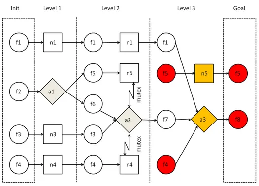
Figure 3.1: An example of inconsistencies in an action plan. Circles rep-resent facts, squares no-ops and diamonds actions. As for colouring, beige marks allowed actions, red unsupported facts, and orange unsupported ac-tions and no-ops.
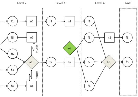
In Figure 3.1, action a2 is mutually exclusive with no-ops n4 and n5. This means that in level 3 both no-op n5 and action a3 have unsupported facts as preconditions. Thus they cannot be performed and if action a2 is the only action that has f 7 as positive effect, it has to exist. The solution to a problem like this could be to add an extra action node a4 with positive effect f 5 and f 4 at level 3, thus pushing both n5 and a3 to level 4. This would turn the latter part of the action graph into Figure 3.2. Since there are no inconsistencies the graph is now a solution graph.
Figure 3.2:An example of how to solve the inconsistencies in Figure 3.1. Cir-cles represent facts, squares no-ops and diamonds actions. As for colouring, beige marks allowed actions and green new actions.
3.4.3
LPG-td Accomplishments
The old version of LPG-td, LPG, was awarded best fully-automated planner at the 3rd IPC in 2002. In [8], LPG is compared against other planners based on planning graphs as well as FF, the winner of the IPC 2. It is shown that LPG can be orders of magnitude faster than the other planners, but that the first solution of LPG can be poor.
Later on, when the LPG-td version was used in IPC4 (2004), it was also awarded as top performer in domains involving "Timed Initial Literals" and in plan qual-ity (in the satisficing planning track)5.
In a more extensive comparison from 2004 (although performed by the de-velopers of LPG-td), when comparing LPG-td against a couple of other planners, LPG-td is the best performer in nearly all the cases6.
5http://zeus.ing.unibs.it/lpg/accessed on 2013-05-03
4
Implementation
The implementation is done by creating the domain and problem file. The do-main file is the core, containing the predicates, functions and actions which to-gether make up the rules of the problem. The problem file lists the objects in one problem instance, initializes them and the function variables and sets the goal specification. In this chapter, the driving assignments are reduced to parcels due to the fact that is is the parcels that have a certain weight, not the assignments.
4.1
Domain File
4.1.1
Types
In the problem there are a three different types: parcels, HDVs, and locations.
4.1.2
Predicates
Predicates are objects that are described using Boolean representation: 1. at(object o, location `)
Description: Object o (HDV or parcel) at location ` 2. in(parcel p, HDV t)
Description: Parcel p in HDV t 3. adjacent(location l1,location l2)
Description: Location l1adjacentto location l2
4. available(parcel p)
Description: Parcel p available (depends on time windows and delivery status)
5. in-use(HDV t)
Description: HDV t in-use (started) 6. goal(parcel p,location `)
Description: Location ` is parcel p’s goal
4.1.3
Functions
Functions are objects with states that can be represented numerically (also called numerical fluents):
1. total-cost
Description: This is the variable that keeps track of the total cost of the solution
2. distance(location l1,location l2)
Description: Metric that keeps track of the distance between l1and l2(only
available for adjacent locations) 3. maxCargo
Description: The maximum cargo limit (the same for all HDVs) 4. cargo(HDV t)
Description: How much weight an HDV t is carrying 5. weight(parcel p)
Description: Parcel p’s weight
4.1.4
Actions
Actions are events that change the state of the problem. In this problem there are four actions possible:
1. useHDV(t)
Description:Sets HDV t as available for use. Precondition:HDV t not in use
Effect: HDV t available 2. load(p, t, l)
Description:Loads a parcel p into HDV t at location `. Precondition:t available, p available, t at `, p at `, cargot+ pw≤maxCap
Effect: p in t, cargot= cargot+ weightp, p not at ` 3. unload(p, t, l)
Description:Unloads a parcel p from HDV t at location `. Precondition:p available, t at `, p in t, p at goal
4.2 Problem File 27
4. moveHDV(t, l1, l2)
Description:Moves HDV t from location l1to l2.
Precondition:t in-use, t at l1, l1adjacent to l2
Effect: t at l2, t not at l1
4.2
Problem File
It is inside the problem file that objects are defined and initialized and the goal is set. This means that a certain domain can have many problem files, which might differ by objects, initial values and goal specifications.
The goal specification is a description of the state that is desired. In the spec-ification, objects are described using the available predicates, and whether they should be true or false. The specification does not have to be complete, e.g., ob-jects that are not listed are considered in goal state from the beginning.
In the problem studied in this thesis, the goal state has been - all parcels at their respective goal location and all HDVs should have returned to their respec-tive origin. The metric to be minimized is called total-cost, and is also set in the problem file. In this thesis total-cost has always been equal to the objective function, which is described in Section 2.6.
5
Evaluation
In this chapter the results of several simulations are presented, together with a description of the problem that is solved in each simulation.
5.1
Definitions
First, a short list with parameters that were used together with LPG-td:
−n n is the maximum number of solutions that can be found
−nobestf irst LPG-td will not use bestfirst
−cputime_localsearch X X is the time spent with hill climbing
−cputime X X is the maximum total time allowed (seconds)
−searchcostx1stsol Total cost will be considered for the first solution as well −noise X X is the noise parameter (0 < X < 1)
−search_steps X X is the number of search steps used
In all the simulations performed, −nobestf irst, −searchcostx1stsol and −noise 0.1 were used, therefore they will not be reported further on.
In all simulations, the costs were specified as:
• Start-up (static) costs — 50 for each vehicle that was "started" i.e., made available for use,
• Driving (dynamic) costs — Driving costs were given by the driving times which equalled driving distance divided by 100.
An important notice that should be made is the difference between found and returned solution value. For a single run, found values consist of all values found
up until a certain time, while the returned value is the best value found for that specific run at that time. Thus;
Returned value ≤ 1 N N X i=1 Found valuei (5.1) Furthermore, the reason why cputime_localsearch always equalled cputime, and nobestf irst were used, was because the best-first algorithm of LPG-td only returned segmentation fault when used. The reason for this might be that the algorithm is based on the fast-forward 1planner, which does not support the use of multiple metrics.
The computer that was used to perform all simulations was a Dell Optiplex 780, with an Intel Core 2 Duo CPU E8400 (3.0 GHz). The simulations were per-formed within a virtual machine given 1024 MB of RAM and running Ubuntu.
5.2
Different Planners
The relative performance of LPG-td was measured by comparing the solutions it found against the solutions of fast-downward. Since fast-downward does not support the same PDDL version as LPG-td, a relaxed problem was used.
The problem that was used included 12 locations, one vehicle at each location and 33 assignments. The relaxed rules were set as follows:
• A vehicle is either empty or full (1 parcel), thus parcel weight is not consid-ered,
• No weights meant that performing more than one assignment at a time was no longer possible. This changed the formula for the fill-rate into
, Fill − rate =T otal distance driven with cargo
T otal distance driven (5.2)
• All time windows are disregarded.
An unfortunate circumstance was that the A* method of fast-downward could not find a solution for the size of problem that was used in the comparison. Thus, two different heuristics for the fast-downwards best-first planner were used to repre-sent fast-downward: "fast forward heuristics" —ff and "context-enhanced addi-tive heuristics" — cea 2. LPG-td entered both with the planner LPG-td but also with LPG-td* ; where LPG-td* is the solution found by LPG-td post-processed to optimize the route found. For example if a vehicle took a driving assignment between location 1 and 4, if LPG-td did not find the route with shortest distance,
1http://fai.cs.uni-saarland.de/hoffmann/ff.html accessed on 2013-05-02 2http://www.fast-downward.org/HeuristicSpecification accessed on 2013-04-23
5.2 Different Planners 31
this was corrected. Worth noting is that fast-downward with theff heuristics al-ways used the shortest distance.
The fast-downwards best-first heuristics are deterministic, and will always find the same result. However, since LPG-td uses hill climbing which is non-deterministic, LPG-td had 10 runs solving the problem with a maximum time limit of 10 000 seconds. The median solution was used for post-processing and when comparing the two planners.
In Figure 5.1, the costs for the different planners are visualized. LPG-td and LPG-td* both beat the competitor fast-downward, LPG-td* with about 10 %. The disappointment in the test was fast-downward with cea heuristics, which per-formed considerably worse than the other three.
To further underline the results from Figure 5.1, the fill-rates are studied in Figure 5.2. Fast-downward with cea heuristics was well beaten by both LPG-td versions, while theff heuristic was a close competitor. An interesting result was that when comparing LPG-td* and LPG-td, LPG-td* produces a better result in Figure 5.1 while the fill-rate was lower, as seen in Figure 5.2.
The distance driven empty is studied in Figure 5.3, and here it is seen why the cea heuristics produces such poor results in this test, when it used almost 3 times the distance of LPG-td’s both versions. Noticeable is also that LPG-td and LPG-td* produced the same result,which means that LPG-td chose the shortest routes between two locations when going empty.
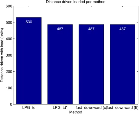
In Figure 5.4, the distance driven with a load is studied, and it is seen where LPG-td loses out versus LPG-td*. With post-processing LPG-td* was able to reduce the driven distance with cargo by 8 %. Noticeable is that the two fast-downward versions chose the shortest routes between locations when they were going with cargo.
LPG−td LPG−td* fast−downward (c)fast−downward (ff) 0 200 400 600 800 1000 1200 832 789 1123 856 Method
Total cost (units)
Total cost per method
Figure 5.1: The total cost connected to the solution of each method, lower cost is better
5.2 Different Planners 33 LPG−td LPG−td* fast−downward (c)fast−downward (ff) 0 10 20 30 40 50 60 70 80 74 % 72 % 48 % 66 % Method Fill−rate (%)
Fill−rate per method
Figure 5.2:The achieved fill-rates for the different methods
LPG−td LPG−td* fast−downward (c)fast−downward (ff) 0 100 200 300 400 500 600 186 186 520 253 Method
Distance driven empty (units)
Distance driven empty per method
Figure 5.3:The distance each method was driving empty, shorter distance is better
LPG−td LPG−td* fast−downward (c)fast−downward (ff) 0 100 200 300 400 500 600 530 487 487 487 Method
Distance driven with load (units)
Distance driven loaded per method
Figure 5.4:The distance each method was driving with load, shorter distance is better
5.3
LPG-td Scaling
The scaling of LPG-td was studied through a set of tests where the problem size increased. The variables that were increased were the number of assignments, vehicles and locations. The objective value and the time it took to find every solu-tion was plotted against the increased variable, and a least-square approximasolu-tion curve of second order was superimposed.
The problems were auto-generated at given sizes, where one variable was in-creased while the other two were held static. The simulation was performed with LPG-td allowed to run the 28 auto-generated problems 8 times for each problem, and after that the mean of the runs was extracted and used in the figures.
Execution parameters
−n 100
−cputime_localsearch 300
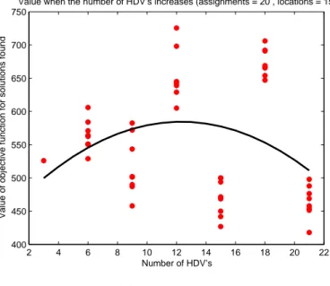
5.3 LPG-td Scaling 35 2 4 6 8 10 12 14 16 18 20 22 400 450 500 550 600 650 700 750
Value when the number of HDV’s increases (assignments = 20 , locations = 15)
Number of HDV’s
Value of objective function for solutions found
(a)Solution values
2 4 6 8 10 12 14 16 18 20 22
0 50 100 150
Solution time when the number of HDV’s increases (assignments = 20 , locations = 15)
Number of HDV’s
Solution time for solutions found
(b)Solution times
Figure 5.5:The objective function value as the number of vehicles increase. The number of vehicles varies between 3 to 21, number of assignments = 20, locations = 15
In Figure 5.5b it is noted that the most difficult problem to solve was when the number of vehicles was small (3 HDVs). With only 3 HDVs LPG-td could only
find 1 solution. When the number of vehicles was increased, the average time to find a solution decreased. As for solution value, differences in solution value did not show any obvious pattern to say that an increase of vehicles (more than the necessary number) affect it.
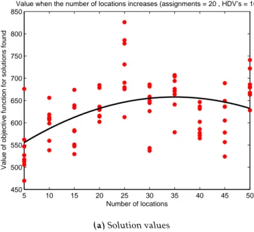
In Figure 5.6b it is noted that all problems were very easy to solve, no matter how many locations were used. Differences in solution value did not show any obvious pattern to say that an increase of locations affects it.
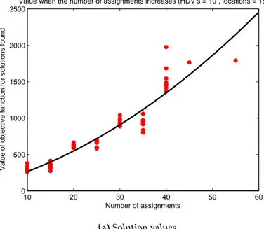
In Figure 5.7b it is noted that the most difficult problems to solve were the ones where the number of assignments were large. When the number of assign-ments increased, the time to find the solutions increased, with what looks to fit a curve of second degree. As for solution value differences in solution value suggest that the number of driving assignments has a high impact on the objective value.
5.3 LPG-td Scaling 37 5 10 15 20 25 30 35 40 45 50 450 500 550 600 650 700 750 800 850
Value when the number of locations increases (assignments = 20 , HDV’s = 10)
Number of locations
Value of objective function for solutions found
(a)Solution values
5 10 15 20 25 30 35 40 45 50 0 20 40 60 80 100 120 140 160 180 200
Solution time when the number of locations increases (assignments = 20 , HDV’s = 10)
Number of locations
Solution time for solutions found
(b)Solution times
Figure 5.6:The objective function value as the number of locations increase. The number of locations varies between 5 to 50, number of assignments = 20, vehicles = 10
10 20 30 40 50 60 0 500 1000 1500 2000 2500
Value when the number of assignments increases (HDV’s = 10 , locations = 15)
Number of assignments
Value of objective function for solutions found
(a)Solution values
10 20 30 40 50 60 0 50 100 150 200 250 300 350
Solution time when the number of assignments increases (HDV’s = 10 , locations = 15)
Number of assignments
Solution time for solutions found
(b)Solution times
Figure 5.7: The objective function value as the number of assignments in-crease. The number of assignments varies between 10 to 60, number of ve-hicles = 10, locations = 20
5.4 LPG-td Performance 39
5.4
LPG-td Performance
The performance of LPG-td was measured by solving the same problem instance 800 times with the following parameters:
−n 10
−cputime_localsearch 60
−cputime 60
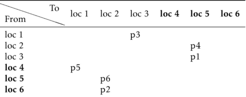
The problem was specified with 6 driving assignments, 6 locations and a maxi-mum of 3 vehicles. P P P P P P PP From To
loc 1 loc 2 loc 3 loc 4 loc 5 loc 6
loc 1 p3 loc 2 p4 loc 3 p1 loc 4 p5 loc 5 p6 loc 6 p2
Table 5.1: Driving assignments between locations, bold marks location where a vehicle starts
This resulted in 4654 solutions to the same problem, and the results is shown in Figures 5.8 to 5.11. In Figure 5.8 the results are plotted against time, with Fig-ure 5.8b showing the same plot zoomed in on the results returned up until 1 second. It is clearly visible that a local minimum exists at value 218 where a lot of solutions processes got stuck. However, there were also solution processes that found the local optima with a value of 168. In Figure 5.9 the mean values returned are plotted.
The difference between found and returned values are clearly visible when comparing Figures 5.10 and 5.11. The number of best solutions found converges at about 9 % of the total solutions (after 10 seconds), but the probability that the solution with value 168 has been returned is more than 90 %. Worth noting is that after 2 seconds the chance of having found the best solution is 50 %, but the planner had already found 3959 solutions out of 4654 (85 %). This means that a lot of the best solutions are found among those in the very end.
0 2 4 6 8 10 12 150 168 178 200 218 250 300 350 400 450 Time (s) Value
Values found in each iteration and time
Iteration 1 Iteration 2 Iteration 3 Iteration 4 Iteration 5
(a)Solution values per iteration and time
0 20 40 60 80 100 150 168 178 200 218 250 300 350 400 450 Time (1/100 s) Value
Values found in each iteration and time
Iteration 1 Iteration 2 Iteration 3 Iteration 4 Iteration 5
(b)Solution values per iteration and time (zoomed in on area 0 to 1 s)
Figure 5.8: The solutions found for the problem as a function of time (and sorted by iteration). Figure 5.8b is zoomed in on the area from 0 to 1 second
5.4 LPG-td Performance 41 0 2 4 6 8 10 160 170 180 190 200 210 220 230 Time (s) Value returned
Mean values returned as a function of time
Figure 5.9:The mean values returned as a function of time
0 2 4 6 8 10 0 1 2 3 4 5 6 7 8 9 10
Percent of solutions found that are the best (168), as a function of time
Time (s)
Found solutions with best value (168) (%)
Figure 5.10:Number of solutions (in percent) equal to the smallest minima found using LPG-td
0 2 4 6 8 10 10 20 30 40 50 60 70 80 90 100 Time (s)
Probability that returned value is best value (%)
Probability (in %) that returned value is best value as a function of time
Figure 5.11:The probability (in percent) that the returned value is equal to the smallest minima found using LPG-td
5.5
LPG-td Relative Improvement
Further simulations were performed to determine the performance of LPG-td. Different problems of the same size were auto-generated using the code in Ap-pendix A. 20 problems were created and solved using the search parameters
−n 10
−cputime_localsearch 1800
−cputime 1800
The solutions were compared to the first solution found for each of the problems, and plotted in Figure 5.12 together with a least-square approximation. In it is clearly visible that the relative improvement seems to converge at about 50 % after around 5 seconds.
5.6 Case Study Problem 43 0 2 4 6 8 10 0 10 20 30 40 50 60 70 Time(s)
Relative improvement compared to the first solution(%)
Relative improvement of solutions (compared to the first solution) depending on time Data points
y=0.0725ln(x)+0.3664
Figure 5.12: Figure showing the relative improvement (in percent) of solu-tions compared to the first solution found. A least-square fit is also visible
5.6
Case Study Problem
The problem that was used to validate LPG-td as a planner for the vehicle routing problem was created based on data obtained from real-life driving assignments and relevant logistic statistics [17], [16]. The case study problem consists of 15 locations, a maximum of 20 vehicles, 4 transport companies (and depots) and 45 assignments. The simulations were performed 10 times for every one of the individual companies as well as for the collaboration, and then the mean was cal-culated and used.
The settings of the case study problem were constructed according to the pat-tern recognized in the data obtained, for example the time windows seemed to be tighter for shorter assignments, thus this was reflected with time windows vary-ing between 2-4 times the drivvary-ing time of each assignment. The drivvary-ing times were calculated by dividing the travel distance by 100. This was done to simulate an average velocity of 100 km/h, although it was a simplification since the aver-age speed of an HDV is typically 80-85 km/h.
com-panies, and the companies were placed in 4 locations (Stockholm, Göteborg, Västerås and Gävle). When the assignments were handed out, consideration was taken to the geography of the origin and destination of the assignment together with the location of each company. A maximum number of vehicles was designated to each company, with Stockholm having 4, Göteborg 5, Västerås 6 and Gävle 5.
Maximum cargo to be held by a single vehicle was set to 40 tonnes, and the volume for assignments was disregarded. The parcels were given weight between 1-25 tonnes each, with a distribution that was inspired by the data obtained.
Worth noting is that even though the problem was based on real-life data, the results should only be used to compare differences between the two different so-lutions: the collaboration and the sum of the individual companies.
Execution parameters for solving the individual problems:
−n 100
−cputime_localsearch 10000 −cputime 10000
Execution parameters for solving the collaboration problem:
−n 100
−cputime_localsearch 50000 −cputime 50000
The full specifications for the case study problem can be found in Tables B.1 to B.5, and a map of the geographical locations used can be found in Figure B.1.
5.6 Case Study Problem 45 1 2 0 500 1000 1500 1413.6 1344.6
The sum of individual solutions (left) and the solution for the collaboration (right)
Value for first solution
First solution for the individual companies (left) and for the collaboration (right)
Figure 5.13:The first solutions found for the individual companies and for the collaboration. The objective value is compared between the two, with lower value being better
In Figure 5.13 it is shown that the planner found an initial solution to the global problem with a value on the objection function that was better than the sum of the individual ones. However, a big difference in computing time should be noted, see Table 5.2, but nevertheless the first solution for the collaboration was 4.9 % better than the first individual solution.
The best solutions found are examined in Figure 5.14, where it is obvious that LPG-td failed to produce a better solution for the collaboration, and the sum of the best found solutions for the individual companies was better by 21.7 %.
In Tables 5.2 and 5.3 the mean of the ten results are shown. An important note to make is that although the time difference in Table 5.3 is not that large, the time it took for the individual solution to reach a result better than the best found for the collaboration was roughly 1000 seconds.
1 2 0 200 400 600 800 1000 1200 910.7 1163.7
The sum of individual solutions (left) and the solution for the collaboration (right)
Value for best solution
Best solution for the individual companies (left) and for the collaboration (right)
Figure 5.14: The best solutions found for the individual companies and for the collaboration. The objective value is compared between the two, with lower value being better
Table 5.2:The first solutions found for the individual companies and for the collaboration
Solution value Time (s) Fill-rate (%) HDVs used
Individual 1413,6 7,364 15,8 17,4(20)
Collaboration 1344,6 1367,755 16,8 16(20)
Table 5.3:The best solutions found for the individual companies and for the collaboration
Solution value Time (s) Fill-rate (%) HDVs used
Individual 844,7 29740,21 19,6 10,1(20)
Collaboration 1127,1 44951,88 16,8 13,6(20)
Another simulation was performed to determine whether the planner only had difficulties decreasing the number of vehicles in the collaboration setting.
5.6 Case Study Problem 47
This was done through an analysis of the ten best solutions for the collaboration; the ten most used vehicles were then made available for use while the other ten were removed. Another simulation, where the ten vehicles used in the individual solutions were made available, was also used.
The result of letting the planner work on both simulations with the following parameters:
−n 100
−cputime_localsearch 200000 −cputime 200000 −search_steps 2000 was that no solution was found.
6
Conclusions
The conclusion that could be made by looking at the simulation of the case study problem, in Section 5.6, was that LPG-td might not be considered as a candidate for solving this type of problem, not with the problem sizes expected, and not with the aim of improving the solutions the individual companies would find themselves.
In Table 5.3 it was shown that for the collaboration, the solution is not only worse by more than 20 %, it also uses more computing time and HDVs. Further on, the fill-rate is lower for the collaborative solution. The problem was too com-plex for LPG-td to be able to produce a better solution for the collaboration, even though — in theory — the solution for the collaboration should always be better, or equal, to the sum of individual solutions.
The scaling of LPG-td was evaluated through multiple simulations, and the result of these are shown in Figures 5.5 to 5.7. Through these simulations, it was possible to suggest that the variation of HDVs and locations did not affect the planner with a noticeable result. The increase of assignments however increased the solution complexity, in terms of both value and time.
LPG-td was also compared to a second planner based on PDDL, fast-downward. In Figures 5.1 to 5.4 it is shown that for the problem that was studied, LPG-td outperformed fast-downward. The fact that fast-downward only could be used with a relaxed problem also contributed to the choice of LPG-td as the planner used in this thesis. An interesting notice is that LPG-td*, a post-processed version of LPG-td, gave a better result when comparing costs, compared to LPG-td. At the same time, LPG-td* achieved a lower fill-rate than LPG-td. This meant that the proposition that the fill-rate should be increased as the costs were decreased
does not hold.
The performance of LPG-td was examined in Figures 5.8 to 5.12. In Figure 5.8 it was shown that a lot of the solutions found by LPG-td were suboptimal, and in Figure 5.11 that it took roughly 2 seconds to have a 50 % chance that the re-turned value was the best. After 2 seconds the planner had already found 3959 solutions out of 4654 (85 %). This meant that LPG-td did not find the best solu-tions until very late in the solving process. In Figure 5.12 it was shown that the solutions converged at about a 50 % improvement compared to the first solution.
To sum it up:
• LPG-td might not be considered a possible candidate for a software that has the goal of optimizing the transport planning for a collaboration of small transport companies.
• Since LPG-td did not produce a better result for the collaboration, nothing could be said whether the result would be adequate to attract customers. • Decreased cost does not have to mean increased fill-rate, but they correlate
7
Discussion
7.1
Transport and Solving Problems
The first part of the discussion relates to the problems of logistics and solving the VRP.
7.1.1
Choice of Planner
The reason why I chose LPG-td is mainly because of the good support (PDDL-wise) but also because as seen in Figure 5.1 the performance of LPG-td is quite good. The downside about it is the scaling performance and that the best-first algorithm used does not support more than one numerical variable. This means that for difficult problems like the final problem treated in this project, the plan-ner returns a segmentation fault when it changes approach to best-first. This is avoided by forcing the planner to use hill climbing for the total available time. The developers have been contacted and as a result they are considering replac-ing the best-first algorithm to the one used in fast-downward.
The existing alternatives (such as fast-downward) currently do not allow the same version of PDDL, meaning that for example fast-downward only supports the use of one numerical expression (defined astotal-cost). In the problem
de-scribed in this project, the need for more numerical variables such as the assign-ment weights in combination with the current cargo and maximum cargo for the HDVs is needed for the capacity constraints. One could manipulate the domain file, emulating numerical expressions using Boolean ones, but according to the author of fast-downward, Malte Helmert, this is not recommended above figures ranging from 1 to 10 and it has not been tested in this project.
7.1.2
Understanding How the Planner Works Versus Usability
A trade-off when using PDDL and the pre-developed planners that are available is that even though it is easy to get started, to write the domain and problem files and apply a planner, it is not easy to understand how the planner actually works. For example for the planner used in this thesis, LPG-td, there exists only as an executable. However, there are numerous papers written on this topic, but since these planners are developed by people with lots of experience and knowledge within the field of planning and optimization, it is still not trivial to understand the way the planners work.7.1.3
Heuristics
The trade-off with using PDDL and automated planners is that to be automated, the planners have to have heuristics that work with all kinds of problems, i.e., they are not problem-specific. Even though the developers of the planners are very experienced and qualified for this task, this means that when using a plan-ner for one specific problem, for example a logistic optimization problem, the performance might suffer from the fact that the planner is not optimized for such a problem. In the literary study it seemed that there were people solving very large problems in good fashion using software that has been tailored for the specific problem, for example in [14].
7.1.4
Soft Constraints
In the problem description it is stated that one assumption is that there are no soft constraints. The meaning of this is that all constraints need to be fulfilled to make a solution acceptable. In real life one could however imagine the use of soft constraints, and the possible consequences. For example one such soft constraint could be the time windows.
The system might be such that the time windows are accompanied by a cer-tain predetermined penalty that is applied if the time window constraint is not met. This is used frequently in different situations such as when constructing buildings etc. This means that it might be accepted to complete an assignment after the latest delivery, but a charge will be taken (alternatively the payment will be reduced). This would introduce several new aspects to consider, and increase the problem complexity vastly.
7.1.5
Adaptivity of PDDL
One of the advantages with using PDDL, is the adaptivity of the planners devel-oped for it. Since the planners do not accept any input heuristics, if the problem can be written for PDDL the planner takes care of the rest.
This means that the possibly very complex task of inventing suitable heuris-tics for a problem can be avoided, and that time can be spent on for example
![Figure 1.1: Swedish fleet sizes 2011 [11]](https://thumb-eu.123doks.com/thumbv2/5dokorg/4650326.120822/8.701.144.574.137.586/figure-swedish-fleet-sizes.webp)