Mälardalen University Press Licentiate Theses No. 251
RESTRUCTURED DISTRICT HEATING PRICE MODELS
AND THEIR IMPACT ON DISTRICT HEATING USERS
Jingjing Song 2017
School of Business, Society and Engineering
Mälardalen University Press Licentiate Theses
No. 251
RESTRUCTURED DISTRICT HEATING PRICE MODELS
AND THEIR IMPACT ON DISTRICT HEATING USERS
Jingjing Song
2017
Copyright © Jingjing Song, 2017 ISBN 978-91-7485-311-7
ISSN 1651-9256
Acknowledgements
I would like to thank my supervisors Prof. Björn Karlsson, Dr. Fredrik Wallin and Dr. Hailong Li for their guidance and support which helped me to formu-late and improve my research over the last three years. My mentors Jan Andhagen and Anders Tenggren from Mälarenergi AB and Mikael Söderberg from Bostads AB Mimer, for their insights and instruction within the topic, which energized and drove my research. My colleagues Claes Erixzon and Stefan Ekström from Mälarenergi AB, for their help with the consumption data that is so important for my research. My peer PhD candidates from Reesbe and MDH, for the interesting discussions, which brought me out of my lonely bubble when my research was at a standstill. My husband Jing Wang and my dear friends, for their support and encouragement during this challenging process.
This thesis is based on work conducted within the industrial post-graduate school Reesbe – Resource-Efficient Energy Systems in the Built Environ-ment. The projects at Reesbe are aimed at key issues in the interface between the business responsibilities of different actors in order to find common solu-tions for improving energy efficiency that are resource-efficient in terms of primary energy and have low environmental impact.
The participating research groups are Energy Systems at the University of Gävle, Energy and Environmental Technology at Mälardalen University, and Energy and Environmental Technology at Dalarna University. Reesbe is an effort in close co-operation with the industry in the three regions of Gävleborg, Dalarna, and Mälardalen, and is funded by the Knowledge Foundation (KK-stiftelsen).
Summary
District heating (DH) is considered to be an efficient, environmentally friendly and cost-effective method for providing heat to buildings, since electricity is usually co-generated in biomass fuelled combined heat and power (CHP) plants. This gives it an important role in the mitigation of climate change. Swedish district heating companies are currently facing multiple challenges, and are in urgent need of new price models to increase transparency and main-tain their competitiveness.
This thesis describes a survey carried out to understand the structure of the present price models and subsequently proposes and compares two restruc-tured price models with the most commonly used price model. This work also investigates the impact of restructured price models on users who would en-counter a significant cost increase if the restructured price models were to be introduced. The district heating costs of different price models are compared with three alternative technical solutions.
The results show that price models based on the consumption pattern of users can reflect district heating companies’ cost structure. Meanwhile, adopt-ing a pricadopt-ing strategy based on users’ consumption patterns increased the in-centives to reduce the peak load.
Consequently, users with high load factor (flat consecutive load curve) were able to reduce costs whereas users with low load factor (steep consecu-tive load curve) faced possible cost increases, when the load demand cost was changed to daily or hourly peak demand based methods. Further, the most economically preferable option for the invested district heating user was to combine district heating with direct electrical heating or with a ground source heat pump.
Sammanfattning
Fjärrvärme anses som ett effektivt, miljövänligt och kostnadseffektivt sätt att leverera värme eftersom kraftvärme blir vanligare i fjärrvärmesystem, där elektricitet produceras tillsammans med värme. Den spelar en viktig roll i att begränsa klimatförändringen. Svenska fjärrvärmeföretag står inför flera utma-ningar nu för tiden, och är i akut behov av nya prismodeller för att öka öppen-heten och behålla konkurrenskraften.
I denna avhandling genomförs en undersökning för att ta reda på strukturen för de nuvarande prismodellerna. Därefter föreslås två omstrukturerade pris-modeller, vars påverkan på kostnaden för fjärrvärmekonsumenterna analyse-ras jämför med den nuvarande modellen.
Detta arbete undersöker också effekten av omstrukturerade prismodeller för konsumenter som skulle drabbas av en signifikant kostnadsökning i sam-band med införandet av dessa prismodeller. Kostnaden för fjärrvärme vid olika prismodeller har också jämförts med tre olika tekniska lösningar.
Resultatet visar att prismodeller som baseras på konsumenters förbruk-ningsprofil kan återspegla fjärrvärmeföretagens kostnadsstruktur; samtidigt medför en prissättningsstrategi baserad på användarens förbrukningsprofil högre incitament för att minska spetseffekten.
Följaktligen kommer konsumenter med stabila konsumtionsprofiler att sänka sina kostnader, medan konsumenter med spetsiga konsumtionsprofiler kommer att drabbas av en kostnadsökning. Vidare är det ekonomiskt mest lön-samma alternativet för den som investerat i fjärrvärme att kombinera fjärr-värme med direkt eluppvärmning eller med en bergfjärr-värmepump.
List of papers
This thesis is based on the following papers, which are referred to in the text by their Roman numerals.
I. Song, J., Wallin, F., Li, H., Karlsson, B. (2016) Price models of dis-trict heating in Sweden. Energy Procedia, 1(2):3–4
II. Song, J., Li, H., Wallin, F. (2016) District heating cost fluctuation caused by price model shift. Applied Energy, accepted.
III. Song, J., Wallin, F., Li, H. (2016) Cost comparison between district heating and alternatives during the price model restructuring process.
International Conference on Applied Energy, Oct. 2016, Beijing,
China. My contributions:
Paper I: survey design, data collection and compilation, and most of the writing.
Paper II & III: all calculations and most of the writing. List of papers not included:
Lundström, L., Song, J. Seasonal Dependent Assessment of Energy Conservation within District Heating Areas. The 14th international
symposium on district heating and cooling, Sep. 2014 Stockholm,
Contents
1 INTRODUCTION ... 1
1.1 Background ... 2
1.2 Cost Structure and Price Model ... 3
1.3 Previous Research ... 3
1.4 Research Questions ... 4
1.5 Outline and Objectives ... 4
1.6 Scope and Delimitation ... 4
2 PRICE MODEL SURVEY ... 6
2.1 Data Collection ... 6
2.2 The Components of Price Models ... 6
2.2.1 Fixed Component ... 6
2.2.2 Load Demand Component ... 7
2.2.3 Energy Demand Component ... 8
2.2.4 Flow Demand Component ... 10
2.3 Share of Different Components ... 10
3 IMPACT OF RESTRUCTURED PRICE MODELS... 12
3.1 Reference and Restructured Models ... 12
3.1.1 Reference Model ... 12
3.1.2 Restructured Model I ... 13
3.1.3 Restructured Model II ... 14
3.2 Sensitivity Study ... 15
3.3 Other Prerequisites and Assumptions ... 15
3.4 The Impact of Restructured Models ... 16
3.4.1 Impact of Restructured Model I ... 17
3.4.2 Impact of Restructured Model II ... 19
3.5 The Impact of Share of Different Components... 20
3.5.1 The Sensitivity Study of Reference Model ... 20
3.5.2 Sensitivity study of Restructured Model I ... 22
3.5.3 The sensitivity study of Restructured Model II ... 24
4 POTENTIAL SOLUTIONS TO LIMIT COST INCREASES ... 26
4.1 User Selection ... 26
4.2 Potential Solutions and Assumptions ... 27
4.3 Feasibility of Potential Solutions ... 28
5 DISCUSSION... 31
6 CONCLUSIONS AND FUTURE WORK ... 32
6.1 Conclusion ... 32
6.2 Future Work ... 33
REFERENCES ... 34
List of figures
Figure 1. Fuels used in district heating production 1980–2015. ... 2
Figure 2. Fixed fee in Gothenburg Energy’s price model. ... 7
Figure 3. Different types of Load Demand Component. ... 8
Figure 4. Different types of Energy Demand Component. ... 9
Figure 5. Monthly district heating consumption of the typical house. ... 11
Figure 6. Share of different price components, 159 price models included. ... 11
Figure 7. Proposed price models and sensitivity cases. ... 13
Figure 8. The cost fluctuation caused by restructured models. ... 17
Figure 9. Number of users experience certain range of cost fluctuation under restructured models. ... 18
Figure 10. Standardized consecutive load curve (daily average) of two customers, facing cost increase and decrease respectively. ... 19
Figure 11. Standardized consecutive load curve (hourly average) of two customers, facing cost increase and decrease respectively. ... 20
Figure 12. The cost fluctuation in different sensitivity cases under the Reference Model. ... 21
Figure 13. Number of users experienced certain range of cost fluctuation under different sensitivity cases of the Reference Model. ... 22
Figure 14. The cost fluctuation in different sensitivity cases under the Restructured Model I. ... 23
Figure 15. Number of users experienced certain range of cost fluctuation under different sensitivity cases of the Restructured Model I. ... 23
Figure 16. The cost fluctuation in different sensitivity cases under the Restructured Model II. ... 24
Figure 17. Number of users experienced certain range of cost fluctuation under different sensitivity cases of the Restructured Model II. .. 25
Figure 18. Standardized consecutive load curve of nine different users with the most increased cost. ... 26
Figure 19. Consecutive load curve of different heating solutions, Restructured Model I as an example. ... 27
Figure 20. Annual cost of district heating and alternative solutions under Reference Model. ... 28
Figure 21. Annual cost of district heating and alternative solutions under Restructured Model I. ... 29
Figure 22. Annual cost of district heating and alternative solutions under Restructured Model II. ... 30
List of tables
Abbreviations
CMC Commercial buildings DEH Direct electrical heating DH District heating
EDC Energy Demand Component FDC Flow Demand Component FxC Fixed Component
GSHP Ground source heat pump
H&S Hospital & Social service buildings IND Industrial buildings
LDC Load Demand Component MFH Multi-family Houses O&S Offices and Schools RM 0 Reference Model RM I Restructured Model I RM II Restructured Model II
Variables
a Interest rate of capital, 3.5%/year.
C Customer’s annual district heating consumption, kWh. Cannual Annuity per installed kilowatt of heat pump, SEK/kW ∙ year. Cb User’s base load, kWh.
Cp User’s peak load, kWh.
Cs User’s summer district heating consumption, kWh. Cw User’s winter district heating consumption, kWh. E The district heating cost of a customer, SEK. Icap Capital investment of heat pump, 15000 SEK/kW. K Assigned consumption hours, hour.
L Lifespan of heat pump, 20 years.
LACH Peak demand calculated based on assigned consumption hour method, kW.
Lpeak User’s peak demand, kW
Penergy Energy price in Reference model, SEK/kWh.
Penergy.b Base energy price (subscribed part) in Restructured Model II, SEK/kWh.
Penergy.p Peak energy price (exceeded part) in Restructured Model II, SEK/kWh.
Penergy.s Energy price during summer season in Restructured Model I, SEK/kWh.
Penergy.w Energy price during winter season in Restructured Model I, SEK/kWh.
Pload Load demand price, SEK/kW.
α The subscription level, proportion of base load plant’s capacity compared with system’s total capacity, %.
1
1 Introduction
A District Heating (DH) system is a centralized system that distributes steam/hot water through a pipe network to satisfy end-users’ heat demand. The centralized heat generation includes benefits such as the possibility to uti-lize energy resources that are otherwise difficult to use (e.g. domestic waste, waste heat from industrial processes, etc.) and is equipped with more ad-vanced control over air pollution.
Thus, district heating is considered to be an efficient, environmentally friendly and cost-effective heating method and is playing an important role in the mitigation of climate change. More than 50% of heat needed for space heating in Sweden is currently supplied by district heating.
In spite of their success, district heating companies are facing multiple chal-lenges. According to H. Sköldberg and B. Rydén [1], the heating market is anticipating reductions in energy demand. The demand for district heating is no exception: a warmer climate and improving energy efficiency of buildings will reduce district heating demand [2] since it is closely related to weather conditions such as outdoor temperature [3] and building characteristics. Re-ducing demand will jeopardize district heating companies’ revenues [4].
Conversely, the peak heat demand is becoming even less predictable be-cause of the increasing frequency of extreme weather [5]. In district heating systems, the base load is usually supplied by plants with low operating costs, whereas the peak load is covered by more expensive plants. Volatile and treme peak demand increases the proportion of heat production from the ex-pensive plants, which in turn increases the production cost, and may act as an obstacle to reducing district heating companies’ maintenance costs, hence af-fecting their profits.
Another pressure comes from the tougher and growing competition from other methods of supplying heat [6]. Heat pumps represent an energy efficient technology for heat production. Their coefficient of performance (COP) is usually between 3 and 5, which means that a heat pump can deliver 3 to 5 kWh of heat for every kWh of electricity that it consumes. As the average district heating price in Sweden is similar to the electricity price [7], and users will be able to lower the cost even further by actively managing their consumption pattern in response to fluctuating electricity price in future, district heating is becoming less competitive. Statistics show that more than one million heat pump units were installed in the ten years between 2002 and 2012 in Sweden [8].
2
1.1 Background
The load in a district heating system usually varies according to the outdoor temperature and time of the day. For instance, the heat demand is much higher during cold winter than during the warm summer, and higher in the daytime than at night.
The fluctuation of heat load did not have a large effect on the production cost in the 70s in Sweden, when district heating production was completely dependent on oil [9]. The fuel mix used in district heating systems became much more diverse since the 80s, and in recent years, district heating produc-tion has been dominated by biofuels.
Figure 1. Fuels used in district heating production 1980–2015. Source: Swedish District Heating Association.
Because of the diverse fuel mix, to achieve a higher profit, district heating system usually consist of several plants which use different fuels: the base heat load is normally covered by bio fuel or waste incineration CHP plants, which requires large investments and high maintenance cost but has lower produc-tion cost due to cheap fuels and low taxes; while the peak heat load is usually covered by boilers burning nature gas or oil, which have smaller investments but higher operating costs.
The running order of these plants is based on the criteria that the plant which has the lowest production cost should be put into operation first, fol-lowed by the second cheapest, and so on until the most expensive plant is
0 10 20 30 40 50 60 70 1980 1985 1990 1995 2000 2005 2010 2015 TW h Oil Natural Gas Coal Electrical Boiler Peat Wood Waste Incineration Heat Pump Waste Heat Others
3 operating. Therefore, the production cost fluctuates according to the heat load and the fuel used in base load and peak load plants.
1.2 Cost Structure and Price Model
Costs for district heating companies usually consist of three segments: asset depreciation/investment cost, production related costs (fuel, tax, operation and management), and administration and maintenance costs. The first segment depends on the capacity the district heating system needs to maintain. Gener-ally speaking, the higher the capacity needed to satisfy users’ demand, the higher is the depreciation/investment cost. The second cost segment is directly related to the production and the fuel mix used in production: the more fuel that is consumed in the production, especially in the case of more expensive fuels, the higher is this cost. The third cost segment relates to neither the sys-tem capacity nor the heat production, but depends on the number of employees and the status of the system.
Before the deregulation of the Swedish energy market in 1996, district heat-ing was part of the infrastructure system and was controlled by Swedish mu-nicipalities or the state. There was a limit on the profit district heating compa-nies were allowed to make, and hence the pricing strategy was the cost-plus method [10]. This strategy implies that the manner (in other word, the price model) in which district heating companies charge their customers should re-flect the cost caused by the customer. Despite subsequent deregulation, the majority of district heating companies are still owned by the municipalities and they have continued to apply the cost-plus principle in their price models.
1.3 Previous Research
Plenty of efforts have been made in the area of district heating price models. Other than the general review of different pricing mechanisms [11] by Li et al. It was pointed out in [12] that district heating pricing strategy affect estate owners’ investments on energy efficiency measures.
Individual pricing strategies have also been analysed, for example, the im-pact of marginal cost strategy on energy efficiency measures has been ana-lysed at local system level in [13]; Lundström et al. [14] also anaana-lysed the impact of seasonal pricing on Energy efficiency measures; Zhang et al. [15] and Poredoš & Kitanovski [16] discussed using exergy as an alternative basis for pricing; Pyrko [17] studied the electricity tariff and found that introducing a pricing strategy based on load demand in the electricity price model could motivate users to change their consumption pattern, (or in other words, reduce the peak demand) to reduce their energy expenditure. The same strategy was suggested in [18] for district heating.
4
1.4 Research Questions
Despite all the research mentioned above, the impacts of restructured price models on users’ costs and the possible counter-strategy against undesirable impacts remains unclear. This thesis aims to answer the questions below by investigating the impacts of such models on individual users and user groups: Q1. What are the structures and features of currently used price models? Q2. What are the impacts of restructured price models on the district heating
users’ costs?
Q3. Are there solutions to restrain the impacts of restructured models?
1.5 Outline and Objectives
This thesis consists of four sections. The first section explains the background of the research and raises the research questions. The price model survey in Section 2 is based on Papers I and II, which give a general insight of the struc-ture of currently used price models, answering research question 1. This sec-tion also provides the price models used in the later cost analysis.
Section 3 analyzes the impact restructured price models have on users’ costs, answering the second research question. The major work and results in this section were published in Paper II.
The study in Section 4 is based on Paper III. In this section a user who is likely to encounter significant cost increases is selected for an alternative cost comparison. This section answers the third research question.
Section 5 and 6 are the discussion and conclusion.
Based on the knowledge gaps identified in the literature, the objectives of this thesis are:
To analyse price model restructuring to improve the transparency of heat pricing.
To investigate the effectiveness of using load demand pricing strategy to motivate users to reduce their peak demand.
1.6 Scope and Delimitation
The price model survey was based on information in price lists from 2014. Subsequent shifts and changes in price levels or price models were excluded. The analysis of restructured models was based on users’ real consumption data from 2012, which is considered to be a normal year with respect to lowest and average outdoor temperature.
5 Direct electrical heating, heat pump, and different combinations of these two options and district heating were considered as potential solutions to limit cost increases: other options such as pellet boilers were not considered.
This calculation of potential heating solutions was based on an average electricity price and COP of heat pump, but these actually fluctuate over the year and time of day. One risk is that peak demand coincides with high prices in electricity and low COP due to very cold weather. There were also sugges-tions to introduce load pricing strategy in electricity price in this research [17], but this perspective was not included in the calculations.
Heat storage or on-site operation optimization were also not included. In practice, users can use heat storage or optimize its operation and easily even out the peak demand, and hence compensate for the cost increase induced by the introduced load pricing strategy.
6
2 Price Model Survey
A price model survey was performed and is described in Papers I and II. The survey includes price models used by large district heating companies. The results show that 60% of the price models charge the same price for users’ energy consumption throughout the year and do not contain any component related to consumption pattern.
2.1 Data Collection
Information on 171 price models was collected from the websites of 80 large district heating companies in 2014. These companies accounted for about 85% of the total district heating production in Sweden, and are therefore considered sufficient as representatives of the sector.
2.2 The Components of Price Models
In summary, four distinct components were identified among the investigated price models: Fixed Component (FXC), Load Demand Component (LDC), Energy Demand Component (EDC) and Flow Demand Component (FDC), distinguished by the contributing parameters. Each model contained at least one of these components.
2.2.1 Fixed Component
The Fixed Component represents the necessary cost for a user to remain in the network, such as billing cost, administration and other customer service costs. This also sometimes covers part of the construction cost (to lay the pipeline, etc.) when the user connects to the network.
In most cases, the Fixed Component did not depend on any feature of users’ consumption, but took the form of a specified annual cost. In some cases, it depended on the user’s peak demand, as shown in Figure 2. In the illustrated example, there was no charge for peak demand under 50 kW, 8,500 SEK/year for peak demand between 50 and 100 kW, and so on. 56% of the investigated models included this component.
7
Figure 2. Fixed fee in Gothenburg Energy’s price model.
2.2.2 Load Demand Component
Load Demand Component is used to cover the cost to the district heating com-pany to maintain a certain level of capacity for users’ peak demand, e.g. for investment costs of facilities, etc. Since the capacity reserved for a specific user is related to the user’s peak demand, district heating companies usually set a price for each kW of peak demand (usually in SEK/kW), and use esti-mated or measured peak demand as a parameter to charge users.
Before the installation of smart meters, meters were read manually once a month or several times a year, hence the peak demand of a user remained un-known for decades. District heating companies used users’ consumption from previous years or previous winters to represent how much capacity needed to be reserved. The survey showed that 16% of the price models were still using this approach.
However, different types of buildings can have very distinct consumption patterns. For example, the consumption of a multifamily house is usually more evenly distributed compared with consumptions of offices or commercial buildings, hence the capacity they require differs greatly. Using the total con-sumption directly as a parameter to represent the peak demand is not very fair.
In order to resolve this problem of unfairness, another concept was intro-duced: assigned consumption hours. The basic idea behind this concept was to differentiate different types of buildings by dividing users’ equivalent an-nual consumption (normal year corrected consumption) with an assumed con-sumption time, to get a more reasonable estimate of users’ peak demand.
Different types of buildings were given different amounts of consumption hours, normally 2,100~2,400 hours for multifamily houses and 1,700~1,900 hours for other types of buildings. This method considered different patterns in different types of buildings, but it also had its own defects: it assumed users in the same group had the same consumption pattern, which was not true in
0 20000 40000 60000 80000 100000 0 100 200 300 400 500 600 700 800 Fi xed fe e (SE K) Peak demand (kW)
8
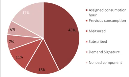
practice. The result of the price model survey showed that 43% of investigated price models used the assigned consumption hour method for the load demand component.
Daily, or even hourly consumption data has become available in recent years, after smart meters which could be read remotely and automatically be-came compulsory for individual users. This development made it possible to introduce pricing strategies based on the individual user’s peak demand, such as the method using measured highest peak demand (11%) or subscribed/ex-ceeded load (6%).
In addition to the methods mentioned above, a further 6% of models used the load signature method. This method uses linear regression analysis of the relationship between the user’s previous daily consumption and the outdoor temperature. The consumption correlation with the extreme low temperature is used to represent the capacity reserved for the user.
These last three methods relate directly to users’ real consumption patterns and could, to some extent, impact the users’ behaviour. However, a full 17% of the price models did not contain a Load Demand Component.
Figure 3. Different types of Load Demand Component.
2.2.3 Energy Demand Component
The Energy Demand Component is used to cover the production cost of dis-trict heating, which is mainly the cost of fuel, taxes and operating costs. All the price models in the survey included an Energy Demand Component which cost each user a certain amount for each kWh of heat consumption.
60% of the surveyed price models used a constant price for the Energy De-mand Component. These models were suitable for systems using a single fuel, implying that the production cost did not fluctuate according to the load level.
43%
16% 11%
7% 6%
17% Assigned consumptionhour
Previous consumption Measured
Subscribed Demand Signature No load component
9 The district heating fuel mix became increasingly diversified after the oil cri-sis, and a constant price was no longer suitable as it could not reflect the real production cost, since district heating systems now had lower production costs at base load and higher production costs at peak load.
Figure 4. Different types of Energy Demand Component.
34% of price models used seasonal price, which was higher during the peak season (usually winter) and lower at other times. This is one way to reflect the production cost and incentivize energy conservation measures that could help to reduce peak demand during the cold season.
However, the most expensive plants are not always in operation during the winter months. Therefore, some companies (1%) set their energy price accord-ing to the outdoor temperature, which is generally a good indicator of the load level in the system and is easily accessed by the general public.
4% of models used a scheme related to the subscribed/exceeded Load De-mand Component. Since only the consumption above the subscription level was charged at a higher price, this method also reflected the cost structure of the energy company.
Some companies experienced difficulties in producing energy at specific times of the day (e.g. in the morning and evening), and lacked sufficient heat storage. To avoid new investment in new heat storage and to encourage users to shift their consumption behaviour, these companies applied a high energy price during the most stressed hours. This type of model accounted for about 0.5% of investigated models. 60% 34% 4% 1% 1% Constant Seasonal Subscribed Outdoor Temperature Peak Period Price
10
2.2.4 Flow Demand Component
About 47% of price models had a Flow Demand Component, which was, in principle, a cost charged according to the volume of hot water needed to fulfil the heat demand of a specific user. This was supposed to cover district heating companies’ pumping costs and sometimes even a portion of the heat losses.
One third of the price models that had a Flow Demand Component used a premium structure. This compares the efficiency of the user’s heat exchanger with the average efficiency in the system. Users are awarded a cost reduction if their heat exchanger has a high efficiency; otherwise, their cost increases. This provides a good motivation for users to improve the efficiency of their heat exchanger.
2.3 Share of Different Components
In addition to the nature of the components, the share of each component is also an important feature of price models, as it affects the magnitude of fluc-tuations in both district heating companies’ income and users’ costs. However, this could not be calculated without more detailed information about the users.
In order to calculate the share of different components in the price models, the same assumptions were made as used in the annual Nils Holgerson cost report, using a typical multi-family house as an example.
The area of the multi-family building is 1,000 m2, consisting of 15 apart-ments;
Annual district heating consumption is 193 MWh, supplied by 3,860 m3 of hot water;
25% of heat is used for domestic hot water, distributed evenly throughout the year;
75% of heat is used for space heating, distributed in proportion to degree-days over a normal year (calculated from Västerås temperature statistics between 1960 and 2014, source: Swedish Meteorological and Hydrologi-cal Institute).
The monthly district heating consumption of the typical house used in the sur-vey was shown in Figure 5.
11
Figure 5. Monthly district heating consumption of the typical house.
Annual costs of 159 price models were calculated based on the above assump-tions. Cost calculations for the other 12 models could not be carried out be-cause daily or even hourly consumption data were required to make the cal-culation, which made the necessary assumptions much more complicated and less trustworthy.
According to the calculation results, Load Demand Component and Energy Demand Component accounted for about 26% and 68% of the cost on average respectively, and were the major components of users’ costs. Conversely, Fixed Component and Flow Demand Component accounted for only 1% and 4% of the annual cost of the typical house respectively. The shares of each component in the collected price models are shown in descending order with respect to share of Energy Demand Component in Figure 6.
Figure 6. Share of different price components, 159 price models included. EDC: Energy Demand Component; LDC: Load Demand Component; FXC: Fixed Component; FDC: Flow Demand Component.
0,0 5,0 10,0 15,0 20,0 25,0 30,0
Jan Feb Mar Apr May Jun Jul Aug Sep Oct Nov Dec
MWh
Domestic Hot Water Space Heating
0% 10% 20% 30% 40% 50% 60% 70% 80% 90% 100% 159 Price Models Average EDC LDC FXC FDC
12
3 Impact of Restructured Price Models
This section evaluates the impact of restructured models by comparing users’ costs before and after the implementation of the new models. The most com-monly used price model (Reference Model, RM0) is used as the baseline, whereas two emerging new price models (Restructured Model I & II, RM I & RM II) are also proposed to calculate the annual cost after new price model implementation. Both Restructured Model I and Restructured Model II con-tain pricing strategies based on users’ actual peak demand.
3.1 Reference and Restructured Models
The results of the price model survey show that Energy Demand Component and Load Demand Component accounted for more than 95% of total cost, whereas Fixed Component and Flow Demand Component accounted for a very small share in existing models. Therefore, the latter two components were not included in these price models.
3.1.1 Reference Model
For the Reference Model (Figure 7a), Load Demand Component and Energy Demand Component were determined by using the assigned consumption hour method and constant energy price respectively. Assigned consumption hour is an assumption made by district heating companies about the number of consumption hours per year (alternatively per winter, typically 2,100~2,400 hours/year for multi-family house and 1,600~1,900 hours/year for other build-ings) in order to determine the user’s peak demand (Eq. 1). The total district heating cost of an individual user was calculated using Eq. 2.
𝐿𝐿𝐴𝐴𝐴𝐴𝐴𝐴 = 𝐶𝐶 𝑘𝑘⁄ (Eq. 1)
LACH: Peak demand calculated based on assigned consumption hour method, kW.
C: Customer’s annual district heating consumption, kWh. k: Assigned consumption hours, hour.
𝐸𝐸 = 𝑃𝑃𝑒𝑒𝑒𝑒𝑒𝑒𝑒𝑒𝑒𝑒𝑒𝑒× 𝐶𝐶 + 𝑃𝑃𝑙𝑙𝑙𝑙𝑙𝑙𝑙𝑙× 𝐿𝐿𝐴𝐴𝐴𝐴𝐴𝐴 (Eq. 2)
E: The district heating cost of a customer, SEK. Penergy: Energy price, SEK/kWh.
13 a) Reference Model b) Restructured Model I
c) Restructured Model II
d) Sensitivity Cases
Figure 7. Proposed price models and sensitivity cases.LDC: Load Demand Component; EDC: Energy Demand Component.
3.1.2 Restructured Model I
Unlike the Reference Model, Restructured Model I (Figure 7b) introduces a pricing strategy based on users’ peak load (on daily basis) to determine Load Demand Component instead of the engineering approximation method, i.e. assigned consumption hour approach. Load Demand Component is charged according to the highest measured daily average demand. For Energy Demand Component, a two-level seasonal energy price is used to differentiate summer and winter consumptions.
This method was able to better reflect the actual production cost than the constant price in the Reference Model, and motivate users to reduce their con-sumption during winter, which is also when the expensive peak load plant comes into operation. A user’s district heating cost is expressed as:
0% 50% 100%
Current
situation EDC only High LDCLDC EDC
14
𝐸𝐸 = 𝑃𝑃𝑒𝑒𝑒𝑒𝑒𝑒𝑒𝑒𝑒𝑒𝑒𝑒.𝑤𝑤× 𝐶𝐶𝑤𝑤+ 𝑃𝑃𝑒𝑒𝑒𝑒𝑒𝑒𝑒𝑒𝑒𝑒𝑒𝑒.𝑠𝑠× 𝐶𝐶𝑠𝑠+ 𝑃𝑃𝑙𝑙𝑙𝑙𝑙𝑙𝑙𝑙× 𝐿𝐿𝑝𝑝𝑒𝑒𝑙𝑙𝑝𝑝 (Eq.3)
Penergy.w: Energy price during winter season, SEK/kWh. Penergy.s: Energy price during summer season, SEK/kWh. Cw: User’s winter district heating consumption, kWh. Cs: User’s summer district heating consumption, kWh. Pload: Load demand price, SEK/kW.
Lpeak: User’s peak demand (daily), kW
3.1.3 Restructured Model II
Restructured Model II, representing another trend of new developments, uses hourly consumption data in the determination of both Load Demand Compo-nent and Energy Demand CompoCompo-nent. It is also based on pricing strategy based on peak demand; however, unlike Restructured Model I, the district heating company suggests a subscription level based on the user’s load de-mand (usually in proportion to measured peak dede-mand). Users thus pay for each kW of subscribed load demand. Since the subscribed level is proportional to peak demand, this method motivates users to limit their peak demand.
The ratio between subscribed and measured peak demand is determined by the ratio between the base load plant and peak load plant capacities in the district heating system. For example, if a district heating system consists of a base load plant with a capacity of 150 MW and a peak load plant with a ca-pacity of 100 MW, this level should be set at 150 MW/(150+100) MW, i.e. 60%. In this analysis, the subscribed load demand was set at 60% of measured peak load, based on the structure of the local district heating system.
The Energy Demand Component consists of two price levels: users are en-titled to pay a lower price (so called base price) for their energy consumption below the subscription level (base load); however, peak energy consumption above the subscription level is charged at a higher price (so called peak price), as shown in Figure 7c. Since the peak price is higher, this method incentivizes users to limit their peak energy consumption. The cost is calculated using the formula below.
𝐸𝐸 = 𝑃𝑃𝑒𝑒𝑒𝑒𝑒𝑒𝑒𝑒𝑒𝑒𝑒𝑒.b× 𝐶𝐶𝑏𝑏+ 𝑃𝑃𝑒𝑒𝑒𝑒𝑒𝑒𝑒𝑒𝑒𝑒𝑒𝑒.p× 𝐶𝐶𝑝𝑝+ 𝑃𝑃𝑙𝑙𝑙𝑙𝑙𝑙𝑙𝑙× 𝐿𝐿𝑝𝑝𝑒𝑒𝑙𝑙𝑝𝑝×α (Eq. 4)
Penergy.b: Base energy price (subscribed part), SEK/kWh. Penergy.p: Peak energy price (exceeded part), SEK/kWh. Cb: User’s base load, kWh.
Cp: User’s peak load, kWh.
Pload: Load demand price, SEK/kW. Lpeak: User’s peak demand (hourly), kW
α: the subscription level, proportion of base load plant’s capacity compared with system’s total capacity, %.
15
3.2 Sensitivity Study
In order to better understand how the share between different components would impact cost to the user, three sensitivity cases were also included in the study:
Case 0: base case (EDC/LDC: 70%/30%), which corresponds to the aver-age share of Energy Demand Component and Load Demand Component among price models in the price model survey. The cost under the Refer-ence Model and the share in this case is used as the baseline for compari-son.
Case 1: Energy Demand Component only (EDC/LDC: 100%/0%), which was considered more straightforward by the users, since the cost to users is proportional to the heat they consume. This case was commonly pre-ferred by users according to the previous survey;
Case 2: high Load Demand Component (EDC/LDC: 55%/45%), which reflects district heating companies’ cost structure. This case was favoured by district heating companies, as it reduces the risks caused by reduced heat demand and secures the intended profit level for district heating com-panies.
3.3 Other Prerequisites and Assumptions
Weather conditions such as the degree days and lowest outdoor temperature have significant impacts on users’ heating consumption and consumption pat-tern. Therefore it is important to find a normal year, during which the condi-tion is close to the historic average.
According to weather statistics from the Swedish Meteorological and Hy-drological Institute (SMHI), the degree days of the year 2012 (3,784 degree days) and the lowest outdoor temperature (-17.3°C) were close to the average historic data between 1985 and 2014 (3,765 degree days, -16.5°C respec-tively), and therefore the data from 2012 were used in this analysis.
The analysis mainly focuses on larger district heating users, which were categorized into five groups: multi-family house (MFH), office & school building (O&S), commercial building (CMC), hospital/social services build-ing (H&S) and industry buildbuild-ing (IND). Smaller users were excluded due to their small share of the total district heating consumption.
To determine the component prices in different price models and sensitivity cases, the total revenue of the district heating company was kept unchanged. Based on this prerequisite, the calculated price levels are listed in Table 1.
16
Table 1. Price-levels of proposed price models
3.4 The Impact of Restructured Models
The cost of district heating for different users was evaluated based on real consumption data. District heating costs calculated using Restructured Models I and II were compared to the cost of the Reference Model. The cost changes resulting from the application of Restructured Models I and II are illustrated in Figure 8.
Case 0
70% / 30% 100% / 0% Case 1 55% / 45% Case 2
Reference Model
Price level for Energy
compo-nent (SEK/kWh) 0.422 0.603 0.332
Price level for Load
compo-nent (SEK/kW) 0.362 0.000 0.543
Restructured Model I Price level for Energy
compo-nent in summer (SEK/kWh) 0.253 0.361 0.199 Price level for Energy
compo-nent in winter (SEK/kWh) 0.455 0.650 0.357 Price level for Load
compo-nent (SEK/kW) 0.560 0.000 0.840
Restructured Model II Price level for Energy
compo-nent base (SEK/kWh) 0.369 0.528 0.290 Price level for Energy
compo-nent peak (SEK/kWh) 1.386 1.979 1.089 Price level for Load
17
Figure 8. The cost fluctuation caused by restructured models. RM I: Restructured Model I; RM II: Restructured Model II; LDC: Load Demand Component; EDC: Energy Demand Component; MFH: Multi-family house; O&S: Office and school; CMC: Commercial building; H&S: Hospital and social service building; IND: Industry building.
3.4.1 Impact of Restructured Model I
Compared to the Reference Model, Restructured Model I had a very limited effect on groups of multi-family houses and office & school buildings, where the cost remained at the same level (99% and 101% respectively). The costs to commercial buildings and industry buildings increased by about 3% com-pared with the Reference Model, and the cost to hospital & social service buildings declined by 4%.
Energy Demand Component in this model depends on heat consumption during winter and summer respectively. As stated in section 3.1.2, since the winter price is higher than the summer price, it is more beneficial to reduce consumption during winter than during summer. Since pricing strategy based on peak demand was also considered, user’s Load Demand Component cost depended solely on actual peak demand (in daily average), hence users could reduce their cost directly by limiting their peak demand.
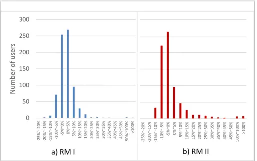
Figure 9a shows the statistical results of cost fluctuations under this model: 1.2% of users faced decreases of 10% or more, 6.7% of users encountered a cost increase of 10% or higher, and 0.5% of users faced a cost increase above 50%.
The total cost depended on the proportion of heat consumption during win-ter and the user’s peak demand, both of which were closely related to the user’s consumption pattern. Therefore individual users’ consumption patterns were examined more closely to understand the impact.
99% 101%103%96%103% 100%104%101% 97% 98% 0% 20% 40% 60% 80% 100% 120%
MFH O&S CMC H&S IND MFH O&S CMC H&S IND LDC EDC
18 0 50 100 150 200 250 300 -2 5% ~-20 % -2 0% ~-15 % -1 5% ~-10 % -1 0% ~-5% -5 %~ 0% 0% ~5 % 5% ~1 0% 10 % ~1 5% 15 % ~2 0% 20 % ~2 5% 25 % ~3 0% 30 % ~3 5% 35 % ~4 0% 40 % ~4 5% 45 % ~5 0% 50 % ~1 00% >1 00% Nu mb er o f u ser s a) RM I -2 5% ~-20 % -2 0% ~-15 % -1 5% ~-10 % -1 0% ~-5% -5 %~ 0% 0% ~5 % 5% ~1 0% 10 % ~1 5% 15 % ~2 0% 20 % ~2 5% 25 % ~3 0% 30 % ~3 5% 35 % ~4 0% 40 % ~4 5% 45 % ~5 0% 50 % ~1 00% >1 00% b) RM II
Figure 9. Number of users experience certain range of cost fluctuation under restructured models.
RM I: Restructured Model I; RM II: Restructured Model II
Individual analysis was performed on two users facing a significant cost in-crease and dein-crease respectively: user 207 from the hospital & social service group, whose annual district heating cost showed the largest decrease; and user 801 from the office & school group, whose cost increased most when Restructured Model I was introduced.
The standardized consecutive load curves of these two users are shown in Figure 10. The x-axis represents the days of the year, the y-axis represents the quotient between instance consumption and average consumption. The curve of user 207 shows less fluctuation than that of user 801.
Correspondingly, the cost of user 207 decreased by 10% when the price model shifted to Restructured Model I, about 9% of which was contributed by the reduced Load Demand Component; whereas the cost of user 801 increased by 216%, where 215% came from the increased Load Demand Component. Assuming user 801 would like to maintain their district heating cost at the same level, they would need to reduce their peak demand by 78%, equivalent to a 50% energy consumption reduction during peak demand periods.
19
Figure 10. Standardized consecutive load curve (daily average) of two customers, facing cost increase and decrease respec-tively.
This cost fluctuation seems suitable since flat curve is good for both district heating companies and the environment, since it contributes to reducing the operation cost and fossil fuel use at peak load production.
3.4.2 Impact of Restructured Model II
Compared to the Reference Model, Restructured Model II had very limited impact on the multi-family house and commercial building groups, whose costs varied by less than 1%, while the office & school group faced a 4% increase and the hospital & social service and industry building groups faced decreases of 3% and 2% respectively.
Under Restructured Model II, users’ district heating costs also depended on the detailed consumption pattern: the Energy Demand Component was deter-mined by both the subscribed consumption and the consumption exceeding the subscribed level, whereas the Load Demand Component was determined by the user’s actual peak demand at hourly resolution.
Comparison of Figure 9a with Figure 9b shows that more users experienced a large fluctuation in cost under Restructured Model II than under Restruc-tured Model I: about 4% of users had a cost decrease of over 10%; 12% en-countered a cost increase higher than 10%; and 1.7% of users enen-countered a cost increase of 50% or higher.
The two users with the largest cost increase and decrease under Restruc-tured Model II were also examined individually. The standardized consecutive load curves for these users, user 793 and user 801, are shown in Figure 11.
0 5 10 15 20 25 30 1 51 101 151 201 251 301 351 Sta nd ar di zed loa d d em an d Day s H&S-207 O&S-801
20
Figure 11. Standardized consecutive load curve (hourly average) of two customers, facing cost increase and decrease respec-tively.
User 793 had the largest cost reduction (12%), 7% from Load Demand Com-ponent and 5% from Energy Demand ComCom-ponent. Contrastingly, for user 801, Energy Demand Component decreased the cost by 7%, but Load Demand Component increased cost by 355%, resulting in a total cost increase of 348%. In order for user 801 to maintain the same cost level, they would have to re-duce their peak demand by 86%, equivalent to a heat consumption reduction of 56% during peak demand periods.
3.5 The Impact of Share of Different Components
3.5.1 The Sensitivity Study of Reference Model
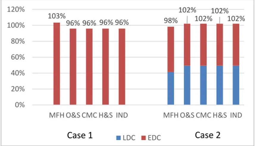
The impacts of Load Demand Component and Energy Demand Component on the energy cost for different user groups are shown in Figure 12. It is clear that for multi-family houses, the energy cost increases with the increase of the share of Energy Demand Component. When the share of Energy Demand Component increases from 70% to 100%, this group’s cost increases by 3%; if the share of Energy Demand Component declines from 70% (Case 0) to 55% (Case 2), this group’s district heating cost decreases by 2%.
However, the share of Load Demand Component and Energy Demand Component affects other groups in the opposite way: when the share of Energy Demand Component increases (from Case 0 to Case 1), all four other groups’
0 10 20 30 40 50 60 1 464 927 1390 1853 2316 2779 3242 3705 4168 4631 5094 5557 6020 6483 6946 7409 7872 8335 Sta nd ad rized lo ad d em an d Ho urs CMC-793 O&S-801 0 1000 2000 3000 4000 5000 6000 7000 8000
21 costs decrease by 4%, where an decline in the share of Energy Demand Com-ponent (from Case 0 to Case 2) increase these four groups’ costs by 2%. This implies that the multi-family house group benefits from a higher share of Load Demand Component under this model.
Figure 12. The cost fluctuation in different sensitivity cases under the Reference Model.
LDC: Load Demand Component; EDC: Energy Demand Component; MFH: Multi-family house; O&S: Office and school; CMC: Commer-cial building; H&S: Hospital and soCommer-cial service building; IND: Industry building.
For the Reference Model, once the assigned consumption hour is determined, the user’s district heating cost depends solely on their annual consumption. Therefore users that have the same amount of assigned consumption hours are affected in the same manner when the share of price model component changes. As shown in Figure 13, when shifted from the base case (Case 0) to Case 1 (Figure 13a), all 356 users from the multi-family house group receive a slight cost increase; whereas when shifted from Case 0 to Case 2 (Figure 13b), 392 users from the other four groups receive a mild cost increase.
103% 96% 96% 96% 96% 98% 102% 102%102%102% 0% 20% 40% 60% 80% 100% 120%
MFH O&S CMC H&S IND MFH O&S CMC H&S IND LDC EDC
22 0 50 100 150 200 250 300 350 400 450 -2 5% ~-20 % -2 0% ~-15 % -1 5% ~-10 % -1 0% ~-5% -5 %~ 0% 0% ~5 % 5% ~1 0% 10 % ~1 5% 15 % ~2 0% 20 % ~2 5% 25 % ~3 0% 30 % ~3 5% 35 % ~4 0% 40 % ~4 5% 45 % ~5 0% 50 % ~1 00% >1 00% Nu mb er o f u ser s a) Case 1 -2 5% ~-20 % -2 0% ~-15 % -1 5% ~-10 % -1 0% ~-5% -5 %~ 0% 0% ~5 % 5% ~1 0% 10 % ~1 5% 15 % ~2 0% 20 % ~2 5% 25 % ~3 0% 30 % ~3 5% 35 % ~4 0% 40 % ~4 5% 45 % ~5 0% 50 % ~1 00% >1 00% b) Case 2
Figure 13. Number of users experienced certain range of cost fluctua-tion under different sensitivity cases of the Reference Model.
3.5.2 Sensitivity study of Restructured Model I
The impacts of Load Demand Component and Energy Demand Component under Restructured Model I are similar to those for the Reference Model (Fig-ure 14). As the share of Energy Demand Component increases (Case 1), costs for the multi-family houses group also increases (3%) while the costs of all other groups falls between 3% and 5%. In the case of high Load Demand Component share (Case 2), multi-family houses’ cost decreases by 1%, the hospital & social services group’s cost remains the same, while the costs of other groups increases by 2% to 3%.
Figure 15 shows the statistical results of cost variation under different sen-sitivity study cases. In Case 1, where Load Demand Component is absent, the majority (ca. 92% of users) only show a slight cost change (±5%), as shown in Figure 15a. As the share of Load Demand Component increases, more users face higher levels of cost fluctuation. In Case 2 (Figure 15b), 3.2% of users have a decrease of 10% or more, whereas 13.1% users face increases of 10% or higher, with the cost for two users doubling. In general, more users benefit from higher share of Energy Demand Component compared to Load Demand Component.
23
Figure 14. The cost fluctuation in different sensitivity cases under the Restructured Model I.
LDC: Load Demand Component; EDC: Energy Demand Component; MFH: Multi-family house; O&S: Office and school; CMC: Commer-cial building; H&S: Hospital and soCommer-cial service building; IND: Indus-try building.
Figure 15. Number of users experienced certain range of cost fluctua-tion under different sensitivity cases of the Restructured Model I. 103% 97% 95% 100% 95% 99% 102%103%100%102% 0% 20% 40% 60% 80% 100% 120%
MFH O&S CMC H&S IND MFH O&S CMC H&S IND LDC EDC Case 1 Case 2 0 50 100 150 200 250 300 350 400 -2 5% ~-20 % -2 0% ~-15 % -1 5% ~-10 % -1 0% ~-5% -5 %~ 0% 0% ~5 % 5% ~1 0% 10 % ~1 5% 15 % ~2 0% 20 % ~2 5% 25 % ~3 0% 30 % ~3 5% 35 % ~4 0% 40 % ~4 5% 45 % ~5 0% 50 % ~1 00% >1 00% Nu mb er o f u ser s a) Case 1 -2 5% ~-20 % -2 0% ~-15 % -1 5% ~-10 % -1 0% ~-5% -5 %~ 0% 0%~5 % 5% ~1 0% 10 % ~1 5% 15 % ~2 0% 20 % ~2 5% 25 % ~3 0% 30 % ~3 5% 35 % ~4 0% 40 % ~4 5% 45 % ~5 0% 50 % ~1 00% >1 00% c) Case 2
24
3.5.3 The sensitivity study of Restructured Model II
The impact of the share of different components is demonstrated in Figure 16. As the share of Energy Demand Component increases (Case 1), the costs to multi-family houses and hospital & social services increases by 6% and 2% respectively, while the costs to other groups fall by 9%, 11% and 7% respec-tively. As the share of Load Demand Component increases (Case 2), the costs to group multi-family house and hospital & social services decrease by 3% and 1% respectively, while the costs to other groups increase by 4%, 6% and 4%respectively.
Figure 16. The cost fluctuation in different sensitivity cases under the Restructured Model II.
LDC: Load Demand Component; EDC: Energy Demand Component; MFH: Multi-family house; O&S: Office and school; CMC: Commer-cial building; H&S: Hospital and soCommer-cial service building; IND: Indus-try building. 106% 91% 89%102%93% 97% 104% 106% 99%104% 0% 20% 40% 60% 80% 100% 120%
MFH O&S CMC H&S IND MFH O&S CMC H&S IND LDC EDC
25
Figure 17. Number of users experienced certain range of cost fluctua-tion under different sensitivity cases of the Restructured Model II.
When the share of Load Demand Component increases (Case 2), 7% of users face cost reductions of more than 10%, 21% of users face cost increases higher than 10%, and 3% of users face cost increases higher than 50%. Whereas for Case 1, fewer users (about 2%) face cost increases higher than 10%, but more users (around 35%) receive cost reductions of more than 10%. Nevertheless, a larger number of users benefit in Case 1, with a higher share of Energy De-mand Component. 0 50 100 150 200 250 300 -2 5% ~-20 % -2 0% ~-15 % -1 5% ~-10 % -1 0% ~-5% -5 %~ 0% 0% ~5 % 5% ~1 0% 10 % ~1 5% 15 % ~2 0% 20 % ~2 5% 25 % ~3 0% 30 % ~3 5% 35 % ~4 0% 40 % ~4 5% 45 % ~5 0% 50 % ~1 00% >1 00% Nu mb er o f u ser s a) Case 1 -2 5% ~-20 % -2 0% ~-15 % -1 5% ~-10 % -1 0% ~-5% -5 %~ 0% 0% ~5 % 5% ~1 0% 10 % ~1 5% 15 % ~2 0% 20 % ~2 5% 25 % ~3 0% 30 % ~3 5% 35 % ~4 0% 40 % ~4 5% 45 % ~5 0% 50 % ~1 00% >1 00% c) Case 2
26
4 Potential Solutions to Limit Cost Increases
The potential of using electrical heating to limit the cost increase when imple-menting the restructured models was investigated by closer examination of a specific user who encountered significant cost increases. The user’s annual costs were calculated under three price models, as well as the cost of three potential solutions, in order to investigate their feasibilities. The study in this section was based on previous work described in Paper III, with some adjust-ments to the assumptions regarding heat pump investment and performance.
4.1 User Selection
Users who encounter significant cost increases after implementing restruc-tured models are more likely to take actions to deal with the changed circum-stances. Hence it is essential for these users and the district heating companies to understand what would be feasible alternatives to district heating.
Figure 18. Standardized consecutive load curve of nine different users with the most increased cost.
X-axis: days of the year, Y-axis: quotient between instance and average district heating consumption.
27 The standardized consecutive load curve of nine users whose costs increased the most are shown in Figure 18. Since User 541 had a typical curve among these users, this user was selected for alternative cost comparisons. The cost of User 541 increased by 35% and 73% under Restructured Models I and II respectfully.
4.2 Potential Solutions and Assumptions
Three solutions were considered in this study. These covered direct electrical heating (DEH) as peak demand and district heating as base demand; base de-mand with ground source heat pump (GSHP) and peak dede-mand with district heating (DH) / direct electrical heating (DEH). Figure 19 shows the consecu-tive load curve and the contribution of each alternaconsecu-tive. The annual cost of each solution is the sum of the district heating cost, electricity cost and annu-ities for heat pump installation. The cost of installing direct electrical heating equipment is assumed to be zero over its 20 year lifespan [19].
Figure 19. Consecutive load curve of different heating solutions, Restructured Model I as an example.
DH: district heating; DEH: direct electrical heating; GSHP: ground source heat pump
28
Different models from the ground source heat pump supplier (NIBE) were used in cost calculations, the model which could achieve the minimum annual cost was chosen. The capital investment for the heat pump was assumed to be 15,000 SEK per installed kilowatt [20], lifespan was assumed to be 20 years, and interest rate was 5% [21]. The annual investment cost of the heat pump was calculated using Eq. 5, which resulted in an annuity of 1,990 SEK / year per installed kilowatt. The SCOP of the ground source heat pump was as-sumed to be 3.5. Price of electricity was asas-sumed to 795 SEK /MWh [22].
𝐶𝐶𝑎𝑎𝑎𝑎𝑎𝑎𝑎𝑎𝑎𝑎𝑎𝑎 = 𝐼𝐼𝑐𝑐𝑎𝑎𝑐𝑐× (1 + 𝛼𝛼) 𝐿𝐿
𝐿𝐿
⁄ (Eq. 5)
Cannual: Annuity per installed kilowatt of heat pump, SEK/kW ∙ year.
Icap: Capital investment of heat pump, 15,000 SEK/kW. a: interest rate of capital, 5%/year.
L: Lifespan of heat pump, 20 years.
4.3 Feasibility of Potential Solutions
If the price model of district heating remains the same (RM 0), the most fea-sible solution would be to install a heat pump to cover the base demand and combine this with district heating to cover the peak demand (Figure 20). This solution was 8% cheaper than the district heating only system. The alternative of using district heating to cover the base demand and adding direct electrical heating to cover the peak did not show any advantages compared with the cost of the district heating only solution. Installing a heat pump to cover the base and combining with direct electrical heating to cover the peak demand cost more than all the other alternatives, increasing the annual cost by 5%.
Figure 20. Annual cost of district heating and alternative solutions under Reference Model.
DH: district heating; DEH: direct electrical heating; HP: heat pump; El: electricity
29 Under Restructured Model I, reducing the peak in the district heating demand with direct electrical heating would be the most economical choice, reducing the annual cost by 31%. Installing a heat pump to cover the base and using direct electrical heating to cover the peak demand would be the second-best alternative. Assuming a 20 year lifespan, this alternative was 25% cheaper compared to a district heating only system. Installing a ground source heat pump to supply base demand and using district heating to cover the peak de-mand would not result in much difference from keeping the district heating as it is, and only reduced the annual cost by 2%. The annual cost of each alterna-tive is shown in Figure 21.
Figure 21. Annual cost of district heating and alternative solutions under Restructured Model I.
DH: district heating; DEH: direct electrical heating; HP: heat pump; El: electricity
On implementing Restructured Model II, the most economical solution is the same as in Restructured Model I: using direct electrical heating to cover the peak demand of district heating. This solution reduced annual cost by about 45% compared with the district heating only system. Installing a heat pump to cover the base demand and combining with direct electrical heating to cover peaks was the second most economical solution, reducing cost by 39%. Con-versely, installing a ground source heat pump to cover the base demand in-stead of district heating increased cost by 4%. The annual cost of three differ-ent alternatives together with the cost of district heating under Restructured Model II is also shown in Figure 22.
30
Figure 22. Annual cost of district heating and alternative solutions under Restructured Model II.
DH: district heating; DEH: direct electrical heating; HP: heat pump; El: electricity
31
5 Discussion
The calculations were based on users’ actual consumption data in a normal year (2012), but impacts related to variations in weather need further investi-gation. One solution could be to develop a weather normalization tool in order to re-generate users’ consumption details.
Neither Restructured Model I nor Restructured Model II could accurately reflect the actual production cost. Seasonal price in Restructured Model I pro-vided one of the best estimates based on previous experiences, but as weather aberrations occur more frequently, the production cost during warm win-ter/cold summer tends to deviate more from the estimated cost. Restructured Model II charges a higher price for users’ peak consumption, but there were some exceptions where the peaks of the users and the system peak did not coincide. The mismatches between district heating price and the actual pro-duction cost indicates that pre-determined price leads to significantly higher financial risk, an effect which has been previously noted in both
[
23] and [24]. A price forecast similar to electricity cost, or real-time price basing on the actual operation could be a plausible alternative.More district heating users benefited from a high share of Energy Demand Component in the pricing models, but this does not necessarily mean this is the right option. The key question here is whether users that help to increase the efficiency of the district heating system benefit from the high share of En-ergy Demand Component. Therefore, a closer investigation is needed at the individual level. The load factor or standardized consecutive load curve could be useful indicators to identify users preferred by district heating companies and to find out whether they benefit from this kind of shift.
32
6 Conclusions and Future Work
6.1 Conclusion
Four price model components were identified in the price model survey. These components contains different approaches in order to improve the transpar-ency of price models so that users are charged based on their actual consump-tion pattern instead of based on the energy companies’ previous experience or engineering approximation.
Pricing strategies based on the users’ peak demand have been implemented to encourage users to limit their peak demand. Correspondingly, two restruc-tured price models based on daily average consumption (Restrucrestruc-tured Model I) and hourly average consumption (Restructured Model II) were abstracted and proposed to compare with the most commonly used current model (Ref-erence Model). The comparison was done by comparing the costs of different user groups before and after the restructured price models were implemented. Individual users’ costs were also calculated in the comparison between the Reference Model and restructured price models. Subsequently a district heat-ing user who faced a significant cost increase as a result of the price model shift was investigated. The annual cost of district heating under two restruc-tured price models together with the annual cost of three potential heating so-lutions were calculated and compared. The results show that:
I. Most (about 60%) of the present price models were based on energy companies previous experience and engineering approximations. These models could neither reflect the companies’ real cost structure, nor could they encourage users to take energy efficiency measures that are beneficial to the environment.
II. In general, when introducing pricing strategy based on load demand (shifting price model from the Reference Model to Restructured Model I or II), users with high load factor (flat consecutive load curves), such as the multi-family house and hospital & social service groups, benefited from the change; whereas users in the office & school, commercial building and industry building groups, which have low load factor (steep consecutive load curves), had a cost in-crease.
33 III. More users benefited from the higher share of Energy Demand
Com-ponent compared to higher share of Load Demand ComCom-ponent. This effect could motivate users to apply energy efficiency measures that reduce the total heat consumption. However, this would be risky for district heating companies, as it may not accurately reflect district heating companies’ actual cost structure.
IV. Restructured Model I was more effective for restricting users’ con-sumption during winter and reducing peak demand at daily resolution (by installing a larger heat storage for example) since the energy price in winter was higher and Load Demand Component was determined based on daily average peak demand. Restructured Model II provides a high incentive to reduce energy and peak demand over the sub-scribed level in a shorter time frame (through using better operation scheme and prioritizing domestic hot water use).
V. When models with pricing strategy based on users’ peak demand were implemented, users with volatile consumption patterns (steep consec-utive load curves) benefitted economically under conditions of low electricity price both when using direct electrical heating to supply peak load and when installing a heat pump in combination with direct electrical heating.
6.2 Future Work
Following this study, the research on price models should be directed towards the following:
I. The impact of restructured price models on district heating companies’ financial security;
II. The impact of restructured price models on different energy conser-vation measures;
III. Pricing strategies that could reflect the marginal cost of district heat-ing accurately.
34
References
[1] H. Sköldberg, B. Rydén. The heating market in Sweden, available at http://varmemarknad.se/pdf/The_heating_market_in_Sweden_141030.pdf [2] A. Göransson et al. District heating in the future – the demand (in Swedish).
The Swedish District Heating Research Programme, Fjärrsyn Report 2009:21; 2009.
[3] S. Werner. The heat load in district heating systems. Doctoral thesis, Chalmers tekniska högskola, 1984.
[4] S. Werner. Less income from higher district heating cost: A brief analysis basing on the elasticity of district heating price (in Swedish). The Swedish District Heating Research Programme, Fjärrsyn Report 2009:5; 2009
[5] G. Oldenborgh et al. Cold extremes in North America vs. mild weather in Eu-rope. Bulletin of the American Meteorological Society. Vol. 96 Issue 5, p707-714. 8p.
[6] A. Carlson et al. Alternative cost of district heating: a study of real cost in local heat markets (in Swedish). The Swedish District Heating Research Programme, Fjärrsyn Report 2008:7; 2008.
[7] Swedish Energy Markets Inspectorate. Heating in Sweden 2012 (in Swedish), EI R2012:09.
[8] F. Karlsson et al. Present status and outlook for heat pumps, solar thermal and pellet boilers and stoves in the Swedish heating market (in Swedish). SP Tech-nical Research Institute of Sweden Report 2013:45.
[9] Energy in Sweden 2015. Swedish Energy Agency, 2015.
[10] K. Difs, L. Trygg. Pricing district heating by marginal cost. Energy Policy Vol-ume 37, Issue 2, February 2009, Pages 606–616.
[11] H. Li et al. A review of the pricing mechanisms for district heating systems. Renewable and Sustainable Energy Reviews 42 (2015) 56–65.
[12] H. Lind. Pricing principles and incentives for energy efficiency investments in multi-family rental housing: The case of Sweden. Energy Policy 49 (2012) 528– 530.
[13] B. Rolfsman, S Gustafson. Energy conservation conflicts in district heating sys-tems. International journal of energy research, 2003; 27:31–43
[14] L. Lundström, J. Song. Seasonal Dependent Assessment of Energy Conserva-tion within District Heating Areas. Conference paper on The 14th InternaConserva-tional Symposium on District Heating and Cooling, 2014.
[15] J. Zhang et al. An equivalent marginal cost-pricing model for the district heating market. Energy Policy. Volume 63, December 2013, Pages 1224–1232. [16] A. Poredoš, A. Kitanovski. Exergy loss as a basis for the price of thermal energy.
Energy Conversion and Management 43 (2002) 2163–2173.
[17] J. Pyrko. Load demand pricing - Case studies in residential buildings. Interna-tional energy efficiency in domestic appliance & lightning conference, 2006.