Procedural generation of imaginative trees using a space colonization algorithm

V¨

aster˚

as, Sweden

Thesis for the Degree of Bachelor of Science in Computer Science

15.0 credits

PROCEDURAL GENERATION OF

IMAGINATIVE TREES USING A

SPACE COLONIZATION ALGORITHM

Lina Juuso

ljo12001@student.mdh.se

Examiner: Thomas Larsson

M¨

alardalen University, V¨

aster˚

as, Sweden

Supervisor: Afshin Ameri

M¨

alardalen University, V¨

aster˚

as, Sweden

January 11, 2017

Abstract

The modeling of trees is challenging due to their complex branching structures. Three different ways to generate trees are using real world data for reconstruction, interactive modeling methods and modeling with procedural or rule-based systems. Procedural content generation is the idea of using algorithms to automate content creation processes, and it is useful in plant modeling since it can generate a wide variety of plants that can adapt and react to the environment and changing conditions. This thesis focuses on and extends a procedural tree generation technique that uses a space colonization algorithm to model the tree branches’ competition for space, and shifts the previous works’ focus from realism to fantasy. The technique satisfied the idea of using interaction between the tree’s internal and external factors to determine its final shape, by letting the designer control the where and the how of the tree’s growth process. The implementation resulted in a tree generation application where the user’s imagination decides the limit of what can be produced, and if that limit is reached can the application be used to randomly generate a wide variety of trees and tree-like structures. A motivation for many researchers in the procedural content generation area is how it can be used to augment human imagination. The result of this thesis can be used for that, by stepping away from the restrictions of realism, and with ease let the user generate widely diverse trees, that are not necessarily realistic but, in most cases, adapts to the idea of a tree.

Table of Contents

3.2 Four views on PCG systems . . . 7

3.3 PCG today . . . 7

3.4 Botanical trees . . . 8

3.5 Plant modeling . . . 9

3.6 L-systems . . . 10

3.7 Tree modeling with a space colonization algorithm . . . 11

3.7.1 Parameters influencing the resulting tree shape . . . 12

4 Design and technical details 13 4.1 Parameters that affect the shape and look of the tree . . . 14

4.1.1 Natural growing tree ornaments . . . 16

4.2 Selected parameters . . . 17

4.3 Implementation . . . 17

4.3.1 The user interface . . . 19

4.3.2 Code and scripts . . . 20

4.3.3 The point clouds . . . 21

4.4 Tree representation . . . 24

4.4.1 The growth method . . . 24

4.5 The tree trunk . . . 25

4.6 Dynamic segment sizes . . . 25

4.7 Bias vector . . . 26

4.8 Dynamic bias vector . . . 29

4.9 Leaves . . . 30

4.10 The tree mesh . . . 30

4.11 Auto-randomization and -generation . . . 31

4.12 Self-generating point clouds . . . 31

5 Results 32 5.1 Manually constructed trees . . . 32

5.2 Randomized and auto-generated trees . . . 33

5.3 Generation time . . . 39 5.4 Iteration time . . . 40 6 Discussion 43 7 Conclusion 45 7.1 Future work . . . 45 References 48

1

List of abbreviations

PCG Procedural content generation

2

Introduction

Botanical, computer generated tree models are used and needed in many different applications, for example in games, movies and landscape design [1]. There are three principal categories of plant modeling[2]:

• Use real world data for reconstruction • Interactive modeling methods

• Modeling with procedural or rule-based systems

A very high level of realism can be achieved with these methods, but some problems still exists. The first two kinds of tree modeling, reconstructive and interactive methods, typically result in static trees that do not react to variation in the environment. The procedural methods however can generate a wide variety of plants that can adapt and react to the environment and changing conditions [3].

The idea of procedural content generation (PCG) is to automate the content creation process with algorithms, which for example can be useful in games [3]. PCG typically creates the content from a short description which in some way is smaller than the generated result. The generation process is often partly random [4].

A common way to generate trees has been to use recursive, rule based systems using rewriting. However, these methods have been criticized [5] for being more suitable for young trees and other plants, like herbs and flowers, compared to the modeling of older, more mature trees. An alternative to the recursive method for procedural tree generation is to let the branches compete for the space and let that define the shape of the tree. An algorithm that can be used to procedurally generate trees this way is the space colonization algorithm (SCA) [5]. The empty space where the tree will grow is initially represented as a set of attraction points. Those points are then gradually removed as the tree branches approach them and fills the space of the points. This method can be used to produce naturally looking trees that also adapt to their surroundings, and the algorithm has the benefit to prevent collision between branches automatically.

2.1

Problem Formulation

To generate procedural tree models that can be easily designed to meet artistic requirements, and that show a wide diversity while still looking biologically valid, has been called a challenge [6]. Earlier examples of tree modeling with SCA have been focused on creating realistic trees, but since one purpose of using procedural content generation can be as inspiration for designers and to boost human imagination[4] is it also interesting to see how much variation can be achieved with SCA tree generation. Since earlier works on tree generation with SCA have been focused on creating natural, often temperate and deciduous, looking trees, the creative possibilities of tree modeling with SCA is not clearly explored, and a question is how large variation it is possible to achieve in trees modeled with SCA if the boundaries of realism are lifted, and if the algorithm is extended with more parameters. The influence of the details on the final visual appearance of the tree model has been suggested as future research [5]. Another issue that has been mentioned in earlier works is the speed of computation and how the algorithm could be made faster and used in real-time computations [1], [5].

The problems that are to be studied in this report are:

1. Can the tree generation with a space colonization algorithm be extended to allow large variation of trees?

2. Are there any advantages or disadvantages of using the space colonization algorithm for tree generation?

3. Can the SCA tree generation be used for generating trees in real-time?

The word real-time is used to signal that the tree generation and rendering should be rapid, so that it could be used in real-time applications, for example in computer games.

2.2

Method

The aim of the work, and the purpose of using the word ”imaginative” in the title, was to focus on generating trees that would be able to show a wide range of variation, which not necessarily needed to be realistic, but still adapted to the idea of a tree.

The work started with literature studies and gathering of information about the space colo-nization algorithm, the history of tree generation and modeling, procedural content generation in general and about botanical trees in nature. To identify the parameters affecting the look of the tree some tasks were performed:

1. Searching Internet and books for inspirational reference images and pictures with trees show-ing large variation, to get ideas for how the looks of trees can vary, and what some natural causes for this are.

2. Producing sketches of different trees based on the inspirational images.

3. Using sketches, reference pictures and by studying previous implementations of tree genera-tion to identify influencing parameters and other possible parameters that could be introduced to increase variation.

An implementation was made, which resulted in an application that can be used to manu-ally build trees that grows using a space colonization algorithm. The implementation was also extended with a auto-randomization and auto-generation feature, where the application can be set to automatically randomize, grow and save trees. A number of sessions of randomization and auto-generation where ran to get a better understanding of the possible tree diversity of the imple-mented solution. The iteration times for the algorithm responsible for tree growth were measured and compared between different trees generated by the implemented solution.

3

Background

Procedural content generation (PCG) has existed in games since the early 1980s, with some of its first appearances in dungeon crawlers like Rouge [7]. See figure1. The games used PCG for automatic generation of environments, which increased the games replayability and also solved problems with memory constraints.

Figure 1: A procedurally generated level in Rouge.

There are several benefits of using PCG. One reason to use PCG is to achieve lower memory consumption [4]. The procedural content can typically be stored ungenerated until it is needed. Another reason to use PCG is to speed up content generation. [3] Manually creating content for games can be expensive in money and time, and as the gaming hardware improves the expectations about the level of detail and amount of game content increases. Using PCG can be a solution to this [4]. Another argument for PCG is that it might allow new types of games with game mechanics built around content generation [4] and with the ability to automatically adapt the generated content to the player [3]. It may be possible to create endless games if the content can be generated in real time and with diversity. Games with a persistent world where there is a demand for continuous new content could benefit from that. Using PCG in games in this way motivates several PCG researchers [4].

Another use of PCG is to boost and augment human imagination [4]. A certain amount of repetition might be expected from a human designer, and PCG can be a solution to this. Procedurally generated content can be used as inspiration for designers and also act as the basis for the designers own creations. This is another potential of PCG that motivates several PCG researchers [4].

3.1

The procedural content generation algorithms

The PCG algorithms create expanded content based on more compact representations. The input for different PCG algorithms can vary a lot, it can for example be a seed to a random number generator or a vector with real-valued parameters [4]. Work have been done to categorize PCG algorithms and their characteristics [4], [8] into the following categories:

Online or offline PCG can be performed online which means that the content is generated during runtime, or offline which means the content is generated during development or before the start of a game session. Intermediate cases are also possible. There are some requirements of online PCG algorithms; it has to be very fast, it has a predictable runtime and for some cases, that the results are of a quality that is predictable [4]. Using PCG for offline generation is especially useful for creating complex content in games, for example environments and maps. [8]

Necessary or optional The procedurally generated content can be classified as necessary or optional. The main difference between necessary and optional content is that the necessary content must always be correct, while it is not a requirement for the optional content. Necessary content in a game can for example be content that is required to finish a level, while the optional content can be some decoration or a bonus item that could be discarded or exchanged for some other content [8].

Generic or adaptive Adaptive content generation can be called personalized or player-centered content generation, and is taking the player interaction and behavior into consideration when generating new content. If the content generation is not affected by the player behavior it is called generic content generation [8].

Stochastic or deterministic Stochastic and deterministic generation is about how much randomness is in the generated content. If the algorithm is run with the same input as parameters, what is the result? If there is some amount of randomness, and the same input does not equal to the same output, the algorithm is stochastic. If the result is always the same it is called deterministic. This means it will always produce the same content given the same parameters. In this way completely deterministic PCG algorithms can be viewed as a type of data compression [4].

Constructive or generate-and-test Another distinction is between PCG algorithms that are constructive or if they can be described as ”generate-and-test” [4]. The constructive algorithm creates the content once and will not work with it any more after that. The algorithm needs to make sure that the content is correct or at least good enough during construction. A way of doing this is to only perform operations that are guaranteed to result in acceptable content.

A generate-and-test algorithm consists of a generation part and a testing part. It will generate some content and then test it. If the test fail all or some of the generated content is discarded and regenerated. This process will continue until the result is acceptable. An example of this method is to generate a dungeon and then test if there is path between the entrance and the exit [4].

Automatic generation or mixed authorship The role of the human designer in automatic generation of PCG is to tweak the algorithmic parameters and by that guide the content creation. PCG is then used to generate infinite variations. In the mixed authorship paradigm, the human and the algorithm cooperate to generate the content. It can for example be used in game level design, where the human can design parts of a level and then use PCG to finish it, get suggestions on modifications and for testing playability [8].

3.2

Four views on PCG systems

To aid in the understanding of the relationship between a designer and PCG, Khaled et al. proposed four design metaphors for PCG: tool, material, designer and expert. The metaphors can be used as lenses to view PCG in different contexts [7_{]. tool means that they can be viewed}

as tools that give the designer increased capabilities. Material means that they can be used to define new materials and mediums for designers to work with, like how an artist can work with clay or paint. Some PCG systems replace the designer, which is the designer metaphor and in the expert metaphor are they viewed as domain experts that critique or improve designs. Many PCG systems can be viewed in more than one of these ways, but few will be like all of these [8].

3.3

PCG today

As the storage capacity has increased over the years, the use of PCG for memory conservation has diminished. The commercial uses of PCG in recent years have been more about automating and assisting the development of the game content to reduce designer effort [7]. Satisfying 3D content is a requirement when creating immersive virtual worlds, games and movies, but a problem is that it is difficult and time consuming to create high-quality 3D models, especially for many biological and architectural objects due to their fine details [9]. Because trees are complex structures they need special modeling techniques [6]. Using reconstruction methods from photographs can give good realistic results, but a problem mentioned by Longay et al. [6] is that it can be difficult to find a tree that meets the artistic requirements, something that is not a problem with procedural methods. An example of a commercial product that uses a combination of a procedural algorithm and hand drawing [10] to generate 3D trees for games, movies and animations is SpeedTree [11]. Another commercial product that models trees using procedural software is Xfrog [12].

The goal for many tree modeling tools is to generate natural and real looking trees, for example to hide the fact that computer graphics were used in a movie. It should be an illusion, not noticeable by the viewer. To lay the foundation for how to model trees with computers it is first good to know what a tree really is, how do they look in nature, and why they are looking the way they do.

3.4

Botanical trees

There is no scientific difference between trees and shrubs, but trees are often viewed as having a single woody stem (a trunk) and a well-defined crown of branches [13]. The parts of the tree that is visible over ground is the trunk and the crown. The trunk of the tree is the part without branches located between the roots and the crown. Sometimes the trunk is very short, for example in dry regions. The outer, protective layer of the roots, trunk, and branches is called bark. The thickness of the bark varies among species. When the tree grows and its circumference increases it causes the bark to stretch, which produce patterns of cracks, ridges and flat areas [13].

The growth of trees is often seasonal [13], for example beginning in spring and ending in autumn, or starting in the wet season and ending in the dry period. Trees can grow from seeds, or from the roots and branches of existing trees. Layering is when a new tree stem grows from a branch that is in touch with the ground, and Suckering a new tree grows from the roots, see figure 2.

(a) Layering (b) Suckering

Figure 2: New trees growing from branches and roots of existing trees.

As a tree gets older it increases in size. The roots and twigs of the tree become longer and the circumference of the trunk, branches and the roots increases. At the tip of every root and twig is a small patch of cells called the apical meristem. At the beginning of the growing season these cells divide rapidly. Usually there is no cell division during the dormant period. The cell divisions result in added length to the twig or root. The rate and direction of growth decides the resulting shape of the tree crown. If all the apical meristems of the tree divide in an equal rate and the branches spread equally, the tree crown will have a round shape. Trees where the apical meristem on the main stem divides faster than on the twigs will get a conical shape [13]. Examples of this are firs and spruces. See Fig.3.

The crown consists of branches and leaves that grow from the trunk. The shape of the crown is influenced by the trees surroundings. Spellenberg et al. [13] mentions that the trees may have a narrower shape if they grow in a crowded forest and their lower branches can be lost or small because of shadows, with the upper branches growing towards the light. Other factors that can influence the crown shape are wind, salt spray, lightning, fire, wind-blown ice or sand and also other environmental factors. An example is high, windy ridges were ice crystals in the wind may kill the trees exposed foliage. This causes a forest of low and gnarled trees called krummholz which is German and means “crooked wood” [13]. See Fig.4. The word tropism can be used to refer to the growth and turning of a tree as a response to environmental stimuli. The word gravitropism is for example used for tropism from gravity [6].

Figure 3: The Norway spruce (Picea abies) is a tree with a conical shape [16].

Figure 4: A krummholz whitebark pine (Pinus albicaulis)[17].

3.5

Plant modeling

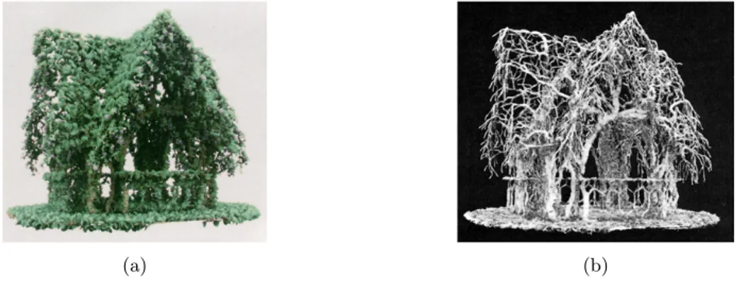
The first method on modeling branching patterns was proposed by Ulam in 1966. The concept was to use cellular automata which had been developed earlier by von Neumann and Ulam [19]. This idea inspired many solutions for plant modeling and was in 1989 extended by Greene [18] to three dimensions and called voxel space automata. It was used to simulate growth processes

that reacted to and sensed the environment. Approaches like this focus on interactions within the growing structure as well as between the environment and the structure, which is a good solution compared to how interactions shape real plants. See Fig.5. A downside is that these methods increase the complexity of the models, and this may be a reason why more simple methods have been influential in plant modeling, even if they ignored issues like collision between branches [19].

(a) (b)

Figure 5: A model from ”Organic Architecture” by Ned Greene, with and without foliage.

The first work in modeling trees in the less complex way began with Honda, who in 1971 proposed a method for modeling trees as recursive branching structures. This idea is the foundation for many generative tree modeling techniques. To view the tree as a recursive branching structure is justified from a biological perspective and the process of tree development [5].

3.6

L-systems

A famous example of a recursive branching technique is the Lindenmayer system (L-system) which was created as a mathematical theory of plant development. The central idea of L-systems is rewriting. Complex objects are described by replacing parts of a simple starting object according to a set of rewriting rules or productions. An example of a graphical object defined by rewriting is the snowflake curve proposed by von Koch in 1904 [19]. See Fig.6.

Figure 6: The Koch snowflake curve[20].

L-systems resemble fractals because of their self-similar nature, but the difference is that fractals are often assumed to exist in an infinite mathematical space and L-system structures are usually limited in their scope and can use various sets of rules on different scales [21].

L-systems are today used in computer games for generating plants and natural environments, but they can also be used in a lot of different applications, for example in pattern design, music composition, modeling of neural networks and arterial branching in medicine [21].

While the L-system with regular patterns of bud distribution and the repetitive character for the potential development, is a good model for young trees and plants, it is not as suitable for mature trees and shrubs [5]. Runions et al. mentions three reasons for this:

1. The fates of the buds are diverse. Some will produce branches or flowers, while some remain dormant or abort. This means that the initial regular bud arrangement will be lost in the older tree.

2. The branches have different fates, some become thick and large, while others remain small or are discarded.

3. The initial branch growth direction will be affected by branch reorientation, tropisms and mechanical bending.

These phenomena have been considered in tree modeling, but most of the techniques still kept the idea of recursive branching, and these factors were seen as modifiers. But in a mature tree, the recursive branching structure is mostly lost and overridden by later developments. In light of this, Runions et. al. proposed a new modeling technique that, instead of using a recursive branching structure, is based on the branches competition for space. The method is based around a space colonization algorithm, and the branching structure of the tree is to large parts decided by the branches competition for space. This method is an extension from an algorithm used to create venation patterns in open leaves [22], [5] and connects to the theories of Ulam and Greene. The environmental factors on plant development is particularly important in complex environments where a number of plants compete for space and light, and to faithfully model a natural growth process that senses and reacts to the environments it is important that the virtual, simulated growth process reacts to and senses the environment [18]. Greene [18] mentions that in crude terms, the environmental factors that affect growth are:

• Available light.

• Obstacles that should be avoided.

• Objects or other organisms in the proximity that promote growth. • Objects or other organisms in the proximity that inhibit growth.

Greene also states that simulated growth processes should at a minimum be aware of these conditions [18].

3.7

Tree modeling with a space colonization algorithm

The main idea when using a space colonization algorithm (SCA) to model trees is to let the tree consist of nodes. New nodes are added through iterations and the placements of new nodes are affected by a set of attraction points that mark available free space. This method makes it possible to generate many different trees and tree-like structures. Another advantage is that the trees and shrubs generated this way adapt to objects or other plants in their vicinity. The foundation for this method is a space colonization algorithm, where competition for space is a key factor deciding the branching of the tree. An advantage of this method is that branch intersections are prevented by the nature of the algorithm.

A recent method for tree modeling with SCA modeled the leaves first and then the branches [23]. They started from a picture of a tree and created a tree crown volume and a color map for the leaves. The branches were then set to grow to fit the tree crown. This is different from previous SCA approaches that started with the branching structure first and created the leaves after the branches. A restriction of this method is that the tree foliage should be dense and that the underlying branching structure is hidden or hardly visible.

Previous implementation Now follows a description of the tree modeling with SCA used by Runions et al. [5].

The process starts with a set of N attraction points and one or more tree nodes. The tree generation is iterative, and in each iteration is it possible for the attraction point to influence the tree node that is closest to it. For a point to influence a tree node, the tree node must be within the point’s radius of influence di. It is possible that many attraction points influence the same

tree node. Runions et al. [5] call this set of attraction points S(v). If S(v) is not empty, a new tree node called v0 is created and attached to node v by a segment (v, v0).

The new tree node, v’, is positioned the distance D from v, and in the direction ˆn. ˆn is defined as the average of the normalized vectors from the tree node towards all the influencing attraction points s ∈ S(v). In formulas: v0_{= Dˆn where ˆn =} −→n k−→n k and − →_{n =} X s∈S(v) s − v ks − vk.

Branching in the tree occurs when a tree node has more than one child tree nodes. Branch weight and tropisms can be simulated by using the equation

˜

n = ˆn+−→g

kˆn+−→g k

where the vector −→g represents the combined effect of tropisms and branch weight which will influence the direction of growth.

After the new tree nodes have been added, the attraction points that should be removed are identified. An attraction point is removed if any of the tree nodes are closer to the point than the kill distance dk.

3.7.1 Parameters influencing the resulting tree shape

To summarize, the parameters mentioned in the algorithm used by Runions et al. [5] are:

Parameter Description

N The number of attraction points

D The distance between a new tree node and its parent.

di Radius of influence, the distance deciding

whether a tree node is affected by an attrac-tion point.

dk Kill distance, the distance deciding if a tree

branch is so close to an attraction point that the point should be removed.

−

→_{g The combined effect of tropisms and branch} weight.

4

Design and technical details

By using sketches of fantasy trees and photos of different and varying tree shapes in nature, a set of parameters was identified. Examples of some tree sketches used can be seen in figure7. To this set was also added the parameters identified from the tree generation algorithm used by Runions et al. [5] displayed in Table1, and some parameters that could extend that algorithm for more variation.

(a) (b) (c)

(d)

Figure 7: Some sketches of trees.

The structure of the implementation was to divide the tree generation into different parts. Attraction points are the points or positions in space that marks the availability of free space. The points can be said to attract the tree branches, and are therefore called attraction points.

The tree branches are represented with tree nodes. If a tree node is inside of the radius of influence of an attraction point, that point may influence the tree node to generate a new point. The uncertainty comes from the fact that in every iteration of the algorithm can an attraction point only influence one tree node at a time. The node-point pair with the shortest distance will decide which tree node the point will influence. The nodes can be influenced by many points in the same iteration, and the resulting direction of the new tree node is based on calculation on the parent node’s set of influencing points.

4.1

Parameters that affect the shape and look of the tree

The set of identified parameters influencing the appearance of the tree is presented in Tables2-5.

Parameter Description

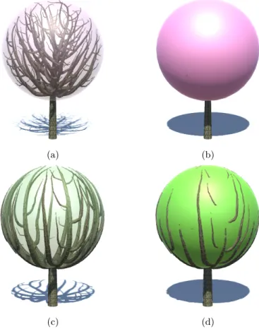
Number of attraction points The amount of attraction points inside a point cloud.

Shape of point cloud The shape and boundaries of the point cloud, for example a sphere and its radius or a cuboid and its width, depth, and height.

Distribution of attraction points inside cloud Where inside the cloud shape are the points positioned? Are they spread out randomly or distributed according to some pattern, for ex-ample only on the surface of the cloud?

Table 2: Point cloud parameters

Parameter Description

Radius of influence If the distance between a tree node and an attraction point is less than or equal to the radius of influence, and that node is the closest node to that point, the point will be part of the set of points that influence the tree node, and affect the position of the nodes child. Kill distance If the distance between a tree node and an

attraction point is less than or equal to the kill distance, that attraction point will be re-moved.

Parameter Description

Segment size The step size, or distance, to how far away from its parent a new node is generated. What would happen if the segment size could vary within the same tree, for example longer seg-ments at the bottom and shorter segseg-ments at the top? Or vice versa.

Branching angle The angle between branches, when a new branch grows from another branch.

Branching factor Can a branching factor be used to control how easily a new branch is created?

Width and circumference The size or volume of the trees trunk and branches, and how it changes with branching. What happens if the pipe model of how branch circumference works in real trees is ignored, and the branch width is decided in another way?

Number of trunks Add multiple trunks to the same tree. They can appear as separate trunks from the ground, or as one trunk that branches into multiple trunks.

Distinction between trunk and branches

Are the trunk (or trunks) to be treated as branches, or should they be separated. Color, material and texture The look of the tree’s surface, for example

bark texture.

Visible roots Are there roots appearing, and how do the roots look.

Gravitational tropism The bending down of branches due to weight and/or gravitation.

Tropism Other kinds of tropism affecting the trees, for example wind.

Light effects Does the tree emit light?

Particle effects Does the tree has some kind of particle effect, for example smoke or fire, coming from it?

Parameter Description

Number of point clouds Add more point clouds, that use different set-tings but interact with the same tree.

Number of iterations The number of iterations and how it should be controlled, for example time, number of points, number of tree nodes, or something else.

Different influence calculations Alternative ways to decide the direction of growth

Varying depth in tree nodes Some branches could have less possible parent-child steps.

Some point clouds only affect some tree nodes

Restrict some points cloud to only parts of the tree, for example a point cloud only affecting the trunk(s).

Make tree nodes attract or repel each other

Add interaction between tree nodes.

Not use closest attraction point in calculation of influencing at-traction point

Use some other calculation to decide which tree node a point will influence.

Influential strength Let the attraction points have different strength and use it to weigh how their influ-ence affects how the branch will grow. Repulsion points Points that will behave the opposite of how

attraction points do, by pushing the tree node away from it.

Layering Can SCA be used to generate a new tree if a branch touches the ground?

Suckering Can SCA be used to generate new tree stems coming from the roots of other trees?

Table 5: Other parameters affecting the appearance of the tree.

4.1.1 Natural growing tree ornaments

There are also things that can grow on trees, like leaves, flowers, fruit, moss, lichen and mushrooms. For each of these the parameters are similar, for example how and where they are positioned on the tree, and their shape and color.

The following are some identified natural growing ornaments that will affect the tree’s appear-ance: • Leaves • Flowers • Fruits • Lichen • Moss • Mushrooms • Other plants

And the following are some parameters that will affect the look of the ornaments and the tree carrying them:

• Positions and distribution • Shape

• Amount

• Color, material and texture • Light effects

• Particle effects

4.2

Selected parameters

Some of the parameters from the presented collection was selected and used in the implementation to add variation to the generated trees. An early choice was to use different kinds of point clouds, referring to groups of attraction points, and to add variation to the points inside the point clouds to see the effects. Due to time restrictions was it not possible to include all the suggested parameters.

4.3

Implementation

An implementation of tree generation with SCA was made in Unity Game Engine and C#. The implementation was a bit different to the algorithm discussed before by the introduction of more parameters. The application consist of a user interface were parameters for the tree can be set, for example segment size. An important part of the implementation is the possibility to add and remove various point clouds. When a new point cloud is added the user can chose its shape, scale and amount of points. After a point cloud is created, it can be selected and moved along the x, y and z-axis in 3D space. The user can add as many point clouds as wanted, and with different settings. The point clouds are treated as one single combined point cloud in the calculations, but where the attraction points can have different radius of influence and kill distance values.

The program can be separated into two parts. The visual parts with user interface, tree, point cloud and scene visualization, and the code parts with the actual algorithms. The visualization and user controls are handled and defined in the Unity Editor. The tree is represented by a Unity game object which has a C#-script connected to it. The script is where the actual SCA tree generation happens.

The C#-script responsible for creating the tree gets the root position from the tree game object, by default set to position (0, 0, 0). The implementation of tree generation with SCA starts by putting a tree node object at the root position. It then loops through all the attraction points comparing them to all tree nodes, to decide where to add new tree nodes. This process is iterative and the algorithm is presented in Algorithm1.

Algorithm 1 The Grow Algorithm

1: if tree node count is 0 then

2: create a new root node

3: add the new root node to the collection of tree nodes 4: end if

5: for all points in the point cloud do

6: for all tree nodes do

7: if distance between point and tree node < point’s radius of influence or tree node is a trunk node then

8: if point have no nearest tree node then

9: set tree node as the point’s nearest tree node

10: end if

11: if distance between point and tree node < distance between point and its nearest tree node then

12: set tree node as the point’s nearest tree node

13: end if

14: end if

15: if distance between point and tree node ≤ point’s kill distance then

16: mark point as reached

17: if point is leaf generating then

18: use random number generation to decide if a leaf should be spawned at tree node position

19: end if

20: end if

21: end for

22: end for

23: for all points in the point cloud do

24: if point has a nearest tree node then

25: add point to its nearest tree node’s set of influencing points

26: reset point’s nearest tree node to null

27: end if

28: end for

29: for all tree nodes do

30: if tree node’s influencing points count > 0 then

31: create a new tree node and add it to a list of new tree nodes

32: clear the tree node’s set of influencing points

33: end if

34: end for

35: for all points in the point cloud do

36: if point is marked as reached then

37: remove point

38: end if

39: end for

40: for all new tree nodes do

41: add tree node to the collection of tree nodes

4.3.1 The user interface

The user interface (UI) was created in the Unity editor, using the built-in Unity UI system. The aim of the UI was to give the user access to as many tree generation settings as possible, while still not take up large screen space. This was achieved by placing all settings in a top and bottom menu, containing sub-menus that can be shown and hidden. See figure 8 for an example where all sub-menus are closed. An example of how it looks when sub-menus are open can be seen in figure9. To move a point cloud it first has to be selected, as can be seen in figure 10. When a new cloud is added it gets assigned a random color and a unique ID. The cloud ID is displayed in the Point cloud sub-menu and the color can be seen on both the point cloud element in the list in the sub-menu and on the point cloud mesh representation. The color was added to increase the usability when building trees of multiple point clouds, since it gives a way to differentiate the clouds just by looking at them.

Figure 8: The user interface. The top menu bar contains from left to right: File (saving and loading), Camera (Rotate camera position), Draw (select tree and point cloud draw mode), Tree (segment size settings, trunk settings, bias vector settings), More (change bark texture), Leaves (leaf settings). The bottom menu bar contains (from left to right): Generate (Different tree generation modes), Randomize (Create a random tree, start and stop randomized auto-generation), Information about number of attraction points, current tree node amount, current number of grow iteration, Move (controls to move point clouds along x-, y- and z-axis), Point cloud (adding and managing point clouds, settings for self-generating point clouds).

Figure 9: Some of the sub-menus are open. The sub-menus can be opened at the same time and will overlap.

Figure 10: The point cloud is selected and can be moved using the move buttons in the Move sub-menu.

4.3.2 Code and scripts

The code used in tree generation is divided between the code for the tree and the code for the point clouds. The tree is created as a SCATree object, containing a set of tree nodes represented as objects of the SCATreeNode class. Each SCATreeNode object has a position and references to its parent and children.

4.3.3 The point clouds

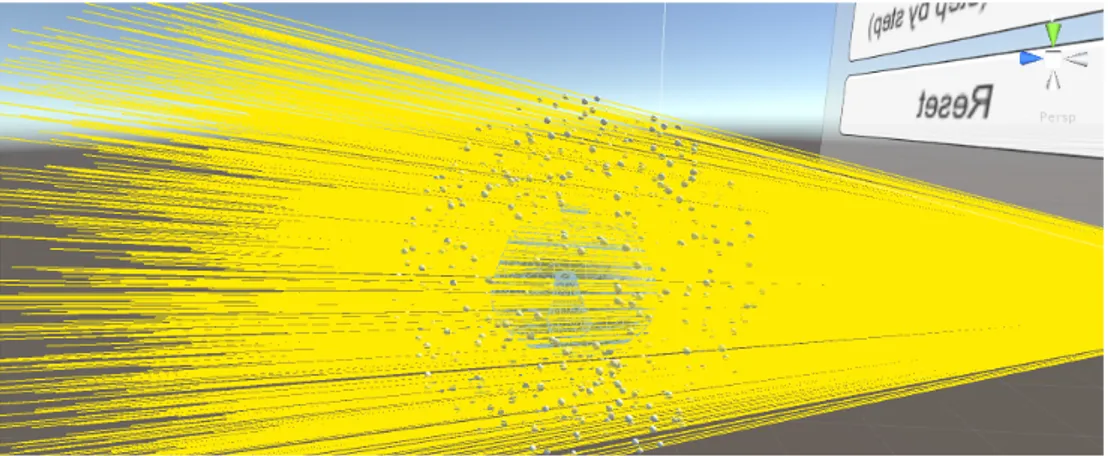
The point cloud class SCAPointCloud is an abstract class from where the different shape-point clouds inherit. There are three point cloud shapes in the implementation: sphere (fig.11), cube (fig.12) and mesh (fig.13). The sphere and the cube, work by randomly distributing points inside or on the surface of a sphere or a cube. The mesh point cloud has a slightly different generation method. It starts by taking the position and the bounds of a mesh that will be used as template for the point cloud. The mesh used in the implementation is the Utah teapot-mesh, see figure13. The application generates a spherical point cloud covering the space of the mesh, see figure14for a visualization example. The rays are cast from the camera towards each of the points, as can be seen visualized in figure 15, counting the number of intersections with the mesh. By doing this for every point, it is possible to find the points contained inside the mesh. The points positioned outside of the mesh are discarded (see fig. 16), and the remaining points are added to a point cloud as attraction points.

(a) (b)

(c) (d)

Figure 11: The sphere point cloud shape. (a) and (b) have a point distribution inside the volume. (c) and (d) have a point distribution only on the surface.

(a) (b)

(c) (d)

Figure 12: The cube point cloud shape. (a) and (b) have a point distribution inside the volume. (c) and (d) have a point distribution only on the surface.

(a) (b)

Figure 14: Visualization of the raycast points generated around the mesh space.

Figure 15: Visualization of the ray casting.

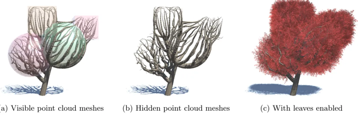
The different point cloud shapes can be combined to create more complex shapes. An example of this can be seen in figure17, where a sphere with points inside the volume, a sphere with points on the surface, a cube with points inside the volume and a cube with points on the surface have been used. When the tree is growing the point clouds are treated as one in the calculations, but they still remain separate which means that they can still be moved or deleted individually.

(a) Visible point cloud meshes (b) Hidden point cloud meshes (c) With leaves enabled

Figure 17: Example of a point cloud composition using spherical and cubical point clouds.

4.4

Tree representation

The actual tree representation that is the final result of the algorithm will be a collection of tree nodes, connected by a parent-child relationship, where each tree node can have zero or multiple children and one parent, with the exception of the root tree node that has no parent. Each tree node has a three dimensional position. This generated tree data is enough for representing the tree, but in the implementation some extra parameters are stored in the tree node object which deals with the three visualization, for example the circumference of the tree in that tree node.

4.4.1 The growth method

The method Grow() is responsible for the tree growth by adding new tree nodes to the tree. The algorithm used in Grow() can be seen as pseudocode in Algorithm 1.

After the actual grow calculations a set of other checks are performed. Depending on which render mode is selected, it is checked if the tree should be visualized with meshes or with simple lines, see figure 18. If the tree is auto-generating some checks are also performed to see if the auto-generation should stop.

(a) Line mode (b) Mesh mode

Addition of a new tree node The new tree nodes are added according to the calculations in the paper [5] from Runions et al. The grow direction deciding the position of the new tree node is the normalized sum of the direction between the parent tree node and its influencing attraction points. If the tree are to be affected by tropism, for example gravity, the bias vector −→g is added to the sum and the new sum is again normalized. The new tree node’s position is calculated as the sum of the parent tree node’s position and the product of the direction vector multiplied by the segment size, D.

4.5

The tree trunk

A problem that occurred when the tree generation algorithm was first implemented was how to deal with the trunk. The algorithm worked when generating the crown, but if the distance between the root position and the point cloud was larger than the points’ radii of influence, a status quo problem occurred where the tree would not start to grow at all, resulting in most of the trees looking more like bushes than trees, because of the need to position the point cloud close enough to the root position. This issue was solved by introducing two categories of tree nodes, trunk nodes and not trunk nodes. The difference is how they are treated in the grow algorithm. The first tree node created is placed at the root position, and will always be set to be a trunk node. As long as the tree has not reached a point cloud, the tree nodes created will be trunk nodes. For a tree node to become a trunk node there are two conditions that have to be satisfied; the tree has not yet reached a point cloud and the new tree node’s parent is a trunk node. The tree is said to have reached a point cloud if the number of deleted attraction points is more than five. The reason for not checking for less, is to better handle cases where there is a large kill distance.

The difference in the grow-algorithm is that when comparing the attraction points to a trunk node, the radius of influence is treated as infinite. That means that for all the points if they do not find any closer tree node, the trunk node will be its closest point. This causes the generation of a tree trunk that grows straight towards the center of the point cloud, since all the points will affect its direction.

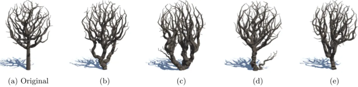
To achieve a more organic look, a randomization setting was introduced, see figure19. If the user selects to use the randomized trunk, the direction vector will be added to a random, direction in space, this is done for every newly added trunk node, and causes a bending, crooked look, compared to the straight trunk.

(a) Original (b) (c) (d) (e)

Figure 19: Example of trunk randomization. Tree (a) is the original tree without trunk ran-domization. Trees (b), (c), (d) and (e) are the same tree as (a) but with trunk randomization enabled.

4.6

Dynamic segment sizes

A new tree setting was introduced where the segment size is randomized between each new run of the algorithm. The range used in the implementation was set to 0.05-0.15. Examples of the result of using the dynamic segment size can be seen in figure20. The use of dynamic segment size result in small variations in the branching of the tree, as can be seen in figure20.

(a) Original (b) (c) (d)

Figure 20: Example of dynamic segment size. Tree (a) is the original tree with a fixed segment size of 0.1. Trees (b), (c) and (d) are the same tree as (a) but with dynamic segment size enabled.

4.7

Bias vector

A bias vector is used to simulate branch weight and tropism, as proposed by Runions et al. [5]. See figure22. Figure22(a) and (b) display the original tree without the influence of a bias vector. A negative x-value causes the tree to be ”pulled” to the left side (fig.22(c) and (d)) and a positive x-value to the right side (fig.22 (e) and (f)). Gravitation can be simulated by using a negative y-value (see fig.22(g) and (h)),which can be compared to the positive y-value (fig.22 (i) and (j)) where the branches grow more straight up. Manipulation of the z-value causes leaning along the z-axis, similar to the effects of manipulating the x-axis. Since the camera used for the example pictures was positioned looking along z-axis, the result of tropism is not as clearly seen as in figure

22(c)-(f). The tree in figure 22 (k) and (l) is leaning towards the camera and the tree in figure

22(m) and (n) is leaning away from the camera. By manipulation of point cloud position and by using tropism is it possible to create smooth, bending shapes, as can be seen in figure21, where (a)-(d) is not using a bias vector compared to (e)-(h) where a bias vector with a negative x-value is used.

(a) (b) (c) (d)

(e) (f) (g) (h)

(a) −→g = (0, 0, 0) (b) −→g = (0, 0, 0)

(c) −→g = (−0.5, 0, 0) (d) −→g = (−0.5, 0, 0) (e) −→g = (0.5, 0, 0) (f) −→g = (0.5, 0, 0)

(g) −→g = (0, −0.5, 0) (h) −→g = (0, −0.5, 0) (i) −→g = (0, 0.5, 0) (j) −→g = (0, 0.5, 0)

(k) −→g = (0, 0, −0.5) (l) −→g = (0, 0, −0.5) (m) −→g = (0, 0, 0.5) (n) −→g = (0, 0, 0.5)

To get even more variation a bias vector with more than one nonzero component can be used, with some examples displayed in figure23.

(a) −→g = (−0.5, −0.5, −0.5) (b) −→g = (−0.5, −0.5, −0.5)

(c) −→g = (0.5, 0.5, 0.5) (d) −→g = (0.5, 0.5, 0.5)

(e) −→g = (−0.5, 0.5, 0) (f) −→g = (−0.5, 0.5, 0)

(g) −→g = (0.5, −0.5, 0) (h) −→g = (0.5, −0.5, 0)

4.8

Dynamic bias vector

A new feature that was added was the use of a dynamic bias vector. That means that the bias vector changes after some iteration steps. When manually building trees the bias vector changes to a random vector after 10 iteration steps. When using randomized trees also the iteration step value is randomized. Some examples of trees generated with a dynamic bias vector can be seen in figure24. Those trees were created manually, which means that they were assigned a new, random bias vector every 10th iteration step.

(a) (b) (c)

Figure 24: Trees generated with dynamic bias vectors.

By using the dynamic bias vector together with randomized trunk and dynamic segment size, some more various trees can be generated as can be seen in figure25.

(a) (b) (c)

(d) (e) (f)

Figure 25: Trees generated with randomized trunks, dynamic segment sizes and dynamic bias vectors.

4.9

Leaves

The tree application has a set of 13 leaf types. A random leaf type from that set is chosen when using the randomization feature. The color is also set by the user or randomized, including the transparency of the leaf. When a tree node causes an attraction point to be deleted, there is a random chance for that tree node to spawn one or more leaves in its position. The probability to spawn leaves is also randomized when using the randomization feature. The number of leaves spawned in each leaf position can also be set by the user, or be randomized.

4.10

The tree mesh

The trees are covered in bark material. The tree application has a set of 15 different selectable bark textures, and one is randomly selected when randomizing a tree. The tree is not a single mesh, but are using Unity prefabs. A prefab in Unity is an object that acts as a template and can be instantiated [24]. Each tree segment is rendered with a cylinder prefab that is instantiated positioned between every tree node pair and rotated based on the rotation between the tree node parent-child pair. The cylinder’s height is scaled to match the distance between the points (the segment size) and its radius is scaled according to the trees trunk and branch circumference. An issue with this solution is that it sometimes creates gaps in the branches, in the joint between two branch segments, see figure26.

4.11

Auto-randomization and -generation

After the user controls for building trees were in place, a process began to let the application randomize the settings and auto-generate and automatically save trees. The purpose of this was to investigate the possibilities to generate a wide variety of trees. The application now have a start and a stop button. When start is clicked, the application starts to generate random trees and saves them until it is stopped. The trees are saved in three file formats: a screen shot of the generated tree, a text file with information about the tree and a .treedata file, that can be used to load the tree parameters back into the application. The data stored in the .treedata file is not the actual tree nodes and attraction points, but the parameters used for generating the point clouds and the tree. The result of this is that the loaded tree will not always look exactly like the previous tree, but it will have the same features, and by that look like it belongs to the same species of trees.

4.12

Self-generating point clouds

The application contains two types of tree randomization. The first tree randomization solution generates a random number of point clouds before the tree node generation starts. The second solution creates new point clouds during the tree node generation, called self-generating point clouds. When using the self-generating point clouds is the Grow()-method extended, so that a check is performed at the start of the algorithm to see if there exists any point clouds. If no, a point cloud is randomly generated. The tree continue to grow and when it reaches the point where the tree generation would stop, a new point cloud is added and the tree growth continues. This goes on as long as the maximum number of point clouds is not reached, at which point the tree generation finish. When using randomized trees the maximum number of point clouds is also randomized. There are two modes for how the point clouds are created. The point clouds can either be randomized individually or use inheritance so that the first point cloud will be randomized and the rest will use the same settings as the first point cloud when they spawn.

5

Results

Here follows some examples of trees generated with the implementation. A number of sessions of tree auto-generation where performed and some of the resulting trees are presented here. The purpose of the auto-generation was to explore the range of tree variation supported by the imple-mentation.

5.1

Manually constructed trees

Here are some trees that were user constructed by manually creating point clouds, positioning them and adjusting the settings of tree growth. It is possible to create more complex shapes by combining the basic point cloud shapes. An example of this can be seen in figure27. The spheres were position in a conical shape, with some smaller sphere positioned in the middle and up. The small spheres where created with a stronger radius of influence than the larger spheres. The reason for this was to pull the tree towards the small spheres, to try to create the look of a spruce-like tree. The tree depicted in figure27(a), (b) and (c) use a bias vector −→g = (0, −0.01480466, 0) and the tree in figure27(d), (e) and (f) use a bias vector −→g = (0, −0.5, 0) to simulate a stronger force down. The trees are otherwise identical in settings.

(a) (b) (c)

(d) (e) (f)

Another example of creating shapes with point cloud combinations can be seen in figure 28

where 15 spherical point clouds with the same settings are positioned in the shape of heart.

(a) (b) (c) (d)

Figure 28: Example of building a heart shape using spherical point clouds.

5.2

Randomized and auto-generated trees

Some trees were generated with a random initial distribution of point clouds and some with point clouds added dynamically during the tree growth. The trees in figures30-33were generated with having all point clouds randomly spawned at the start.

Sometimes the tree randomization resulted in more realistic or ”normal” trees, see figure29.

(a) (b)

Figure 29: ”Normal” looking trees. (a) is generated with all point clouds from the start and (b) is generated with self-generating point clouds.

The features of the trees showed large variation within the scope of the randomization limits. An example is the branch circumference, as can be seen in figure30. These trees where generated immediately after each other and displays how the appearance of the tree changes with the trunk and branch circumference.

Some trees got curving branches (see Fig. 31(a)) while others had a more spike-like straight appearance (see Fig. 31(c)). In some trees was it very clear which point cloud shape that was used, like in figure31(b) where a spherical point cloud has caused the branches into a cage-like look. Some trees grew low and along the ground, like figure31(c) and (d), resembling the look of a krummholz tree.

(a) (b)

Figure 30: Examples showing thickness variation.

(a) Squiggly branches (b) A distinct spherical branch shape

(c) A ground growing tree (d) Ground crawling

Some of the generating trees could be said to challenge the border between plant and creature, for example the trees in figure32and 33. The look of some trees could be called ”monster”-like and creature-like, with the look of claws grasping in the air or with crawling snake-like parts.

(a) (b)

Figure 32: Randomized trees

(a) (b)

Figure 33: More randomized trees

To show the variation a set of trees auto-generated with leaves are displayed in figure34and some trees generated without leaves in35. There are various trees in both groups, and as can be seen is it not only the leaf shape and color that influence the appearance of the trees, even if it has a big impact on making the trees look more imaginative.

(a) (b) (c) (d)

(e) (f) (g) (h)

(i) (j) (k) (l)

(m) (n) (o) (p)

(q) (r) (s) (t)

(a) (b) (c)

(d) (e) (f)

(g) (h) (i)

(j) (k) (l)

(m) (n) (o)

Figure 35: Randomized trees without leaves made with point clouds added at the start of the generation.

Self-generating point clouds The trees in figure36are some examples of trees generated with point clouds added automatically during their growth, which exemplifies a shorter type of trees compared to the trees in figure38that also features trees made with self-generating point clouds.

(a) A short and fluffy tree (b) Tree with a squiggly trunk

Figure 36: Trees made with self-generating point clouds

The self-generating point clouds can also result in trees with a ”tropism look”. The tree in37

is an example of this. The branches of the tree are positioned on one side of the tree, causing a look that is similar to trees affected by for example strong winds.

Figure 37: Self-generated point clouds causing a tropism look

A feature seen in some of the trees created with self-generating point clouds is a type of spikes coming out as short branches from the trees’ branches, as can be seen in figure38.

(a) (b) (c)

(d) (e) (f)

Figure 38: Trees made with self-generating point clouds

5.3

Generation time

To evaluate how fast a finished tree could be generated a timer was added to measure the generation times of the trees. The generation times in milliseconds for the trees in figure35 are presented in the bar chart in figure39, and the generation times for the trees in figure38 are presented in the bar chart in figure40. The trees where generated on a computer running Windows 7 64-bit operating system, Intel Core i7-5960 CPU and RAM 16 GB. An interesting thing to notice is that the generation times for the trees using self-generating point clouds in figure38are quite fast compared to the trees in figure35, even though the trees in figure38look bigger and have leaves. A reason for this may be that since they are using self-generating point clouds are the point amount from the start not as large.

Figure 39: Generation times for the trees in Fig. 35.

Figure 40: Generation times for the trees in Fig. 38.

5.4

Iteration time

To evaluate the performance of the grow algorithm (Algorithm1) a set of trees where generated with the time measured for each iteration. The number of tree nodes increases and the number of attraction points decreases during the tree generation. There was a perceived spike where the generation felt like it was going slower the more the tree grew, and that it sped up at the end. To investigate this, a timer was added to the grow algorithm and used for measuring each iteration in milliseconds. The result is presented in figure41. The grow iteration tests were performed on a laptop running Windows 10 64 bit operating system, Intel U7300 CPU and RAM 4.0 GB. The trees used were randomized and created using the auto-generation and randomization feature in

the application, and are presented in figure42.

Figure 41: A line graph displaying the render times in milliseconds for each iteration of 9 trees.

The result of the test that is presented in the graph in figure 41 indicates that there is an increase in grow-iteration time, up to a certain point where it becomes shorter again. This pattern can be seen in most of the generated trees, with some examples having a more steep time curve, like Tree 3, 5, 6, 8 and 9. Some of the trees’ data is presented in Table6.

Tree Generation time (ms) Total grow iteration time (ms) %

Tree 1 326 36 11 % Tree 2 4471 3773 84 % Tree 3 8684 7682 88 % Tree 4 1343 960 72 % Tree 5 4560 4106 90 % Tree 6 22438 21453 96 % Tree 7 5694 4918 74 % Tree 8 5582 4814 86 % Tree 9 2230 1735 78 %

Table 6: Data for the trees used for time measuring. The last column displays the percentage of generation time spent on the grow algorithm.

As can be seen in Table 6 was a majority of the tree generation time in most cases spent on the grow algorithm.

(a) Tree 1 (b) Tree 2 (c) Tree 3

(d) Tree 4 (e) Tree 5 (f) Tree 6

(g) Tree 7 (h) Tree 8 (i) Tree 9

6

Discussion

The idea of the implementation is to give the user tools to build tree-like structures with three-dimensional point clouds as building blocks. Based on the point cloud setting, the different cloud blocks get varying amounts of attraction points, different point distributions, radius of influence and kill distance for the points inside the point cloud. The idea of this implementation was to increase the amount of parameters affecting the resulting tree shape to increase variation. Many types of trees and tree-like structures can be built by using various point clouds with different settings. Some of the new parameters introduced in this thesis is the trunk node, the randomized trunk node, the dynamic segment size, the dynamic bias vector, the randomized point clouds and the self-generating point clouds. These factors contribute to the range of variation seen in the resulting trees.

The resulting trees will vary in the randomized range. It is possible that larger variations could occur if the range was increased. The range chosen in this implementation was selected to minimize the number of cases where tree generation stops before there is a tree shape at all. Still, as presented in the results, these cases did happen, and even though there were multiple point clouds, the tree did not manage to grow far up before reaching a halt. A solution to the problem with halting tree growth could be to use the dynamically added point clouds. If the tree growth stops a new point cloud would be added in a way that ensures that it will affect the tree growth, and that the tree growth will not stop prematurely.

Something that could be seen as both a problem and a feature is the trunk spikes that occurred during the use of self-generating point clouds. A possible solution to avoid these spikes would be to limit the effect of the new point cloud to only the most recently added tree nodes.

The leaves gives the tree its character. The leaf shape, color and positioning has a big impact on the appearance of the tree, and the variation could be even larger if more tree ornaments, for example mushrooms or flowers, were added. A feature of the leaves that was not parameterized was the rotation, a way to add more variation would also be to make different kinds of leaf rotation possible. In the current solution is the leaves rotated in a random direction. But even if the leaves are disregarded is the current solution able to generate a wide range of different tree structures.

The implemented SCA tree generation could be seen as tool, material or designer according the four views on PCG systems proposed by Khaled et al. [7_{]. The tool metaphor means that}

the designer gets increased capabilities, and it applies since the application makes it possible to generate complex tree structured with ease. The calculation used for determining the branch direction would for example be very time consuming if made manually. The material metaphor describe how the procedural content act as a new material for the designer to work with. This is also true for tree generation with SCA. The process of adding and organizing different point clouds to guide the growth of a tree, can be seen as new material. The designer is not manipulating the actual tree, but instead the space where the tree can grow. By adjusting parameters of the tree, for example segment size, is it possible for the designer to also describe how the tree grows. Earlier works [18] on tree and plant modeling have stated that it is important that the virtual, simulated growth process reacts to and senses the environment if we want to faithfully model a natural growth process that senses and reacts to the environment. The implemented tree generation has this in parts, since the point cloud composition defines the external factors, and tree parameters like segment size, can represent the tree’s internal factors, and it could be further extended to allow for more environmental influence, for example by letting light and shadow affect the generated point clouds. This solution can also be said to satisfy the conditions of the designer metaphor of Khaled et al. [7]. The randomization feature can be used to generate a wide variety of trees and tree-like structures. The designer can use the auto-generation features to fast get a large set of different trees, and then go through them to select the preferred ones. By using the save files is it also possible to open the tree data and adjust it as wanted.

Now follows a discussion of the solution related to the taxonomy of PCG proposed by Togelius et al. [4] and Shaker et al. [8].

Online or offline The current tree generation implementation is to slow to immediately generate a full grown tree, so it would be more suitable for offline generation, for example generating the trees just before the start of a game session. However, the current trees can be used in for

online generation also. The tree can be set to render in each iteration, causing a visible growth process. If it is preferable to see the growing process this solution can be used for that.

Necessary or optional The generated trees would probably be more suitable for the optional game content category. Because of the random elements is it not always clear how the final tree will look. If the trees are just used for decoration purpose it would be suitable to define them as optional content.

Generic or adaptive The trees could be made both generic or adaptive, i. e. adapt to player behavior or not. If the trees would get information about the player it could parameterize it and use it in the tree generation. For example generate larger or more dense trees if the player moves slower, or use a bias vector directed at the player position.

Stochastic or deterministic The implementation can be both stochastic and deterministic, it depends on which settings are used. If the randomized trunk, dynamic segment size or the dynamic bias vector is used is it stochastic. But if not will the tree be regenerated the same every time. Since the save is not storing the points, but the point cloud parameters, will the saved tree and the loaded tree not be identical, even if none of the randomization settings are used. Thus, is the solution more suitable for stochastic modeling.

Constructive or generate-and-test The current solution is constructive, it generates the content once and will not process it more after that. It would however be possible to make it generate-and-test. A suitable extension would be to test if the generated tree reached all point clouds. This is not tested in the current solution, and it can result in trees not growing as the designer intended, if the distance between point clouds is too big.

Automatic generation or mixed authorship The implementation supports automatic generation since the designer is specifying the parameters of the tree and its environment, letting the algorithm handle the content creation. It could be possible to make it as mixed authorship if the designer could model parts of the tree and then use the algorithm to finish it. For example could the designer draw the trunk, and then be enabled to move the root position to decided where to start the algorithmic tree generation from.