f-G+ lel l ms! <F iB. <F " Tads =-" ke Saws Optimisation of single horizontal curves in railway alignments Bjorn Kufver
i I<FB
Swedish National Road and
some.""
jTransport Research Institute
VTI rapport 424A- 1997
Optimisation of single
horizontal curves in
railway alignments
Bjorn Kufver
1
.
SWMMP mm: mggm
ansptm
instimo
IZTH
Cover: VTI
CCCCCCCCCCCCC NS RRRRRRRRRRR RD
Publisher: Publication
VTI Rapport 424A
Published Project code
Swedish National Roadand 1997 70041
' anspart Research Institute
Project
Optimisation of track geometry
Author Sponsor
Bj ('jrn Kufver Adtranz Sweden, Swedish National Rail Administration
(BV), Swedish State Railways (SJ), Swedish Transport and Communications Research Board (KFB) and Swedish National Road and Transport Research
institute (VTJ)
Title
Optmisation of single horizontal curves in railway alignments
Abstract
This report describes procedures for optimisation of the alignment of single curves. The effects of using passenger comfort on curve transitions (PCT) as an object function are quanti ed. Both the choice of cant and the choice of lengths of transition curves are analysed.
Comprehensive vehicle and track models for dynamic analysis are presented. A Euro ma standard coach (UIC-Zl) represents a conventional vehicle with a roll coef cient of 0.2 (effective roll factor 1.2) and an SJ UA2 coach represents a tilting coach with an effective roll factor (the total effect of the roll coef cient and the active tilting) of approximately 0.3. An SJ X2 power car represents a suitable high speed locomotive for tilting as well as non-tilting coaches.
Dynamic PCT analysis is conducted on certain alignment alternatives. An evaluation of other vehicle reactions, such as wheel/track forces and climbing ratios provides no formal reason for excluding any of the alignment alternatives, except when the power car is running on cant de ciencies exceeding 415 mm. However, these exceptional cases are of no practical interest since the corresponding PCT values are in any case non-optimal.
The in uence oftrack irregularities on the optimal solutions has not yet been investigated.
The optimal lengths of the transition curves depend mainly on the roll coef cient of the vehicle, a possible body tilt system, the change in direction between the adjacent straight lines, and the positions of the binding obstacles.
The optimisation with the procedures in this report leads to alignments which are better prepared for future traf c demands, without signi cantly increased construction costs.
ISSN: Language: No. of pages:
Preface
This work has been carried out at the Division of Railway Technology, Department of
Vehicle Engineering, Royal Institute of Technology (KTH), Stockholm and the Railway Systems Group, Division of Transport Systems, Swedish National Road and Transport Research Institute (VTI), Linkoping.
The work is part of the joint project concerning track/vehicle interaction commissioned by Adtranz Sweden, the Swedish National Rail Administration (Banverket), the Swedish Transport and Communications Research Board (KFB), the National Swedish Board for Technical and Industrial Development (NUTEK), the Swedish State Railways (SJ), and the Swedish National Road and Transport Research Institute (VTI).
The nancial support provided by Adtranz Sweden, Banverket, KFB, SJ, and VTI for the present work is gratefully acknowledged.
A model of the Euro ma standard coach has been provided by DEsolver AB and models of the SJ X2 power car and SJ UA2 tilting coach have been provided by Adtranz Sweden. Special thanks are due to Ingemar Persson, DEsolver AB, Nils Nilstam,
Adtranz Sweden and Lars Ohlsson, Adtranz Sweden.
I would also like to thank Professor Evert Andersson at KTH for his support during the
course of the work.
Linkoping, October 1997
Cover illustration: The Southern Main Line (left) and Western Main Line (right) in Katrineholm. The diamond crossing constitutes a (non-binding) longitudinal obstacle for the superelevation ramp on the Southern Main Line, since cant is not permitted in obtuse crossings in Sweden. Also the contrary flexure turnout on the up line of the Southern Main Line constitutes a (non-binding) obstacle, since the cant excess in the branch line must be limited
KTH TRITA-FKT Report 1997:45
VTI Rapport 424A
KTH TRITA-FKT Report 1997:45
VTI Rapport 424A
TABLE OF CONTENTS
Summary
1. Introduction
1.1 Objective of the present research project
1.2 Object functions and boundary conditions for optimisation 2. The use of present track geometry standards
2.1 The choice of cant
2.2 The choice of horizontal alignment 3. Simplified analysis of passenger comfort
3.1 PCT as a function of track quantities, vehicle speed and effective roll factor
3.2 PCT and the choice ofcant
3.3 PCT and the choice of horizontal alignment 4. Models for dynamic track/vehicle analysis
4.1 GENSYS multibody computer code
4.2 Model of the Euro ma standard coach UlC-Zl 4.3 Model of the SJ UA2 tilting coach
4.4 Model of the SJ X2 power car 4.5 Track model
5. Dynamic analysis of alignments without track irregularities 5.1 Vehicle reactions on linear superelevation ramps 5.2 Vehicle reactions on curves without track irregularities
5.2.1 Initial study of the dynamic PCT evaluation
5.2.2 Conventional coach on curves without track irregularities 5.2.3 Tilting coach on curves without track irregularities 5.2.4 Power car on curves without track irregularities 5.2.5 Discussion of the results from the dynamic analysis
6. Conclusions References
Appendix 1 Terminology and definitions Appendix 2 Notations
Appendix 3 Certain mathematical expressions concerning track quantities
Appendix 4 Variables and limit values for evaluation of railway alignments
Appendix 5 Radii and cant deficiencies on the curves studied Appendix 6 Wear indices, low frequency lateral acceleration and
low frequency lateral jerk in the dynamic analysis
KTH TRITA-FKT Report 1997:45 VTI Rapport 424A
O O U J U J r d r I l 13 l3 16 26 33 33 35 38 4O 41 42 42 46 46 50 54 58 62 63 65
KTH TRITA-FKT Report 1997145 VTI Rapport 424A
Summary
This report describes procedures for optimisation of the alignment of single curves. Chapter 2 describes a number ofrelevant limits in the Swedish track geometry standards and shows how cant may be chosen in predetermined alignments when permissible
speed is to be maximised. The chapter also shows how the alignment may be designed
when taking obstacles into account and the permissible speed is to be maximised.
The effects of using passenger comfort on curve transitions (PCT) as an object function are studied in Chapter 3. Again, the choice of cant is analysed rst and thereafter the choice of lengths of transition curves is studied. The vehicle reactions are Simpli ed and translational accelerations caused by rotational velocities and rotational accelerations are ignored.
In Chapter 4, the vehicle and track models in the dynamic analysis are presented. A Euro ma standard coach (UlC-Zl) with FIAT bogies (0270) represents a conventional vehicle with a roll coef cient of 0.2 (effective roll factor 1.2) and an SJ UA2 coach
represents a tilting coach with an effective roll factor (the total effect of the roll
coef cient and the active tilting) of approximately 0.3. An SJ X2 power car represents a suitable high speed locomotive for tilting as well as non-tilting coaches.
Dynamic vehicle reactions on track geometries without track irregularities are studied in Chapter 5. Firstly, vehicle reactions on strictly linear as well as smoothed superelevation ramps are evaluated. It is concluded that the superelevation ramps may be assumed to be strictly linear in this study, even though they may be slightly smoothed in reality. It is also concluded that it is more favourable to arrange the superelevation ramp by twisting the track around its centre line compared to twisting the track around its inner rail. Secondly, dynamic PCT analysis is conducted on some of the alignment alternatives
presented in Chapter 3. An evaluation of other vehicle reactions, such as wheel/track
forces and climbing ratios provides no formal reason for excluding any of the alignment alternatives, except when the power car is running on cant de ciencies exceeding 415 mm. However, these exceptional cases are of no practical interest since the corresponding PCT values are in any case non-optimal.
The in uence of track irregularities on the optimal solutions has not yet been investigated.
The optimal lengths of the transition curves depend mainly on the roll coef cient of the vehicle, a possible body tilt system, the change in direction between the adjacent straight lines, and the positions of the binding obstacles.
The optimisation with the procedures in this report leads to alignments which are better prepared for future traf c demands, without signi cantly increased construction costs. If the optimisations lead to alignments where potential permissible speed varies greatly between different single curves, the number of curves which may have to be realigned in the future (and the associated future construction cost) will be reduced.
KTH TRITA-FKT Report 1997245 i
Keywords: Vehicle dynamics, simulation, track/vehicle interaction, track geometry, cant, alignment, transition curve, wheel force, guiding force, track shift force, climbing
ratio, wear index, passenger comfort, PCT.
ii KTH TRITA-FKT Report 1997:45
1.
Introduction
1.1
Objective of the present research project
Railway alignment has a high degree of permanence. When the alignment is altered, several technical subsystems, such as substructure, superstructure, catenary systems, etc., must be altered as well. Therefore, changes in the alignment are normally associated with high costs. This indicates that while the alignment of new railways should be designed to meet future traf c demands, an unnecessarily high standard may make a project too expensive and may cause undesirable impacts on the environment. These facts lead to the conclusion that the alignment should be optimised with great care when building new lines.
The objective of the present report is to develop methods of optimising the alignment when building new lines and renewing existing ones.
1.2
Object functions and boundary conditions for optimisation
The ideal objective function when optimising alignments should consider all relevant
aspects, such as construction costs, maintenance costs, costs of train operation and
generalised costs representing time costs, discomfort for passengers, undesirable impacts on the environment, etc.
Mathematical methods for calculation of the optimal highway location have been presented by Nilsson (1982) as well as others. In his approach, Nilsson used established
cost functions concerning capital, road construction, road maintenance, road operation,
road accidents, vehicle use, generalised time costs and generalised costs related to traf c
noise.
In railway engineering, there is a lack of knowledge concerning some of the cost functions. Contrary to road engineering, accident costs are very low since accidents are rare. Another difference is that vehicle speeds are higher on railways than on highways with similar alignments. On a Swedish highway with a design speed of 110 km/h, the minimum radius is 600 metres, being derived from limits based on friction between tyres and road, but usually limits for sight distances require larger radii (V'agverket 1994). On railways with modern tracks (continuously welded rails, heavy sleepers and high quality fastenings), permissible train speeds are to a great extent related to ride comfort on horizontal curves. On a circular curve of 600 metres radius, the permissible train speeds are in the range 110-140 km/h, if cant and adjacent transition curves are properly arranged (according to the limit values of Banverket 1996). Hence, it is important to consider passenger comfort related to translational and rotational motions, especially since train passengers are free to stand and walk around in
the trains.
Passenger comfort on curve transitions, PCT, is an index which relates lateral jerks, lateral accelerations and roll velocities to the percentage of passengers who are
dissatis ed with the comfort (CEN 1995, Eickhoff 1997, Harborough 1984, 1986, ORE
KTH TRITA-FKT Report 1997 :45 l VTI Rapport 424A
1987). It has been concluded that the PCT functions are the most reasonable functions for evaluation of discomfort primarily due to the alignment and cant, since the physical quantities which are evaluated are related to curve radii, lengths of transition curves and cant (Kufver 1997b). It should be noted that none of the cost functions used by Nilsson (1982) considers the lengths of transition curves.
However, since PCT is expressed in non-monetary units, it will be used in this study as
an object function for comparing alignment alternatives with equalconstruction costs. The study will consider the most frequent case in a design process; a clothoid circle -clothoid combination between two straight lines, and an approach presented by Kufver (1997a) will be used to de ne the equally costly alignments. According to this approach, differences in construction costs depend mainly on the extent to which existing obstacles along the alignment must be removed or dealt with alternative measures. At another level of optimisation, it may be interesting to compare the alignment alternatives associated with different construction costs. In such an analysis, it seems reasonable to compare the best alignment alternative at each cost level, derived with the methods in this report.
Other aspects of track/vehicle interaction, related to safety, wear and maintenance, such as vertical and horizontal forces on the track, climbing ratios and wear index, are calculated through simulation, and are monitored and sometimes used in boundary conditions according to procedures presented by Kufver (1997c). Most of these procedures are the same as in CEN TC256 WGlO (1996) and UIC 518 OR (1997) with some minor changes. If the alignments to be evaluated are located on a freight only line, it seems more reasonable to use one or a combination of the variables related to safety, wear and maintenance as an object function (Kufver 1997c). A summary of the criteria is presented in Appendix 4.
PCT has been used in the evaluation of passenger comfort resulting from the track/vehicle interaction by Hohnecker (1993), Pospischil (1991) and UIC (1991), but in none of these studies was it used as an object function and none of the studies considered the dynamic behaviour ofthe vehicle.
In Chapter 2, procedures for optimisation alignment and cant, considering present track geometry standards, are developed. By comparing the optimal solutions in Chapter 2 with the optimal solutions from the optimisation considering track/vehicle interaction, we may evaluate whether or not the track geometry standards provide resonable guidance for track engineers.
In summary, passenger comfort will be used as the object function in this report. Construction costs and other aspects of track/vehicle interaction will be treated in boundary conditions.
2 KTH TRITA-FKT Report 1997145 VTI Rapport 424A
2.
The use of present track geometry standards
2.1 The choice of cant
Swedish limits for a number oftrack geometry quantities are shown in Table2. l. Maximum cant 150 mm
Maximum cant de ciency 100 mm Maximum cant excess 100 mm Maximum cant gradient 1:400 Maximum rate of cant 46 mm/s Maximum rate of cant de ciency 46 mm/s
Table 2.] Swedish limitsfor a number oftrack geometry quantities, applicable to conventional vehicles, class A. (Source: Banverket I996)
The limits1 are applicable to class A vehicles. After special investigation, vehicles may
be classi ed differently, and allocated other limits for cant de ciency, rate of cant and rate of cant de ciency.
In the literature, it is reported that railways in other countries use basically the same kind of limits. Exceptions are the rules reported by Loach and Maycock (1952) where the limit for cant de ciency was reduced by increasing cant, and older Swedish track geometry standards where the limit for rate of cant was reduced if the cant was lower than a normal value of the cant, which was two thirds of the equilibrium cant (SJ 1978). In Germany and France, the limit for cant excess depends on the traf c load of slow trains (Weigend 1982). Since 1996, the Swedish limit for cant excess is lower (70 mm) if the curve radius is smaller than or equal to 1000 m (Banverket 1996). However, no indication was given concerning the freight train speeds for which the cant excess should be calculated.
In the 3-dimensional case where cant de ciency, rate of cant de ciency and rate of cant are studied, the present Swedish track geometry standards may be illustrated as a rectangular box. A combination where these quantities are slightly below their limits (point A in Figure 2.1) is permissible, but a combination where one of the quantities is slightly above its limit (point B) is not permissible, irrespective of the margins for the limits of the other two quantities.
1 There are exceptions for these limits. For example, the limit for cant de ciency is lower in some turnouts and no cant at all is allowed at obtuse crossings.
KTH TRITA-FKT Report 1997:45 3 VTI Rapport 424A
Limits of cant de ciency, rate of cant and rate of cant de ciency
Cant deficiency T
A
,1» --- --- ---- -- / > Rate of cant u - n $ u - -
.-l . . . - - u u - . . n . . . .I
5/Rate of cant deficiency
Figure 2.1 A permissible (A) and a non-permissible (B) combination of cant de ciency, rate of cant de ciency and rate ofcant according to present track geometry standards.
The limits in Table 2.1 often give the track engineer some degree of freedom in choosing a suitable cant. In Sweden, additional guidance for the choice of cant is given in a handbook (Banverket 1996). This includes the following recommendations: cant should normally be two thirds of equilibrium cant and cant de ciency for conventional passenger trains should be of the same magnitude as cant excess for the slowest freight trains. However, these rules are normally not compatible with each other.
Other guidance is given by other railway companies. According to BL. Cope (1993) it is advisable to use a cant such that cant and cant de ciency are about the same. Hence, the cant should be 50% of the equilibrium cant. Swiss Federal Railways (SBB 1969) stated that a normal cant is 55% of the equilibrium cant (if the maximum permissible speed on the curve is not higher than 125 km/h). German Federal Railways (DB) use a normal cant which is 60% of the equilibrium cant, but if all the trains have the same speed the cant may be 100% of equilibrium cant (Weigend 1983). The French State Railways (SNCF) use empirical rules which result in a cant equal to 65-79% of the equilibrium cant (Alias 1984).
Various other principles have beenused in Russia and Belgium. According to Kohler (1980), the Russian railways design the equilibrium cant for a weighted speed (Vw), which is calculated as the root of the average of the squared train speeds, and where the weights (mi) equal the tonnage of the trains at each level of the train speed, see equation [2.1]. In this way, the sum ofthe products oftonnage and cant de ciency will be zero.
4 KTH TRITA-FKT Report 1997:45 VTI Rapport 424A
[2.1]
On high speed lines in Belgium, the normal cant corresponds to 50 mm of cant de ciency (Raviart 1996).
In Sweden, there has been great interest during the last 10 years in increasing the permissible speed on existing lines, for conventional train as well as for tilting trains. Two questions then arise: How can permissible speed be increased by a change of cant alone and how can permissible speed be increased by a change in the horizontal alignment as well as the cant?
The rst question may be answered by illustrating the limits in Table 2.1 in a diagram. The following gures show the permissible cant as a function of the permissible speed for a circular curve with a radius of 2000 m and transition lengths (clothoid lengths) of 70 m, 130 m and 190 m respectively. The speed of slow freight trains is restricted to 90 km/h.
200
I I
- \ / / Minimum cant -"H-'4":::::::::::::::::::::i::::::4::::':::::: :0 150 ________ = 150 mm ' // -- Cant excess A // = 100 mm E _ ,/E, 100 _____,x
- Cant de ciency
*5 = 100 mm 8 _ Rate of cant _ Permissible zone = 46 mm/S50 -- a Rate of cant de ciency
- = 46 rnm/s
mum Cant gradient ' = 1/400 0 I l l l l ' ' ' l | l l " V l l 1 ' V l I 1 ' l l
0 50 100 150 200 250
v (km/h)
Figure 2.2 Permissible cant on a curve with veryshort clothoid lengths.
KTH TRITA-FKT Report 1997:45 5
200 ' - Minimum cant = O ' , Maximum cant 150 _ //x __________________ " = 150 mm // A , x - Cant excess
5
-
= 100 mm
:: 100
-5 - o Cant de ciency O Permissible zone = 100 mm Rate of cant50 "
= 46 mm/s
a Rate of cant de ciency
_ = 46 mm/s O I I I I l I I I I l I I I ' I I I I I I I
O 50 100 1 50 200 250
v (km/h)
Figure 2.3 Permissible cant on a curve with short clothoid lengths.
200
' Minimum cant = O150
//,"""""""""
= 150 mm
// , / Cant excess = 100 mm I a + Cant de ciency Ca nt (m m)ES
0 Permissible zone = 100 mm Rate of cent50 "
= 46 mm/s
+ Rate of cant de ciency
_ = 46 mm/s
O I I I I i I I I I i I I I' I i I I - I I i l l l I
0 50 100 150 200 250 V (km/h)
Figure 2.4 Permissible cant on a curve with long clothoid lengths.
On a curve with very short transition curves, the limits for the rate of cant and the rate of cant de ciency constitute binding constraints. If the transition curves are short (but not
6 KTH TRITA-FKT Report 1997 :45 VTI Rapport 424A
very short), the limits for cant de ciency and the rate of cant are binding. If the conditions in the transition are not binding, the transition curves may be de ned as long. In this latter case, the permissible cant de ciency and either the permissible cant or the permissible cant excess for slow trains will be binding.
If track engineers seek to maximise the permissible speed in existing alignments, they will choose a cant as far to the right as permitted in the gures above. The question for the researcher and the author of the track geometry standards is whether or not these
solutions represent the most suitable cant according to the interaction between vehicles
and track. (It may be noticed that the cant which maximises the permissible speed, according to Swedish limits, is not a xed proportion of the equilibrium cant. However, two extremes exist. On very short transition curves, the cant which maximises the
permissible speed is 50% of equilibrium cant and on long transition curves this cant is
60% of equilibrium cant.)
When the transition curves are very short (Figure 2.2) or short (Figure 2.3), the limit for rate of cant restricts the amount of cant to a lower value than may otherwise be justi ed. This effect is related to the rectangular box in Figure 2. 1.
As stated above, there are other limits than those in Table 2.1 for other classes of vehicles. Hence the cant which maximises the speed will depend on the class of vehicle. An analysis of the equations involved, in the cases where different classes of vehicles are used on the same track, was made by Kufver (1995).
KTH TRITA-FKT Report 1997 :45 7 VTI Rapport 424A
-2.2
The choice of horizontal alignment
If an existing curve is to be realigned or if a new curve is to be designed, the curve radius R (in element E3) and the lengths of the transition curves Lt (elements E2 and E4) are not xed but variable in the analysis. As shown in Figure 2.5, permissible combinations of radius R and transition lengths Lt may be derived from lateral (01-03) and longitudinal (04)obstacles along the alignment (Kufver 1997a).
x A
F Y
Figure 2.5 Clothoid - circle - clothoid combination in the x-y plane. (Source: Kufver 1997a)
In order to reduce the number of independent variables to two, is is assumed that the two transition curves have the same lengths. (The assumption is not unrealistic since different transition lengths normally have no bene ts.) Boundary conditions which are derived from the obstacles in Figure 2.5 may then be illustrated in a 2-dimensional diagram, such as Figure 2.6.
8 KTH TRITA-FKT Report 1997 :45 VTI Rapport 424A
500 Lcircle = O 400 _ Obstacle 2 \ Obstacle 3 300 E \ ~ ~ IT \ Obstacle 1 .J
200
I
x
\/
\\ \ Obstacle 4100 H
Permissible zone
\{3
\\\ O l l l l \ 0 500 1000 1500 2000 2500R (m)
Figure 2.6 Curve design in the R-Lt plane. (Source: Kufver 1997a)
An R-Lt combination within the permissible zone may be improved, without any increased costs2, by an increased radius (at constant length of the transition curves) or by increased lengths of the transition curves (at constant radius). Hence, the best solution at the cost level in question, where the obstacles 01-04 do not have to be eliminated, is expected to be found on the border de ned by obstacles 02, 03 or 04. In Figure 2.7, the permissible speed (according to the limits in Table 2.1 and a limit concerning the length ofthe circular portion ofthe curve) is illustrated in the R-Lt plane, where each R-Lt combination has its best cant according to the principles of Figures 2.2-2.4. If the permissible speed is to be maximised on the curve, the best solution will be R=1365 m and Lt=153 m or slightly more, which permits train speeds of 170 km/h. The combination R=l446 m and Lt=15 8 m, which permits train speeds of 175 km/h, is outside the permissible zone since it requires obstacles 03 and 04 to be removed.
2 The statement refers to the construction of new lines and to track renewal. In lining operations during normal track maintenance, the statement is not necessarily valid.
KTH TRITA-FKT Report 1997:45 9 VTI Rapport 424A
500 Lcircle = 0 400 Obstacle 2 \ Obstacle 3 300
i=1
170 km/h
3200
,
Obstacle 1
. #7 B 150 km/h Obstacle 4 100 ~ A 130 km/h Permissible zone 0 l l l l 0 500 1000 1500 2000 2500 R (m)Figure 2. 7 Permissible speed in the R-Lt plane.
Ifthe change in direction is large enough3 and if there are no obstacles on the outside of the curve4, the best solution will be found on the dotted curve (A-B-C) connecting combinations of smallest radius and shortest transition length for different design speeds. A general expression for these combinations is5
11* = k, w/I i
[2.2]
where k1 is a factor (expressed in mm) whose value depends on the limits for cant, cant de ciency and rate of cant or rate of cant de ciency. With the limits in Table 2.1, equation [2.2] may be formulated as
LI* 2 4.17 . R
[2.3]
3 If the change in direction is not large enough, the length of the circular part may be too short according to the track geometry standards, or even negative if the equation [2.2] is applied. Also, with small changes in direction an alignment alternative with 100 mm cant, 100 mm cant de ciency, 46 mm/s rate of cant and 46 mm/s rate of cant de ciency may be shorter than an alignment alternative with 150 mm cant, 100 mm cant de ciency, 46 mm/s rate of cant and 31 mrn/s rate of cant de ciency. Hence, the former alternative may be within the permissible zone while the latter is outside.
4 An obstacle on the outside ofthe curve, combined with a longitudinal obstacle on an adjacent element, constitutes a very unfavourable situation where the transition curve may have to be much shorter than in equation [2.2].
5 Derivations of formulas [2.2] [2.5] are shown in Appendix 3.
10 KTH TRITA-FKT Report 1997245
This transition length is principally very different from the previous standards of the Swedish State Railways (SJ 1978, SJ 1987) which recommended some margin to the limits for rate of cant (for a certain design speed). The maximum value of 46 mm/s should be avoided. According to SJ (1978), a normal value of rate of cant was 35 mm/s
and a preferred value was 28 mm/s. With these rates of cant, a normal transition length
could be expressed as
Kai
Lt = 0.064 ~
R
[2.4]
where Lt and R are expressed in metres and VD is design speed expressed in km/h and a preferredtransition length could be expressed as
Iii
Lt = 0.080 -
R
[2.5]
(In SJ (1987), the terminology was slightly different, but shorter transition curves than [2.4] were allowed and the preferred transition curves were 25% longer than [2.5].) The maximisation of permissible speed in Figure 2.7 results in the elimination of the need for normal and preferred values for lengths of the transition curves. Instead margins to the limits are achieved by increasing the design speed above the planned
speed of operation, when designing the alignment. The actual cant should be chosen for
the planned speed of operation, but may easily be increased if the permissible speed is
later to be increased.
Formula [2.2] has also been published by other authors. In two cases (Shortt 1909 and Schramm 1962) it was claimed to represent suitable transition lengths, but the preconditions were different from those in this study.
According to Shortt (1909), it is impossible to detect where a curve begins if the lateral jerk is less than 1.4 ft/s3 (0.43 m/s3). From that statement and the observation that lengthenings of the transition curves require reductions in the radii, he derived an expression analogous to [2.2] for a suitable transition length. He suggested the formula
should be applied to curves where the radius limitedthe permissible speed to less than
82 mph (132 km/h). For larger radii, he suggested a formula analogous to [2.5] with V=82 mph, since he assumed that the use of [2.2] in such cases would be unnecessary expenditure.6 He also suggested shorter transition curves, and hence higher lateral jerks, if the associated reductions of radii otherwise would reduce the permissible speed to lower values than desired. The differences between the derivation of expression [2.2] and [2.3] above and the analysis of Shortt, are the use of a prede ned limit for the lateral jerk and the association of costs with removal of obstacles.
Expression [2.2] has also been found in Schramm (1962). He gave two different values
for the constant k1 when building new lines. The rst value was k1=7.8 mm, based on a
6 Shortt discussed improvements to existing curves. If no track renewal takes place, the assumption that all slewing is associated with costs, irrespective of the position of obstacles, is reasonable.
KTH TRITA-FKT Report 1997245 1 1 VTI Rapport 424A
normal cant of 68% of the equilibrium cant, a sum of cant and cant de ciency of
250 mm and a preferred rate of cant of 28 mm/s. This value of k1 includes two margins
which may be questioned. Firstly, 68% of 250 mm would result in a cant of 170 mm, which was not allowed according to the German standards. In fact, in the situation in
question, theonly cant which could be used according to the German standards was
150 mm. Secondly, the use of a preferred rate of cant of 28 mm/s instead of the German
limit of 35 mm/s could result in such a reduction of radius (see Figure 2.6) that the permissible speed would be lower than necessary. The other value of k1 which Schramm mentioned was 5.5 mm, based on the limits in the German track geometry standards. Contrary to Shortt, Schramm did not in detail analyse the relation between the radius and the transition length when obstacles along the alignment were taken into account. In his analysis, he assumed that the curve radius was predetermined and he gave a general recommendation that the transition curves should be so long that they did not restrict the
permissible speed more than the curve radius did. With this layout, future costs for
increasing the transition lengths could be avoided. According to Schramm, the increased cost of building new railways with long transition curves would be non-essential, but he also gave examples where formulas [2.4] and [2.5] could be considered instead of formula [2.2].
The formula [2.2] has also been found in ORE (l989a, 1989b), but in these cases the
expression represents the worst case of curve negotiating which should be considered when designing new bogies. ORE did not claim that this case would represent any optimal track geometry.
Hence, Figure 2.7, where the track geometry standards are applied to equally costly alignment alternatives according to Kufver (1997a), and where the element combination with the highest permissible speed represents the best solution, may be regarded as a new recommendation on how to optimise alignments. However, as in Section 2.1, when different limits for the track geometry quantities are used for different types of vehicles, the best alignment will depend on the type ofvehicle.
In analogy with Section 2.1, the question for the researcher and the author of the track geometry standards is whether or not the alignment alternative in Figure 2.7 which has the highest permissible speed (according to present track geometry standards) really
represents the most suitable alignment according to the interaction between vehicle and
track.
12 KTH TRITA-FKT Report 1997 :45 VTI Rapport 424A
3.
Simpli ed analysis of passenger comfort
3.1
PCT as a function oftrack quantities, vehicle speed and
effective roll factor
Passenger comfort on curve transitions PCT is a comfort index derived from the BR comfort tests with Mark III coaches and APT tilting trains (CEN 1995, Eickhoff 1997, Harborough 1984, 1986, ORE 1987). It shows the percentage of passengers who regard the lateral ride as uncomfortable or very uncomfortable on a scale which also has the levels very comfortable , comfortable and acceptable . There is one PCT function for standing passengers:
PCT = max(2.80 . j} + 2.03 y 11.1, 0) + 0.185 - (2502.283
[3.1]
where j} = maximum absolute value of lateral acceleration of vehicle body, in the time interval between the beginning of the transition and the end + 1.6 3, expressed in per cent ofg,
j? = maximum absolute value of lateral jerk ofvehicle body, in the
time interval between 1 s before the beginning of the transition and the end, expressed in per cent of g per second, and
19 = maximum absolute value of roll velocity of vehicle body, in the time interval between the beginning and the end of the transition, expressed in degrees per second
and another for seatedpassengers:
PCT = max(0.88 .y + 0.95 .y 5.9, 0) + 0.120 -(o)1-626
[3.2]
Absolute value of roll velocity AA, line entry _transition field of calculation of 13
g
.m a
.8
Figure 3.1 De nition of in the PCTformulas.
(Source: CEN 1995. Modified by the author.)
KTH TRITA-FKT Report 1997:45 13 VTI Rapport 424A
Absolute value of lateral acceleration
'
1s
my
/
y
in];:
1_s entry transition 1.63 field of calculation of Y field of calculation of '9'Figure 3.2 De nitions of and in the PCTformulas. (Source: CEN 1995. Modified by the author.)
PCT takes into consideration the lateral acceleration, lateral jerk and roll velocity in entry transitions and reverse transitions of the clothoid type. Since the expectations concerning ride comfort, and hence the comfort level where acceptable changes to uncomfortable , may vary between different applications, the interpretation of PCT as a percentage must be made with care. However, it has been concluded that in all cases a larger PCT value indicates a more uncomfortable ride (Eickhoff 1997).
Even though PCT was derived in order to rate the comfort in different vehicles, it has been concluded that PCT may be used as a tool for comparing different track geometries (Kufver 1997b). In this chapter, the analysis is based on the assumption that lateral acceleration is a linear function of curvature and cant, i.e. no dynamic behaviour of the vehicle is taken into account, neither are translational accelerations caused by roll velocity and roll acceleration considered. The results from a dynamic analysis are presented in Chapter 5.
The track quantities taken into account in the simpli ed analysis of single curves are the length of a transition curve Lt starting from a straight line with zero cant and ending at a
14 KTH TRITA-FKT Report 1997:45 VTI Rapport 424A
circular curve with the equilibrium cant DEQ, cant D and cant de ciency I. The maximum lateral acceleration within the vehicle body )3 depends not only on the cant de ciency I but also on the roll coef cient of the vehicle and a body tilt system where used. An effective roll factor will be used to express the ratio between the lateral acceleration in the vehicle body and the lateral acceleration in the track plane. The effective roll factor includes the effects of the undesired increase in lateral acceleration caused by the roll angles in the primary and secondary suspensions and, for tilting trains, the desired decrease in lateral acceleration caused by the body tilt system. The effective roll factor . is greater than unity for conventional trains and less than unity for tilting trains. The simpli ed analysis assumes that the body tilt is perfectly synchronised with the curve transitions and that the maximum tilt angle which the system may provide is not exceeded. The simpli ed analysis also assumes that the roll angle caused by the primary and secondary suspensions changes linearly in the transition curves.
The PCT formulas [3.1] [3.2] are given in units which are not normally used by track engineers. The maximum lateral acceleration j} , maximum lateral jerk and maximum roll velocity in formulas [3.1] [3.2] are therefore substituted by:7
.._ I-fr
y - 15
[3.3]
[3.4] 54 Lt - VI9=lD ( 1)'1l'm
[35]
where the following units are used:
)7 (per cent ofg), (per cent ofg per second), 19 (degrees per second), I (mm), D (mm), Lt (m), V(km/h) andfr (-)
based on the assumption that the lateral distance between wheel/rail contact patches is
1500 mm, which corresponds to a standard gauge of 1435 mm. (The absolute value in [3.5] is introduced since the vehicle may roll inwards as well as outwards on curves.) With [3.3] [3.5], the choice of cant and the choice of alignment are analysed. Since the cant D and cant de ciency I are not independent when the vehicle speed V and alignment are xed, one of the two variables may be eliminated. It has been found that it is slightly easier to express PCT as a function of cant de ciency I rather than cant D. Hence, the procedure to nd the optimal cant makes use of optimal cant de ciency for a
xed alignment, and thereafter the cant is calculated according to [3.6].
D = DEQ 1
[3.6]
7 Derivations offormulas [3.3] [3.5] are shown in Appendix 3.
KTH TRITA-FKT Report 1997 :45 15 VTI Rapport 424A
Equation [3.5] combined with [3.6] gives V
'30-;z-Lt
[3'7]
&:[DEQ_ °Il
Hence, practical expression for PCT for standing passengers, with the independent variables expressed in ordinary railway units for the track quantities, reads:
PCT =max(0.1867~1-fr +0.0376-1- . 72 11.], 0)+
_
V
+5.75-10 6 -('DEQ ];./1-2 t)2-283
[3.8]
while PCT for seated passengers reads:
PCT = max(0.0587-I-f,. +0.0176-I-f,. -L Vt 5.9, 0)+
+73.96-10 6 .(IDEQ ;:.-1]. V )1-626
Lt
[3.9]
3.2
PCT and the choice of cant
Expressions [3.8] and [3.9] consist of two terms. The rst term, which is here called PCT], takes into consideration passenger discomfort caused by lateral acceleration and
lateral jerk. The second term, PCT2, takes into consideration discomfort caused by roll
velocity. (As already mentioned in Section 3.1, the procedure of nding the optimal cant makes use of optimal cant de ciency and equation [3.6].)
The rst term, which takes into consideration lateral acceleration and lateral jerk, is illustrated in Figure 3.3 as a function of cant de ciency when the effective roll factor and the length of the transition curve in relation to train speed are xed.
16
KTH TRITA-FKT Report 1997:45
PCT I
> | (mm)
Figure 3.3 The PCT] term as a function ofcant de ciency (I). The highest cant de ciency I for which PCT] is at its lowest value (zero) is
11.1 59.5
I = V = V [3.10] - O.1867+0.0376' - 1+O.2014o
fr (
Lt) fr (
Lt)
for standingpassengers, and
5.9 100.6
I = V = V [3.11] f,. -(O.0587+0.0176°E) fr o(1+0.2999- L ;)
for seatedpassengers.
The term taking into consideration roll velocity is illustrated in Figure 3.4 as a function of cant de ciency, when the equilibrium cant in the circle and the length of the transition curve in relation to train speed are xed.
F CT2 (0/0)
A
Vehicle body 3 Vehicle body
rolls inwards I rolls outwards
D EQ | (mm)
fr
Figure 3.4 The PCTZ term as afunction of cant de ciency (I).
KTH TRITA-FKT Report 1997245 17 VTI Rapport 424A
The minimum value for PCT2 (zero) is achieved when the vehicle is not rolling at all, i.e. when
DEQ
I=-
J;
[
3.12l
for standing as well as for seated passengers.The next step in the analysis is to nd the cant de ciency which corresponds to the
minimum of the entire PCT function. This minimum will be found when
dPCT _
d]
0
[
3.13
]
dP . . . . .
CT 1s not a contlnuous functlon, at the cant de c1ency according to [3.10] or
or, since
[3.11]. Four different cases may occur. Case A curves: Very low equilibrium cant
dPCTZ
In this case, the derivative is positive at the level of cant de ciency where PCT] is greater than zero according to [3.10] and [3.11] respectively, and even if zero cant is arranged, the cant de ciency is so low that PCT] equals zero. For standing passengers, the following equations apply:
59.5 DEQ _<_ V [3.14] l + 0.2014 - ~ Lt 59.5 DEQ _<_ V [3.15] - l+
0.2014-J?» (
Lt)
while for seated passengers, the equations read 100.6 DEQ S V [3.16] l + 0.2999 -Lt 100.6
DEQ s
V
[3.17]
l+ 0.2999-fr (
Lt)
18 KTH TRITA-FKT Report 1997:45 VTI Rapport 424APCT (°/o)
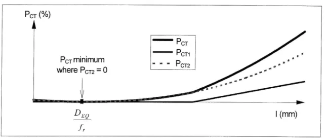
T PCTPCT minimum where PCT2 = 0
Figure 3.5 PCT on case A curves as afunction ofcant de ciency (I). Minimum PCT will be achieved at a cant de ciency according to [3.12]. The corresponding cant is arranged not to minimise PCT], the discomfort according to lateral acceleration and lateral jerk, but to avoid outward rolling of the vehicle when the effective roll factor )2 is greater than unity. For tilting trains, where the effective roll factor . is less than unity, the cant which minimises PCT is negative (l), in order to avoid inward rolling.
However, if zero cant is arranged, the PCT will deviate very little from the optimal zero value. For a transition curve which the vehicle takes 1 second to pass, the highest value of equilibrium cant DEQ according to [3.15] is 28.7 mm for a conventional vehicle with =l.2. If no cant is arranged, PCT for standing passengers will be 0.006%. According to [3.17], concerning seated passengers, the highest value of equilibrium cant is 40.3 mm for the same type of vehicle. If no cant is arranged, PCT for seated passengers will be 0.02%.
For a tilting train with effective roll factor =0.3, the highest value of equilibrium cant DEQ according to [3.14] is 34.5 mm if the vehicle takes 1 second to pass the transition curve. With zero cant, PCT for standing passengers will be 0.15%. According .to [3.16] the highest value of equilibrium cant is 48.4 mm for tilting trains. If no cant is arranged, PCT for seated passengers will be 0.02%.
These PCT values are so small and insigni cant that they cannot justify the arrangement
of cant. For longer transition curves, which the vehicle takes more than 1 second to pass,
the PCT values will be even smaller. Therefore, it may be concluded that on case A curves a suitable cant is zero.
KTH TRITA FKT Report 1997245 19 VTI Rapport 424A
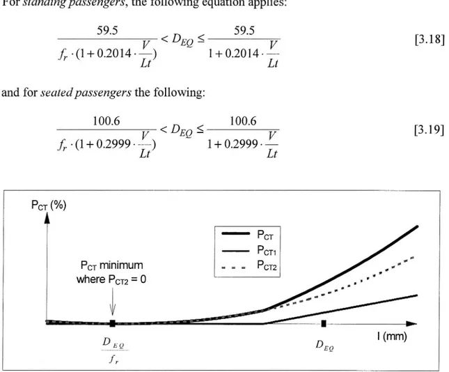
Case B curves: Low equilibrium cant
dPCTZ
In this case, the derivative is positive at the level of cant de ciency where PCT] is greater than zero according to [3.10] and [3.11] respectively, but if zero cant is arranged, PCT] is greater than zero. This case is only relevant when the effective roll factorf,. is greater than unity.
For standingpassengers, the following equation applies:
59.5
V < DEQ s
59.5V
[3.18]
- 1+0.2014- 1+0.2014 -fr ( Lt) Li and for seatedpassengers the following:
100.6
V < DEQ S
100.6V
[3-19]
. 1+ 0.2999 - ~ 1+0.2999 -fr ( Lt) LiPCT (0/0)
A
_ PCT
PCT1
PCT minimum .. .. .. Pm where PCT2 = OFigure 3.6 PCT on case B curves as a function of cant de ciency (I). When considering standing passengers, the highest level of equilibrium cant DEQ according to [3.18] is 34.5 mm if the effective roll factor equals 1.2 and if the vehicle takes 1 second to pass the transition curve. If no cant is arranged, PCT] for standing passengers will be 2.2% and PCTZ will be 0.009%. Both these values may be reduced to zero if the rolling is eliminated according to formula [3.12]. The corresponding cant D may be expressed as
l
D: 1 - -D
( f) EQ
[
3.20l
7'
20 KTH TRITA-FKT Report 1997:45 VTI Rapport 424A
In the case of an effective roll factorfr of 1.2 and a transition curve taking 1 second to pass, the highest level of equilibrium cant DEQ for seated passengers is 48.4 mm according to [3.19]. If no cant is arranged, PCT] for seated passengers will be 1.2% and PCT; will be 0.02%. These values may be reduced to zero if the rolling is eliminated according to formula [3.20].
Also these PCT values are very small. The optimal cant on case B curves deviates very little from zero cant according to [3.20], at least if the effective roll factor fr is only
slightly greater than unity. If the transition curve is longer, and the vehicle takes more
than 1 second to pass it, the highest level of equilibrium cant DEQ according to [3.18] and [3.19] will be slightly higher. If no cant is arranged, the PCTZ term will be slightly reduced, compared with the l-second transition curve, but the PCT] term is unaffected. Case C curves: High equilibrium cant
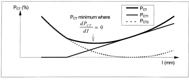
On these curves, the equilibrium cant DEQ is so high that if no rolling takes place, the PCT] term will be greater than zero, and the minimum PCT is achieved where the rst derivative ofPCT] is not continuous.
By de nition and according to [3.10] and [3.11] respectively, the optimal cant de ciency 1* for standing passengers is:
59.5
1* = V [3.21] - 1+
02014-fr (
LI)
and for seatedpassengers: 100.6 1* = V [3 .22] fr - (1 + 0.2999 - E) PCT PCT
PCT minimum where dP.. .9£ IS discontinuous. .
Figure 3. 7 PCT on case C curves as afunction of cant de ciency (I).
KTH TRITA-FKT Report 1997:45
21
Some examples of optimal cant de ciencies 1* are given, for conventional coaches (fr=1.2) in Table 3.1 and tilting coaches (72:03) in Table 3.2 on transition curves which the vehicle takes l-5 seconds to pass.
Lt=V/3 .6 Lt=V/ 1.8 Lt=V/l .2 Lt=V/0.9 Lt=V/0.72 (m-h/km) (m-h/km) (m-h/km) (m-h/km) (m-h/km)
Duration 1 sec 2 sec 3 sec 4 sec 5 sec 1* (standing) 28. 7 36.4 39.9 42.0 43.3 1* (seated) 40.3 54.4 61.6 66.0 68.9 Table 3.] Optimal cant de ciencies (mm) on case C curves for
conventional coaches with fr=1.2.
Lt=V/3.6
Lt=V/1.8
Lt=V/l.2
Lt=V/O.9
Lt=V/O.72
(mob/km)
(m-h/km)
(m-h/km)
(m-h/km)
(m-h/km)
Duration 1 sec 2 sec 3 sec 4 sec 5 sec 1* (standing) 115.0 145.6 159.7 167.9 1 73.2 1* (seated) 161.2 21 7.8 246. 6 264. 0 275.8 Table 3.2 Optimal cant de ciencies (mm) on case C curvesfor tilting
coaches withfr=0.3.
For conventional coaches (assuming an effective roll factor )3. greater than unity) the optimal cant de ciencies are quite low. Hence the limits concerning maximum cant and/or maximum cant excess (for slower trains) may require the cant de ciency to be higher than [3.21] or [3.22]. In such cases, the cant which minimises PCT is the highest permissible with regard to the limit in question. On the other hand, for tilting coaches (assuming an effective roll factor f,.=0.3) the optimal cant de ciencies for seated passengers are relatively high.
On the case C curves, the optimal cant de ciency is different for standing and seated passengers respectively. In order to maximise comfort, the cant de ciency should be in the range:
59.5
V
S I S 100.6V
[3.23]
. 1+0.2041-
.
1+0.2999-» (
Lt)
fr (
Lt)
22
KTH TRITA-FKT Report 1997:45
since a cant de ciency outside this interval results in unnecessarily high PCT values for both standing and seated passengers.
Ifthe cant is chosen to minimise PCT for standing passengers, the term PCT] will be at a minimum for both standing and seated passengers, but the PCT2 term for seated passengers will be slightly higher than its optimal value. If the cant is chosen to minimise PCT for seated passengers, the PCT; term for seated passengers will be slightly reduced, but the PCT] term for standing passengers will be higher than its optimal value. The derivatives of PCT describe the magnitude of the changes. For standing passengers
dPCT .
a I
and within interval [3.23], IS
a PCT
V = .' O.l867+0.0376-d] f] ( Lt)_
V
V
13.13-10 6. - -- D -
Lt((EQ )U)
~1-~ - 1-283
[]
3.24
dP
CT ls
.
while for seatedpassengers and within the same interval,
dP
_
V
V
w CT = 120.3.10 6 fr 'L f-((DEQ- ~1)-E)°'6z6
[325]
Some reasonable combinations of equilibrium cant DEQ and cant de ciency I show that the magnitude of [3.24] is much larger (30 100 times) than the magnitude of [3.25]. This indicates that when the cant de ciency I is altered within interval [3.23], a decrease in PCT for seated passengers must be paid for by a much larger increase in PCT for standing passengers. Hence, it seems reasonable to minimise PCT for standing passengers (according to [3.21]) rather than seated ones (according to [322]).
Case D curves: Very high equilibrium cant
In this case, the optimal cant de ciency is expected to be achieved at a higher value than [3.21] and [3.22], because a positive value of PCT] is accepted in order to achieve such a decrease in the value of PCT2 that the total PCT will be lower. The optimal cant
a PCT
de ciency is found where the derivative is zero.
KTH TRITA-FKT Report 1997:45
23
PCT (0/0) PCT PCT minimum where PC u a a. P deT = 0 CT2
wa smwmmmmn_gm mmmmusw > | (mm)
Figure 3.8 PCT on case D curves as afunction ofcant de ciency (I).
A necessary condition for this case is that the derivative
is negative at a level of I
slightly above [3.21] and [3.22], i.e. dPCT
d1
< 0
[3.26]
Equation [3.26] and a derivation of equation [3.8], concerning standing passsengers, give
all
= f,. .(o.1867+0.0376.£ )
«13.13-10 6 ~f,. .g-«DEQ f,.-I)-£)1'283 < 0
[3.27]
A simpli cation of [3.27] gives
1 Lt Lt
D
EQ f,»
.1> - 14219-- +28641-283
V (
V
)
[
3.28
]
A similar treatment of equations [3.26] and [3.9], concerning seatedpasssengers, gives
DEQ j; .1 > 51; - (488 - $5 +146)0-626
[3.29]
The highest values of the left sides of [3.28] and [3.29] will be achieved with tilting trains and typical values might be 400 mm for the rst term and 75 mm (0.3250 mm) for the second term. Some values of the right sides of [3.28] are shown in Table 3.3, for transition curves with a duration of 0.5-2.5 seconds. (Since the left sides of [3.28] and [3.29] equal the actual amount of cant if12 = 1, they are designated equivalent cant in Table 3.3.)
24 KTH TRITA-FKT Report 1997245
Lt=V/7.2
Lt=V/3.6
Lt=V/2.4
Lt=V/1.8
Lt=V/1.44
(m-h/km)
(m~h/km)
(m~h/km)
(m~h/km)
(m-h/km)
Duration 0.5 sec 1 sec 1.5 sec 2 sec 2.5 sec
Equivalent 103. 4 mm 270.] mm 494. 0 mm 771.5 mm 1099. 7 mm
cant
PCT2 20. 7% 38.1% 59. 9% 85. 9% >1 00% Table 3.3 Minimum equivalent cant (mm) on case D carves, standing
passengers.
(The corresponding values for seated passengers are higher than 700mm.)
Hence we may question whether or not it is relevant to study the case D curves. They correspond to a situation with high cant, large tilt angle and a transition curve with a shorter duration than 1.5 seconds, which leads to very high PCT values.8
Conclusions on optimal cant
Of the four different cases analysed, case A and case B are less interesting to investigate further in this study. The entire PCT function equals zero for the optimal combination of cant and cant de ciency, indicating no passenger discomfort at all. Since there is an interest in increasing the permissible train speeds (see Section 2.1), we may conclude that in cases A and B, the vehicle speed for which PCT has been calculated is too low and should be increased in the analysis (unless the speed is restricted by an adjacent curve, but then further analysis should be concentrated on that other curve). Also case D is less interesting to study, since it corresponds to a situation where high cant must be combined with very short transition curves and the corresponding PCT values are very high.
The most interesting case to analyse is case C, where the PCT function is non-zero,
indicating that the passengers perceive some level of discomfort. If possible, the cant should be so high that the PCT] term for standing passengers, representing discomfort caused by lateral acceleration and lateral jerk, equals zero.9 If the maximum value of permissible cant, or the maximum value of permissible cant excess for slower trains, limits the actual cant to a lower value, the maximum cant according to the restriction in question should be used.
8 If future research results in a new PCT function with continuous rst derivative with respect to cant de ciency, cases A, B and C will not occur and optimal cant de ciency must be calculated with the condition dPCT/dl=0.
9 It may be noticed that this decision rule corresponds fairly well with the normal cant on high speed lines in Belgium, reported by Raviart (1996), see Section 2.1.
KTH TRITA-FKT Report 1997:45 25 VTI Rapport 424A
If the actual cant is higher than the optimal cant, the corresponding PCT will be only slightly higher than its optimal value. However, according to Forstberg ( 1996), Koyanagi (1985), Ohno (1996) and Suzuki (1996), high roll velocity and/or high roll acceleration are correlated with motion sickness. Hence, the risk of motion sickness, rather than high PCT values, constitutes a reason for not using higher cant than the optimum.
Unless cant is optimised for tilting trains, the optimal tilt is not proportional to cant de ciency.10 If the control system for vehicle body tilt has delays and/or threshold values for lateral acceleration, the initial jerk on the transition curve will be higher compared to the jerk resulting from a control system which is synchronised with the transition curves. For a certain resulting lateral acceleration in the vehicle body, the roll velocities must be higher when using control systems with delays and/or threshold values compared to the roll velocities of a synchronised tilt control system. The conclusion is that the tilt control system ought to include a route le containing alignment and cant, for calculating the optimal tilt velocity in the transition curves, and that the system ought to be synchronised with the alignment.
3.3
PCT and the choice of horizontal alignment
In this section, clothoid - circle - clothoid combinations between xed straight lines are analysed. Equally costly alignment alternatives may be described by the permissible zone in the R-Lt plane, see Figures 2.5 and 2.6. The permissible zone may be de ned by the angle Aw between the straight lines and the positions (longitudinal as well as lateral) of the binding obstacles (Kufver 1997a). In order to clarify the basic relations, only one binding obstacle will be used in the analysis. The optimal solution (R-Lt combination) is expected to be located on the border which is de ned by the obstacle (see Section 2.2). The clothoids are assumed to have the same lengths, which corresponds to the most frequent situation.
The smallest radius for train speeds of 200 km/h, according to the limits in Table 2.1, and the shortest corresponding transition curve (R=1888 m and Lt=180 m) together constitute the reference alternative in the analysis. When the lengths of the transition curves are altered, the necessary adjustment of the curve radius depends on the angle All! between the straight lines and the longitudinal positions ofthe binding obstacles (Kufver 1997a). For a certain change in transition length, a smaller angle Aw requires a larger adjustment of radius than a larger angle Aw. Concerning the positions of the obstacles, there are two extremes. An obstacle in the middle of the curve requires the smallest adjustment of curve radius, while an obstacle on an adjacent straight line (i.e. a turnout which should not be placed on a curve) requires the largest adjustment.
Each alignment alternative (R Lt combination) will be evaluated with its optimal cant. All alternatives are case C curves (see Section 3.2). At low train speeds, some of the
10 For case C curves, re-arrange equation [3.21] and express an optimal effective roll factorf,.* as a function ofI, V and Lt.
26
KTH TRITA-FKT Report 1997:45
alternatives have the optimal cant de ciency according to [3.21], but at higher train speeds, the cant is limited to 150 mm.11
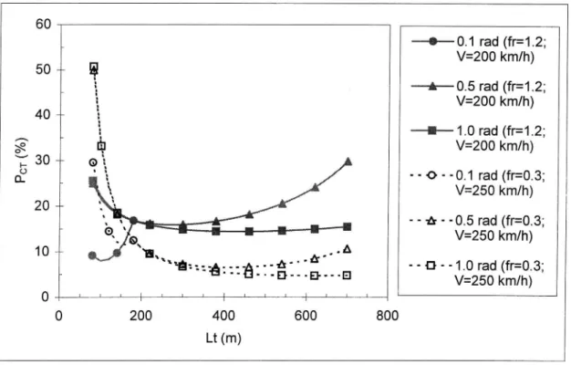
Figures 3.9-3.12 show PCT for standing passengers on horizontal curves with a change
in direction Aw of 0.1 rad and 0.5 rad, and with a binding obstacle at the midpoint and at
the endpoint of the curve respectively. The longest transition curve which may be used depends on the change in direction and the binding obstacles, since the length of the circular curve must be greater than (or equal to) zero, see Figure 2.6. The gures show PCT as functions of the lengths of the transition curves for different train speeds and for different effective roll factors (0.3 for tilting trains and 1.2 for conventional trains).12
4O WmfF l .2; 35 V=160 km/h 30 w «we-mfr=1.2; * V=200 km/h 25 -g\: 20 _: mefz; '5 V=220 km/h CL _ 15 _ - - I - -fr=O.3;
10 ___
V=220 km/h
5__ . ~.____ --*--fr=0.3;""-I----I
V=250km/h
O 1 x l ' . 1"} g} i} 1 50 100 150 200Lt (m)
Figure 3.9 Simplified PCTfor standing passengers on a curve with A ra=0.1 rad and a midpoint obstacle.
11 Some railway companies accept higher cant than 150 mm. According to Goldenbaum and Meyer (1985), Italy and Poland accept 180 mm of cant, while France and Japan accept 200 mm.12 . . . . . . .
Correspondmg curve radu and cant de c1enc1es are shown 1n Appendlx 5.
KTH TRITA-F KT Report 1997 :45 27 VTI Rapport 424A
4O - Wmfr .2; 35 V=160 km/h 30 ~ WfFLZ; ~ V=200 km/h 25 ~~
c}: 20 #
wmwfr=1.2;
5 V=220 km/h CL _ 15 ~ _ - - I - -fr=0.3;1O __
v=220 km/h
5 __ - - -A- - -fr=0.3; V=250 km/h 0 50 200Figure 3.10 Simplified PCTfor standing passengers on a curve with A w=0.1 rad and an endpoint obstacle.
80 wwfr=1.2; 7O V=160 km/h
60 "
Mew-fr z;
' V=200 km/h 50 -c}: 40 _: wwfr=1.2;5
v=220 km/h
LL _30
- - I - -fr=0.3;
20 W1o--
_
"
l.
1..
"" --*--A--'A"*""
_..-A
--*--fr=0.3;
V=250 km/h
0 200 400 600 800 Lt (m)
Figure 3.11 Simplified PCTfor standing passengers on a curve with A ga=0.5 rad and a midpoint obstacle.
28 KTH TRITA-FKT Report 1997245
wwfr .2; V=160 km/h wwwfr=1.2; V=200 km/h
e",
5
me .2;
V=220 km/h
0. - I - -fr=O.3; V=220 km/h - - at - -fr=O.3; V=25O km/h 800Figure 3.12 Simplifed PCTfor standing passengers on a curve with A w=0.5 rad and an endpoint obstacle.
Figures 3.13-3.14 show PCT as functions of the lengths of the transition curves for different changes in direction between the straight lines Aw. The speed of the tilting coaches ( =0.3) is 250 km/h and the speed of the conventional coaches ( r "1.2) is
200 km/h.13
13 Corresponding curve radii and cant de ciencies are shown in Appendix, 5.
KTH TRITA-FKT Report 1997245 29
6O
40
- 0.1 rad (fr=1.2; V=200 km/h) 0.5 rad (fr=1.2; V=200 km/h) - 1.0 rad (fr=1.2; V=200 km/h)§
7: 30
Cf - O - -O.1 rad (fr=0.3;v=250 km/h)
20 -~- a - -o.5 rad (fr=0.3;
v=250 km/h)
10 w
E:-_- ;-_-
"
A "
--E}--1. ra (r=0.3;
o d f
19'
a
D "E" '3'
v=25o km/h)
0 : : ' : O 200 400 600 800 Lt (m)Figure 3.13 Simpli ed PCTfor standingpassengers on curves with A 1//=0.I-1.0 rad and a midpoint obstacle.
60 0.1 rad (fr=1.2;
V=200 km/h)
50 -ww w05 rad (fr=1.2; V=200 km/h)40
'- ~ 1.0 rad (fr=1.2;g
V=200 km/h)
1: 3o
-cf - o - -O.1 rad (fr=0.3;v=25o km/h)
20 ~
- -A - -O.5 rad (fr=0.3;v=250 km/h)
10 ~-- El ~-- ~--1.0 rad (fr=0.3;v=250 km/h)
0 % I ' ' l O 200 400 600 800 Lt (m)Figure 3.14 Simplified PCTfor standing passengers on curves with A w=0.1-1.0 rad and an endpoint obstacle.
30 KTH TRITA-FKT Report 1997245
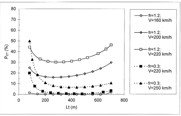
Concerning Figures 3.9-3.14, the following remarks and conclusions may be made: The optimal lengths of the transition curves depend on the positions of the binding
obstacles. A midpoint obstacle favours longer transition curves than an endpoint
obstacle does. Kufver (1997b) draw the conclusion that when changing the transition lengths, midpoint and endpoint obstacles constitute the extreme cases where the smallest and largest compensations of horizontal radius are needed, respectively. Hence,
the midpoint and endpoint obstacles also de ne the extreme cases when calculatingPCT.
The optimal lengths of the transition curves depend on the effective roll factor)2, which considers the roll coef cient of the vehicle and a possible body tilt system. The price which has to be paid when lengthening the transition curves, i.e. the reduction in the horizontal radius, affects PCT less if the effective roll factor is low. Hence, at a certain
train speed, lower effective roll factors favour longer transition curves than higher
effective roll factors. (For the same reason, if the limit for cant is raised above the present Swedish limit of 150 mm, the optimal transition length will be increased.) The magnitude of the change in direction between the straight lines Aw also affects the optimal lengths of the transition curves. Regardless the position of the binding obstacle, a larger angle Aw requires smaller changes in the horizontal radius for certain changes in transition length, compared to those at a smaller angle. Hence, for large angles All! the optimal transition curves will be longer.
The optimal transition lengths for conventional coaches are in some cases relatively short (see Figure 3.14). All PCT values with shorter transition curves than 180 m refer to a rate of cant higher than the present limit of 46 mm/s.l4 Hence, if this constraint is not relaxed, the resulting PCT values will be higher and the optimal transition curves longer.
The train speed affects the optimal length of the transition curves in a complex manner. If the train speed is relatively low, e.g. 160 km/h for a conventional coach in Figures 3.11 and 3.12, some alignment alternatives have cant according to [3.21], which means the passenger discomfort is caused by the rolling alone. In these cases, PCT slowly decreases with increased transition length as long as the PCT] term (discomfort caused by lateral acceleration and lateral jerk) is zero. When PCT] becomes positive (see Lt=340m for the conventional coach at 160 km/h in Figure 3.12), the entire PCT function starts to increase quite rapidly.
At higher train speeds, the optimal transition length is shorter and its dependence on train speed is not very strong. The optima are usually quite at, hence slightly non-optimal transition lengths do not affect PCT very greatly.
Nevertheless, the optimal transition lengths for tilting coaches deviate relatively greatly from the 180 m reference alternative (except at small angles, such as Aw=0.1 rad). In
14 The potential bene t of an increased rate of cant has already been reported by Harborough (1986) and UIC (1991).
KTH TRITA FKT Report 1997:45 31 VTI Rapport 424A
Figure 3.13, PCT in a tilting coach is about 12.5% at the reference alternative (Lt=180 m) but may be reduced to PCT values of 55-65% at Lt=400 m for curves with angles in the interval 0.5 radgAxngO rad. Since high roll velocities (and/or high roll accelerations) are correlated to motion sickness, there is an interest in reducing the roll velocities by a reduced body tilt and/or optimised transition curves. Both methods usually increase the lateral acceleration (when obstacles are considered), but modifying the alignment results in a lower lateral acceleration than reducing the tilt.
Another important conclusion is that, since the optima are at for the lower train speeds,
there is no great disadvantage for trains at such speeds if the transition lengths are optimised for higher speeds.
When the track is used for conventional as well as tilting trains, the optimal transition lengths may differ considerably. However, optima are at and reasonable compromises may be found.
The alternatives with shorter transition lengths than in the reference alternative result in larger radii and larger cant excess for freight trains (trains with a lower speed than the equilibrium speed).
32 KTH TRITA-FKT Report 1997:45 VTI Rapport 424A
4.
Models for dynamic track/vehicle analysis
4.1
GENSYS multibody computer code
In the dynamic track/vehicle analysis, simulations have been conducted with the multibody computer code GENSYS. The code is general and may be used in a wide range of dynamic applications (Lange 1996, Persson 1995b). In the eld of railway dynamics, there are several options concerning the number of degrees of freedom for the individual bodies, types of vehicle coupling elements, types of wheel/rail contact kinematics, type of analysis phase (time domain simulations, frequency domain simulations, quasi-statical analysis), etc.
In this study, simulations are conducted in the time domain. Vehicles bodies, bogies and wheelsets are modelled as rigid bodies and have six degrees of freedom each (three translations and three rotations). The track is modelled as lumped masses, connected by the contact areas to the wheelsets. Each track mass has only one degree of freedom: lateral translation. Hence, there are 46 degrees of freedom for each vehicle.
Lateral [ 9 G
/// ///////// /////
Figure 4.] Degrees offreedom in this study.
KTH TRITA-FKT Report 1997245 33 VTI Rapport 424A