S
CHOOL OF
I
NNOVATION
,
D
ESIGN AND
E
NGINEERING
V
ÄSTERÅS
,
S
WEDEN
Thesis for the Degree of Bachelor in Computer Science – 15.0 hp
NSGA
-
II DESIGN FOR FEATURE SELECTION
IN EEG CLASSIFICATION RELATED TO
MOTOR IMAGERY
Robin Johansson
rjn16002@student.mdh.se
Examiner:
Ning Xiong
Mälardalen University, Västerås, Sweden
Supervisor: Miguel León Ortiz
Mälardalen University, Västerås, Sweden
Abstract
Feature selection is an important step regarding Electroencephalogram (EEG) classification, for a Brain-Computer Interface (BCI) systems, related to Motor Imagery (MI), due to large amount of features, and few samples. This makes the classification process computationally expensive, and limits the BCI systems real-time applicability. One solution to this problem, is to introduce a feature selection step, to reduce the number of features before classification. The problem that needs to be solved, is that by reducing the number of features, the classification accuracy suffers. Many studies propose Genetic Algorithms (GA), as solutions for feature selection problems, with Non-Dominated Sorting Genetic Algorithm II (NSGA-II) being one of the most widely used GAs in this regard. There are many different configurations applicable to GAs, specifically different combinations of individual representations, breeding operators, and objective functions. This study evaluates different combinations of representations, selection, and crossover operators, to see how different combinations perform regarding accuracy, and feature reduction, for EEG classification relating to MI. In total, 24 NSGA-II combinations were evaluated, combined with three different objective functions, on six subjects. Results shows that the breeding operators have little impact on both the average accuracy, and feature reduction. However, the individual representation, and objective function does, with a hierarchical, and an integer-based representation, achieved the most promising results regarding representations, while Pearson’s Correlation Feature Selection, combined with k-Nearest Neighbors, or Feature Reduction, obtained the most significant results regarding objective functions. These combinations were evaluated with five classifiers, where Linear Discriminant Analysis, Support Vector Machine (linear kernel), and Artificial Neural Network produced the highest, and most consistent accuracies. These results can help future studies develop their GAs, and selecting classifiers, regarding feature selection, in EEG-based MI classification, for BCI systems.
Table of Contents
1.
Introduction ... 5
2.
Background ... 7
2.1.
Supervised Learning ... 7
2.1.1.
K-Nearest Neighbor ... 7
2.1.2.
Support Vector Machine ... 8
2.1.3.
Linear Discriminant Analysis ... 11
2.1.4.
Artificial Neural Network ... 12
2.2.
Feature Reduction ...15
2.3.
EA ...15
2.4.
GA...16
2.4.1.
Initialization... 16
2.4.2.
Selection ... 16
2.4.3.
Crossover ... 17
2.4.4.
Mutation ... 19
2.4.5.
Replacement ... 19
2.4.6.
Termination ... 20
2.5.
Multi-Objective Optimization ...20
2.5.1.
NSGA ... 21
2.5.2.
NSGA-II... 22
3.
Related Work ... 25
3.1.
Related Studies ...25
3.2.
Individual Representation...26
3.3.
Breeding Operators ...26
3.4.
Objectives ...27
3.5.
Classifiers ...28
4.
Problem Formulation ... 29
4.1.
Limitations ...29
5.
Method ... 30
6.
Ethical and Societal Considerations ... 31
7.
Design and Implementation ... 32
7.1.
Representations ...32
7.1.1.
Hierarchical Representation (HR) ... 32
7.1.2.
Non-hierarchical Representation (NHR) ... 33
7.1.3.
Gonzalez Representation (G30 & G600) ... 33
7.2.
Breeding Operators ...33
7.2.1.
Selection ... 33
7.2.2.
Crossover ... 35
7.2.3.
Mutation ... 37
7.3.
Objective Functions ...38
7.4.
Classifiers ...38
8.
Experiment Settings ... 40
8.1.
NSGA-II Settings ...40
8.1.1.
Hierarchical settings: ... 40
8.1.2.
Non-Hierarchical settings: ... 40
8.1.3.
González settings: ... 40
8.2.
Classifier Settings ...40
8.2.1.
Support Vector Machine settings: ... 40
8.2.2.
Linear Discriminant Analysis settings: ... 41
8.2.3.
Artificial Neural Network:... 41
8.2.4.
K-Nearest Neighbour Settings: ... 41
9.
Results ... 42
9.1.
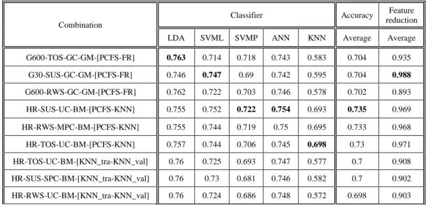
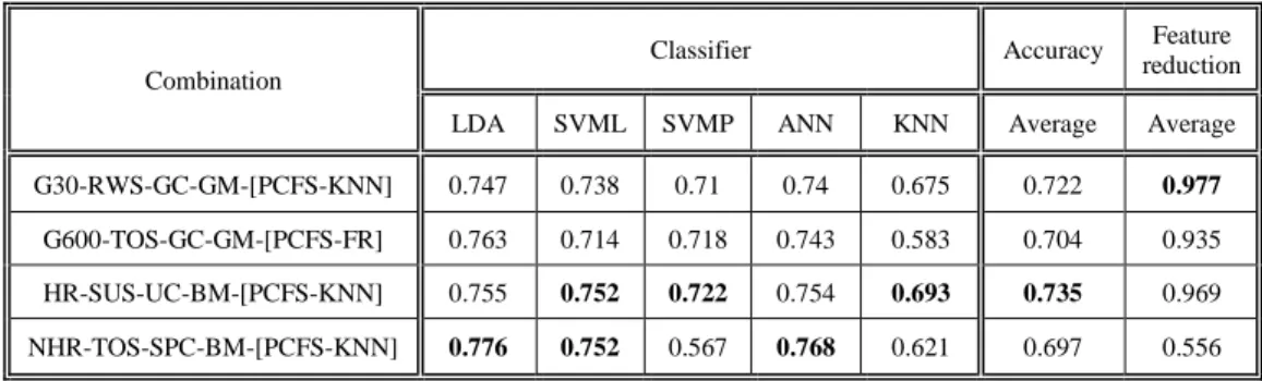
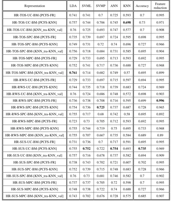
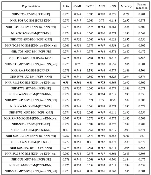
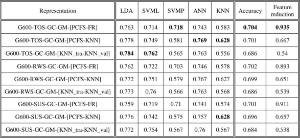
Comparison between representations & objectives ...42
9.2.
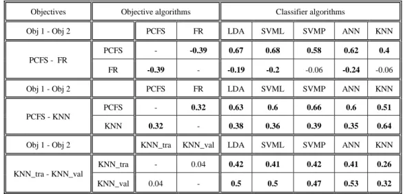
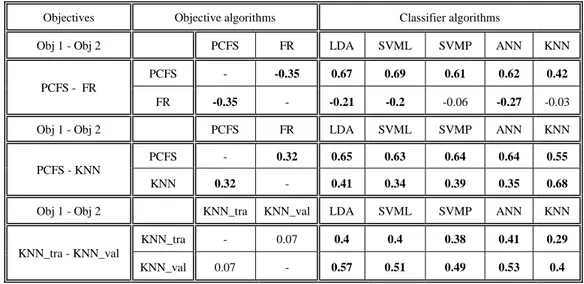
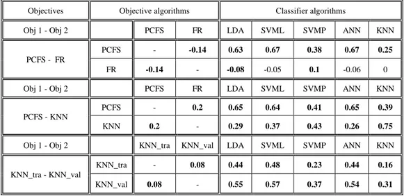
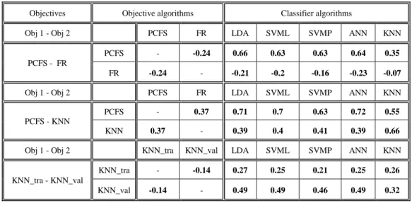
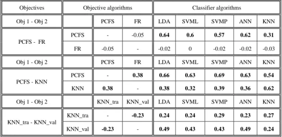
Correlation between objectives & classifiers ...44
9.3.
Statistical validation...45
9.4.
Comparison to reference studies ...46
10.
Discussion ... 47
10.1. Representations ...47
10.2. Breeding Operators ...47
10.3. Objectives ...47
10.4. Classifiers ...48
10.5. Contributions ...48
11.
Conclusions ... 49
12.
Future Work ... 50
13.
References ... 51
Appendix A ... 53
A.1 Comparison between representations & objectives ...53
A.2 Correlation between objectives & classifiers ...56
1. Introduction
Brain Computer Interface (BCI) is a communication interface between a brain and an external device [1]. Since
brain activity produces electrical signals that are measurable from the outside of a person’s head, we can feed the signals to a BCI, that translates the electrical signals and converts them to commands for the external device. A person can then interact said electrical device with their mind. It is commonly used in medicine as aid, or treatment for different disabilities and disorders. An example being NeuroFeedback (NF) [2], where a BCI system is used in combination with Motor Imagery (MI) to measure, and display brain activity in real-time on a screen, or as audio feedback. MI, being defined as a mental simulation of a motor action, has proven to share similar neural activity to an actual motor action [3], and when recorded, can be recognized by the BCI, and visualized on a screen in real-time for a patient to view [2]. This can be used to train your brain and gain control over involuntary activities. In paper [2], they highlight some experiments done to try NF as treatment for Attention Deficit Hyperactivity Disorder (ADHD), and to help with rehabilitation after stroke. For people with ADHD it has been observed that they have higher amplitudes of low frequency (theta and delta waves) in their resting state, which are associated with relaxation. NF can be used to try and gain control, and lower these frequencies by looking at a screen with real-time feedback, and try to alter them. Thus, NF relies heavily on giving feedback in real-time, which is proven in [4], where they explain that delay between the neural activity, and the feedback from NF decreases the learning and rehabilitation capabilities.
The most common technology to measure, and record brain signals is Electroencephalography (EEG) [5]. This is because the equipment is not to expensive compared to other methods. Multiple electrodes are placed directly on the scalp of a person, unlike other methods where they have to be inserted by surgery. EEG is therefore seen as the most non-invasive method. The electrodes record the electrical activity over a period of time, which can then be stored in computer memory [5]. A drawback off EEG is that a sample recorded with this method often consist of a large number of features from multiple recording channels, and due to fatigue of the user, only a limited number of samples can be recorded [6], [5], [7]. This combination is not good when used as input for classification due to over-fitting problems (i.e when a model has “memorized” the noise and will perform well on its training data, but very poorly on novel data). EEG also record a lot of noise due to a problem called volume conduction [8]. In [7], and [9], they use Support Vector Machine (SVM) as classifier, because it works well with lots of features and few samples. Unfortunately, it takes a long time to compute, and as explained earlier, applications like NF need to have the data in real-time. Therefore, a feature selection step is required, which is a method of reducing the number of features, and only use a small subset that provide relevant and non-redundant information to the classification, and as a result, reduces the computational time [6], [7]. Feature selection is not an easy task since you need to find the features that are important to the classification, and distinguish them from the noise, otherwise the prediction accuracy will decrease [6], [7].
To find the important features, other studies have found that Evolutionary Algorithms (EA) are a good choice, and the most common algorithm used, is Genetic Algorithm (GA) [6]. This is a metaheuristic optimization algorithm based on biological evolution, with breeding operators such as selection, crossover, and mutation. It modifies a population of individual solutions over generations, with the goal of evolving the solutions over time, towards an optimal solution. The problem with a regular GA, or any other regular EA, is that it only works well for one objective, and feature reduction in this case have multiple objectives, reduce features, and not lower the accuracy. These two objectives are conflicting in the sense that if we reduce the features too much, the accuracy decreases, and if we focus only on the solutions with high accuracy, then the number of required features will rise. Therefore, a special version of EA must be used, a multi-objective evolutionary algorithm (MOEA), which can optimize multiple conflicting objectives simultaneously.
In [10], the research team did a comparison between a MOEA, and two single-objective algorithms, for a feature reduction problem related to EEG classification. The MOEA used was Non-Dominated Sorting Genetic Algorithm
II (NSGA-II), and the single-objective GAs were, Steady Sate GA (SGA), and a regular GA. They showed that
NSGA-II both had higher accuracy, and feature reduction, in comparison to the other two, with a slight drawback of being much slower to converge compared to SGA. In [6], another team created a novel version of NSGA-II, to solve a similar feature selection problem. The algorithm was compared to two other proven methods, and did produce a very promising result. Christoffer Parkkila continued the work from [7] in his bachelor thesis [9], where they had used a novel single-objective GA called Hierarchical Genetic Algorithm (HGA) for feature selection. He implemented a MOEA to be used instead of the HGA used previously. The MOEA he implemented was NSGA-II [9], and it was able to improve the result of the previous study. Many studies have used NSGA-NSGA-II for similar
problems [6], [9], [10], [11], showing that the algorithm is a good choice for a feature selection problem related to EEG classification. However, there is still room for improvement, as explained earlier, to make NF efficient we need to keep the computational time as low as possible, since NF relies on giving feedback in real-time [2], [4], [7]. A low computational time requires a fast classification system, which requires good feature selection. Since NSGA-II have proven to be a great solution to this problem, the purpose of this study is to improve the algorithm even further. NSGA-II has not yet been evaluated with different combinations of individual
representations and different breeding operators, which this study aims to evaluate, in hopes of improving the
prediction accuracy, for a smaller number of used features, which in turn will decrease the computational time. Three different individual representations, three selection, and three crossover operators will be tested for the original NSGA-II, and compared to the modified NSGA-II from [6], which will also be tested with the implemented selection operators. All combinations will be tested with three different objective-function pairs,
Pearson with Feature Reduction (Pearson-FR) from [7], Pearson with k-nearest neighbor (Pearson-kNN) from
[9], and Training-validation percentage with kNN, from [6]. To evaluate the results, five different classifiers will be used.
The paper is organized as follows: In Section 2, all necessary theory is presented, that is needed to understand this study. In Section 3, some of the related works in this field are presented, and discussed. Section 4 describes the problem more thoroughly, and the research questions are defined. In Section 5, the methods of research are provided, and in Section 6, the ethical considerations are presented. In Section 7, the system design, and implementation, are described, with the experiment settings being provided in Section 8. In Section 9, the experiment results are provided, and in Section 10, the results are discussed. Finally, Section 11 concludes the work, and future work is provided in Section 11.
2. Background
In this section, all the necessary theory, regarding the study are presented, and it is organized as follows: In Section 2.1, supervised learning, and related algorithms are described. In Section 2.2, the concept of feature reduction is explained, and in Section 2.3, the concept of evolutionary algorithms are described. In Section 2.4, a specific type of evolutionary algorithms is explained, namely, Genetic Algorithm. Finally, in Section 2.5, Multi-Objective problems are described, with NSGA, and NSGA-II being highlighted as solutions.
2.1. Supervised Learning
Supervised Learning is a subcategory of Machine Learning, commonly used for prediction problems [12]. The
algorithms are building a mathematical model, by learning from known, labeled data. A supervised learning algorithm can either be classified as Parametric, or Non-Parametric [13]. Parametric algorithms try to simplify the structure of the problem according to a set of finite parameters, no matter how much data you input, the parameters will always be of the same amount. Usually, these parameters involve the mean, and standard deviation of normal distribution. A non-parametric algorithm does not have a fixed number of parameters. The complexity of the mathematical model depends on the amount of input data, by increasing the amount of input data, the amount of parameters required also increases. For parametric models, you only need to know the parameters of the mathematical model to classify new data, while non-parametric methods instead use the training data directly in the classification, by finding similar patterns between the input data, and the labeled training data. This means that a non-parametric algorithm always needs to keep the training data, while a parametric algorithm doesn’t [13]. A supervised learning algorithm learn by classifying training data, which consists of sets of input features, and the correct outputs (labels) for each set [12]. By classifying the training data, they then have the ability to look at the correct label, and use that information to tune the underlying mathematical model. The goal of the training process is to improve the mathematical model so they later can classify novel data (i.e data they have not seen before, without correct labels). A set of features can also be called a data point, instance, or sample, which can be defined as 𝑋 = {𝑓1, 𝑓2, … , 𝑓𝑛}, where 𝑓𝑖 is a feature belonging to sample X, and n is the total number of features [12]. To calculate an algorithms prediction accuracy for novel data, cross-validation is commonly used [12]. The input data sets are divided into groups, where one group is used for training, and the other is used for validation [12]. Usually, this is done in multiple rounds, called a fold, where the dataset is divided in groups differently each time. Some common supervised learning algorithms are k-Nearest Neighbor (KNN), Support Vector Machines (SVM), Linear Discriminant Analysis (LDA), and Artificial Neural Network (ANN) [12].
2.1.1. K-Nearest Neighbor
K-nearest neighbor (KNN) is a non-parametric, supervised learning algorithm [12]. A non-parametric algorithm
uses the training sets directly to classify novel data. The algorithm considers a sample to be point in a n dimensional space, where the number of dimensions (n) corresponds to the number of features that constructs the sample. This algorithm is based on the assumption that similar data points exist close to each other. When assigning a class to an input sample x, it finds the 𝑘 ∈ ℕ closest points to x in the training data sets, and assign x the class that is most common between the k closest points.
There are multiple ways to calculate the distance between two samples, with the most common method being the
Euclidean Distance (ED) [12]. It is defined as follows:
𝐸𝐷(𝑋, 𝑌) = √∑(𝑥𝑖− 𝑦𝑖)2 𝑛
𝑖=1
Where X, and Y, are two samples, n is the number of features in each set, 𝑥𝑖 is a feature from X, and 𝑦𝑖 is a feature from Y. Figure 1 shows an activity diagram over the algorithm:
The algorithm starts by initializing k, the number of neighbors to use [12]. Then it goes through all training samples 𝑌𝑖, and calculates the distances between them, and the input sample X. When all distances have been calculated, they get sorted in an ascending order. Then the algorithm takes the first k samples, and look at what their labels are. The most common label will get assigned to X. Figure 2 illustrates how it can look with k = 5, and two features. The red circle looks at the 5 closest instances, and since four of them are blue, it will be assigned class 1.
2.1.2. Support Vector Machine
Support Vector Machine (SVM) is a non-parametric, supervised learning algorithm [12]. This algorithm is able to
classify between two different classes, making it a binary classifier. It works by dividing the training samples with a hyperplane, which is placed in the middle of two classes, with as much margin between the classes, and the hyperplane as possible [13]. This is calculated by using support vectors, which are vectors that defines the maximum space between the two classes. The support vectors are essentially the samples from each class, that are closest to the opposing class. With these vectors, the hyperplane can be calculated, and placed in the middle of the
Figure 2: Example of KNN with k=5, and 2 features. Figure 1. KNN activity diagram.
resulting area, which will give the maximum margin to both classes. The algorithm can then use this plane to assign new samples a class, depending on which side of the hyperplane the point lands on. The dimension (n) of the hyperplane depends on the number of features (k) in a sample, where 𝑛 = 𝑘. In a 2-dimensional space the hyperplane becomes a line, this is illustrated by Figure 3.
To then classify a new sample, the algorithm can use the following equation [13]:
𝑓(𝑋) = 𝜔0+ 𝜔1𝑥1+ ⋯ 𝜔𝑛𝑥𝑛 ( 2 )
Which simply is a linear equation, that works for any number of features and dimensions (n) [13]. In EQ. ( 2 ), 𝜔𝑖 are the coefficients of the hyperplane, and 𝑥𝑖 represents a feature of sample X. Since it’s a binary classifier, only two labels are needed, the label (𝑦) for a sample, 𝑋𝑖, is therefore defined as: 𝑦𝑖∈ {−1,1}. To know what class X belongs to, the algorithm only has to look at the sign of EQ. ( 2 ), if 𝑓(𝑋) > 0, it belongs to class 2 (𝑦𝑖= 1), and if 𝑓(𝑋) < 0 it belongs to class 1 (𝑦𝑖= −1). To determine the distance of sample X from the hyperplane, it can calculate |𝑓(𝑋)|, which can be used as a confidence measure, where the algorithm is more confident the further away from the hyperplane X resides. However, this approach only works if the boundaries between the two classes are linear.
As previously mentioned, the hyperplane should be placed in a way that it is in the perfect middle of the two classes, with as much margin between them as possible [13]. To find this plane, we have to solve an optimization problem, where we want to maximize the margin width (M). M then relates to the hyperplane vector 𝜔⃗⃗ , where it is placed, and in what direction it points towards, which means that to maximize M, the algorithm needs to find the optimal hyperplane coefficients 𝜔𝑖. At the same time, we want to keep the constraints of 𝑓(𝑋) > 0, and 𝑓(𝑋) < 0, which are used to differentiate between the two classes. This gives the optimization problem:
Figure 3. Simple illustration of a 2-dimensional hyperplane, highlighting the margin, support vectors, and the hyperplane. The samples on the smaller lines, are the support vectors.
𝑚𝑎𝑥𝑖𝑚𝑖𝑧𝑒 𝑀 𝜔0, 𝜔𝑖, … , 𝜔𝑛, 𝜇1, 𝜇2, … , 𝜇𝑝 ( 3 ) 𝑠𝑢𝑏𝑗𝑒𝑐𝑡 𝑡𝑜 ∑ 𝜔𝑗2 𝑛 𝑗=1 = 1, ( 4 ) 𝑦𝑖(𝜔0+ ∑ 𝜔𝑗𝑥𝑗 𝑛 𝑗=1 ) ≥ 𝑀(1 − 𝜇𝑖), ( 5 ) 𝜇1≥ 0, ∑ 𝜇𝑖≤ 𝐶 𝑝 𝑖=1 ( 6 )
In this optimization problem, EQ. (3) tells us what we are optimizing, which is the margin (M) [13]. M is optimized by tuning the parameters 𝜔𝑖, and 𝜇𝑖, where 𝑤𝑖 are the hyperplane coefficients, and 𝜇𝑖 are slack variables, which corresponds to the distance of sample 𝑋𝑖 relative to the margin (M). EQ. ( 4 ) together with EQ. ( 5 ) ensures that most of the training samples will be on the correct side of the hyperplane, with a minimum distance of M. In EQ. ( 5 ) we can see the linear equation from EQ. ( 2 ) inside the parentheses. Variable 𝑦𝑖 will be the resulting class label, 𝑦𝑖∈ {−1, 1}, and from 𝑀(1 − 𝜇𝑖), we can see that some solutions will be allowed on the wrong side of the margin (if the corresponding slack variable 𝜇𝑖> 0). To find the optimal plane, all samples have to pass the criteria of EQ. ( 5 ), which means that a sample with label 𝑦𝑖= −1 need to have a negative distance from the plane, where 𝜔0+ ∑𝑛𝑗=1𝜔𝑗𝑥𝑗 produces a negative number . This means that if a solution is on the wrong side of the hyperplane, the equation criteria will not be met, and the position of the plane have to be changed [13]. The slack term in EQ. ( 5 ) ensures that some terms will be allowed inside of the margin area, since 𝜇𝑖 will be > 1, and 𝑀(1 − 𝜇𝑖) will be smaller than the margin itself (M), and because of this, samples closer to the plane will be allowed since the right side of EQ. ( 5 ) will be smaller. EQ. ( 6 ) is the penalty of misclassification, 𝜇1≥ 0 ensures that the slack variable will be positive, and ∑ 𝜇𝑖≤ 𝐶
𝑝
𝑖=1 is the amount of penalty, which is the sum of all slack variables. It also limits the amount of slack to C, which is a tuning parameter, commonly chosen by cross-validation. If a sample is on the correct side of the margin, the slack term 𝜇𝑖= 0. If 𝜇𝑖> 0 the sample is on the wrong side of the margin, and if 𝜇𝑖> 1, then it is on the wrong side of the hyperplane, which will penalize even more [13]. With C you can therefore decide how much classification error the algorithm should allow, and a bigger C will result in a bigger margin, with higher bias. A small value for C will result in a narrow margin, with lower bias probability, but higher variance. EQ. ( 3 )-( 6 ) can be written in a more compact equation, similar to a linear regression problem:
𝑚𝑖𝑛𝑖𝑚𝑖𝑧𝑒 𝜔0, 𝜔𝑖, … , 𝜔𝑛{∑ 𝑚𝑎𝑥[0, 1 − 𝑦𝑖𝑓(𝑋𝑖)] + 𝐶 ∑ 𝜔𝑗 2 𝑛 𝑗=1 𝑝 𝑖=1 } ( 7 ) 𝑓(𝑋𝑖) = 𝜔0+ ∑ 𝜔𝑘𝑥𝑘 𝑛 𝑘=1 ( 8 )
Where 𝑚𝑎𝑥[0,1 − 𝑦𝑖𝑓(𝑋𝑖)] is called a hinge loss function, which is 0 if the sample is on the correct side of the margin, otherwise the value is related to the distance from the margin [13]. The second term 𝐶 ∑𝑛𝑗=1𝜔𝑗2 corresponds to the penalty, where a large C results in smaller 𝜔𝑘, with more misclassifications allowed. EQ. ( 8 ) is the linear equation from EQ. ( 2 ), which is used both for the optimization of the hyperplane, and when we want to classify new samples. The above optimization is called a Quadratic Programming (QP) problem. This is a complex area in itself, and won’t be described in this paper. One can solve such optimization problem with for example Platt’s Sequential Minimal Optimization algorithm (SMO). For a detailed explanation of this algorithm, and how to solve these problems, I refer you to [14].
For a non-linear boundary, where samples are mixed in a way where no straight line can divide the two classes, the method gets more complicated [13]. In a case such as this, the algorithm uses kernels. A kernel is a method of transforming the feature space to a higher dimension, where the two classes now can be divided by a hyperplane of a higher dimension. The hyperplane itself is of dimension n-1, which in a 2D feature space is a line (1D), and in a 3D feature space it is a 2D plane. When transforming back to the original feature space, the hyperplane will
look non-linear, and may be curved in different ways. To solve this, we need to change the linear equation, and give it the ability to enlarge the feature space, using higher-order functions. This is done by using kernels. By looking at the behavior of EQ. ( 7 )( 8 ) , it has been found that only the inner products between the samples are needed, and only from the samples that act as support vectors. Therefore, the linear classifier from EQ. ( 8 ) can be rewritten as:
𝑓(𝑋𝑖) = 𝜔0+ ∑ 𝛼𝑘〈𝑋, 𝑌𝑘〉 𝑛
𝑘=1
( 9 )
Where 𝛼𝑘 are parameters that will be found, and optimized when inserting EQ. ( 9 ) into the optimization equation EQ. ( 7 ). These parameters will be 0 for all solutions on the right side of the hyperplane, which indicates that only the support vectors affect the optimization, both for the hyperplane, and when classifying new samples. Lastly, 〈𝑋, 𝑌𝑘〉 is the inner product between samples, X, and Y, defined as:
Linear Kernel 〈𝑋, 𝑌𝑘〉 = ∑ 𝑥𝑖𝑦𝑖 𝑝 𝑖=1
( 10 )
Putting EQ. ( 9 ) and ( 10 ) together gives us the same linear classifier as EQ. ( 8 ). A kernel is actually the inner product part, and EQ. ( 10 ) is the linear kernel. A kernel K(X, Y), is in fact:
𝐾(𝑋, 𝑌) = 〈𝑋, 𝑌〉 ( 11 )
The equation used for inner product calculation is therefore known as the kernel. Two other popular kernels are the Polynomial Kernel (PK), and the Radial Basis Function Kernel (RBF):
Polynomial Kernel 𝐾(𝑋, 𝑌𝑖) = (1 + ∑ 𝑥𝑗 𝑛 𝑗=1 𝑦𝑗) 𝑑 ( 12 )
Radial Basis Function Kernel 𝐾(𝑋, 𝑌𝑖) = 𝑒𝑥𝑝 (−𝛾 ∑(𝑥𝑗𝑦𝑗) 2 𝑛
𝑗=1
) ( 13 )
The polynomial kernel is almost identical to a linear kernel, in fact, if parameter d is equal to 1, it is a linear kernel. Otherwise, using 𝑑 > 1 transforms the feature space to a higher dimension, and involves polynomials of degree
d. The optimal value for this parameter is usually found by cross-validation.
Radial basis function kernel calculates the relationship between two samples in a higher dimension, without actually transforming it. This process is also referred to as Kernel Trick, which avoids the math of actually transforming, and saving some computations needed. In this kernel, 𝛾 is the parameter, which is a positive constant. An interesting behaviour of this kernel, is that it works somewhat similar to KNN, where only the closest samples have an effect on the classification process, when classifying a new sample X.
In summary, EQ. ( 7 ) is used to find the optimal hyperplane, and support vectors, where the function 𝑓(𝑋) defines the hyperplane, and is used when classifying new samples. That function is defined as:
𝑓(𝑋𝑖) = 𝜔0+ ∑ 𝛼𝑘𝐾(𝑋, 𝑌𝑘) 𝑛
𝑘=1
( 14 )
Where 𝐾(𝑋, 𝑌𝑘) can be either of EQ. ( 10 ), ( 12 ), or ( 13 ).
2.1.3. Linear Discriminant Analysis
Linear Discriminant Analysis (LDA) is a parametric, supervised learning algorithm [12]. This method tries to find the linear combination of features that best separates multiple classes. LDA works both as a binary classifier, and
a multiclass classifier. The algorithm makes the assumptions that all samples within a class are drawn from a multivariate normal distribution, and that each sample in a given class use the same mean vector [13]. It also assumes that all classes share the same covariance matrix (i.e a matrix giving the joint variability between each pair of elements). The algorithm looks for patterns in feature space between the different samples, and classifies new samples based on similar training samples.
LDA is based on Bayes’ Theorem, and to understand it you need to know the terms used in the equations [13]. First you need to know how to calculate the prior probability (𝜋) of a given class (k). This is calculated by dividing the number of training samples of class k, with the total number of training samples:
Then LDA use mean vectors of each class [13], which simply is the mean of all samples belonging to class (k), where p is the number of features, 𝑛𝑘 is the number of samples in class k, and 𝑥𝑖 is feature i of each sample:
Lastly, LDA calculates a covariance matrix, which can be seen as a weighted average of sample variances for each of the K classes [13]. In the equation, K is the total number of classes, p is the number of features, and 𝑥𝑖 is feature
i of each sample:
These prior variables all have to be estimated before use in the following equations [13]. Bayes’ Theorem is then defined as:
𝑓𝑘(𝑋) = 𝜋𝑘𝑔𝑘(𝑋) ∑𝐾𝑖=1𝜋𝑖𝑔𝑖(𝑋)
( 18 )
Where X is the sample to be classified, 𝜋 is the prior probability of class k, and 𝑔(𝑋) is the density function [13]. Since, the algorithm assumes multivariate normal distribution, the density function is defined as:
𝑔(𝑋) = 1 (2𝜋)𝑝2|Σ| 1 2 exp (−1 2(𝑋 − 𝜇) 𝑇Σ−1(𝑋 − 𝜇)) ( 19 )
Where p is the number of dimensions (features in sample X), Σ is the covariance matrix, and 𝜇 is a mean vector of all training samples belonging to class k [13]. The final LDA classifier is then the combination of EQ. ( 19 ), and ( 18 ). After some simplification of the equation, the resulting equation will look like his:
𝑓𝑘(𝑋) = 𝑋𝑇Σ−1 𝜇𝑘− 1 2𝜇𝑘 𝑇Σ−1𝜇 𝑘+ log (𝜋𝑘) ( 20 )
Which is a linear function, and as a result, will compute the linear combination of the features [13]. However, before the algorithm can be calculated, the algorithm has to estimate the variables 𝜋, 𝜇, and Σ.
The algorithm then classifies each sample according to EQ. ( 20 ), where it calculates 𝑓𝑘(𝑋) for each class k, and the class that returns the highest value will be assigned to sample X [13]. This LDA is only the binary classification version, for classifying more than two classes, I refer you to [13].
2.1.4. Artificial Neural Network
Artificial Neural Networks (ANN), is a parametric, supervised learning algorithm [15]. This algorithm works very well for both linear, and non-linear data. It is based on a very simple biological brain, mimicking the human
𝜋 =𝑛𝑘 𝑛 ( 15 ) 𝜇𝑘= 1 𝑛𝑘 ∑ 𝑥𝑖 𝑝 𝑖:𝑦𝑖=𝑘 ( 16 ) Σ = 1 𝑛 − 𝐾∑ ∑ (𝑥𝑖− 𝜇𝑘) 2 𝑝 𝑖:𝑦𝑖=𝑘 𝐾 𝑘=1 ( 17 )
nervous system. It consists of a network of artificial neurons, where a neuron simply is a container with a single number between 0 and 1, called a neurons activation. The simplest form of a neural network is called a Perceptron.
2.1.4.1. Perceptron
The perceptron is a binary classifier, only capable of classifying linear separable problems [15]. It consists of multiple input signals, connected to a single neuron. Each connection between an input signal (𝑥𝑖), and the neuron (y), is called a weight (𝑤𝑖), which represents how important that particular input is to the neuron. The weight is also a number, where a bigger value corresponds to a higher importance of the connected input. The neuron also has a single output signal, which is based on the weighted sum of input signals, and their associated weights. Calculating the output of a neuron is done by an activation function. Since the perceptron is a linear (binary) classifier, the activation function also has to be linear, usually the inner product between the input signals, and the associated input weights. If that sum is bigger than a certain threshold, the neuron will fire (i.e activated), and output a 1, otherwise it will output a 0 [15]. The linear activation function can then be defined as:
𝑦 = { 1, 𝑖𝑓 ∑ 𝑤𝑖𝑥𝑖≥ 𝑏 𝑛 𝑖=1 0, 𝑖𝑓 ∑ 𝑤𝑖𝑥𝑖< 𝑏 𝑛 𝑖=1 ( 21 )
Where n is the number of input signals, and b is the bias. The bias is the activation threshold, also connected to the neuron [15].
2.1.4.2. Multilayered Perceptron
A multilayered perceptron (MLP) is, as its name suggests, a network of multiple perceptrons, divided into layers [15]. This is what is called a neural network, and the algorithm is a non-binary classifier, which is able to classify non-linearly separable problems.
The structure of a neural net consists of layers (L) of neurons, where you have an input layer (𝐿 = 0) of (𝑛𝑖𝑛𝑝𝑢𝑡) neurons, multiple hidden layers of (𝑛ℎ𝑖𝑑𝑑𝑒𝑛) neurons [15]. They are called hidden because they are in between the input, and output layer, where it’s output, or input, is hidden from the user. Lastly, an output layer of (𝑛𝑜𝑢𝑡𝑝𝑢𝑡) neurons. Each neuron in the input layer is connected to the first hidden layer. The neurons in the first hidden layer is then connected to all neurons in the next hidden layer, and the last hidden layer is all connected to all output neurons. This structure with multiple layers of neurons is called a Multilayered Perceptron. Figure 4 illustrates a simple multilayered perceptron, with three input neurons, one hidden layer of four neurons, and two output neurons:
In a structure like this, all neurons (except those in the input layer) have their own associated bias, and each layer can have their own activation function [15]. MLP is slightly more complex than a normal perceptron, and is usually divided into two parts, Forward Step, and Backpropagation.
To understand forward step, and backpropagation, you first need to know about the available activation functions. There are a number of activation functions that can be used [15]. Some of the most common are Sigmoid, Softmax, and Rectified Linear Unit (ReLU):
Sigmoid 𝜎𝑗(𝑥) = 1 1 + 𝑒−𝑥 ( 22 ) Softmax 𝜎𝑗(𝑥𝑖) = 𝑒 𝑥𝑖 ∑𝑘∈𝐿𝑒𝑥𝑘 ( 23 ) ReLU 𝜎𝑗(𝑥) = {𝑥 𝑖𝑓 𝑥 > 00 𝑖𝑓 𝑥 ≤ 0 ( 24 )
In these equations, x is a vector of all the input signals, while 𝑥𝑖 is one of them.
• Forward Step is where the algorithm calculates the output from the input data, and making a prediction [15]. Essentially, it calculates the activations for each neuron, one layer at a time, until it has calculated the activation for the output neurons. Since MLP are able to classify non-linear problems, the activation function from EQ. ( 21 ) is not enough, since it only outputs either a 0 or a 1. Instead, it takes the weighted sum, which is the inner product between the input signals, and the associated weights, added with the bias. Then it feed that result through a non-linear activation function, that compresses the result into a number between 0 and 1. The resulting equation to calculate the output from neuron j is therefore defined as EQ. ( 25 ), where 𝜎 is an activation function, and L is the layer where neuron j belongs to.
𝑦𝑗= 𝜎 (∑ 𝑤𝑖𝑥𝑖 𝑖∈𝐿−1
+ 𝑏) ( 25 )
• Backpropagation is how the network learns [15]. This is done by updating all the weights and biases relative to the observed cost of the prediction, to minimize the cost. This is done using a cost function, the correct label, and gradient descent. The cost function (C) calculates the cost, relative to the output, and the desired output (correct label of the training data), then by using gradient descent the algorithm calculates how much each weight or bias should change to minimize the cost. This process starts from the output layer (𝐿𝑜𝑢𝑡𝑝𝑢𝑡), and moves backwards in the network to update the weights in each layer. A number of different cost functions exists [15], with three of the most common methods of calculating the cost for neuron j are the Squared Error, Mean Squared Error, and the Euclidean Distance:
Squared Error 𝜑𝑗= ∑ (𝑦𝑘− 𝑜𝑘)
2 𝑘∈𝐿𝑜𝑢𝑡𝑝𝑢𝑡
( 26 )
Mean Squared Error 𝜑𝑗=
1 𝑛𝑜𝑢𝑡𝑝𝑢𝑡 ∑ (𝑦𝑘− 𝑜𝑘) 2 𝑘∈𝐿𝑜𝑢𝑡𝑝𝑢𝑡 ( 27 ) Euclidean Distance 𝜑𝑗= ∑ 1 2(𝑦𝑘− 𝑜𝑘) 2 𝑘∈𝐿𝑜𝑢𝑡𝑝𝑢𝑡 ( 28 )
The error term (𝛿𝑗), is for each neuron in the output layer calculated by using the derivatives of the cost, and activation function [15]. For a neuron (j) in the hidden layer, it also uses the derivative of the activation function, but instead of the cost function, it uses the weights, and the error term of the neurons it is connected to in the layer
in front of itself (𝐿 + 1). EQ. ( 29 ) is the resulting equation, of calculating the error term for a neuron, where 𝑡𝑖 is the desired output of neuron j, and 𝑦𝑗 is the actual output.
𝛿𝑗= { 𝜑′(𝑡 𝑗− 𝑦𝑗)𝜎′(𝑦𝑗) 𝑖𝑓 𝑗 𝑖𝑠 𝑎𝑛 𝑜𝑢𝑡𝑝𝑢𝑡 𝑛𝑒𝑢𝑟𝑜𝑛 ( ∑ 𝑤𝑗ℓ𝛿ℓ ℓ∈𝐿+1 ) 𝜎′(𝑦𝑗) 𝑖𝑓 𝑗 𝑖𝑠 𝑎 ℎ𝑖𝑑𝑑𝑒𝑛 𝑛𝑒𝑢𝑟𝑜𝑛 ( 29 )
The error term is then used to update the weights, and biases [15]. It is updated according to the following rule, which use a learning rate (𝜂), an error term (𝛿), and (𝑥𝑗𝑖), which is the output of neuron (i), and input to neuron (j). The rule is defined as:
Δ𝑤𝑗𝑖= 𝜂𝛿𝑗𝑥𝑗𝑖 ( 30 )
The result Δ𝑤𝑗𝑖, is the new weight between neuron (j) and neuron (i) [15]. The learning rate (𝜂) is controlled by the user, and is a positive number that controls the step size of the weight tuning. This is how a basic neural network works. In summary, first initialize the weights to random, small values. Then, for each training example {𝑥1, 𝑥2, … , 𝑥𝑛}, and the corresponding labels {𝑡1, 𝑡2, … , 𝑡𝑛}, do the following:
i) Use the training example as input signals to the network ii) Compute the outputs for each layer (Forward Step)
iii) Compute the error terms in the output layer (Backpropagation) iv) Update the weights between the last hidden layer, and the output layer
v) Compute the error terms in the hidden layers (From the layer closest to the output, and backwards) vi) Update the weights of the hidden layers
vii) Repeat until the cost function returns a low value of overall error
2.2. Feature Reduction
Feature Reduction is used in the pre-processing stage of a classifier, for reducing the number of features in a large
dataset [16]. This is to make the classifier more efficient regarding performance. Unfortunately, features often depends on each other, thus the prediction accuracy of the classifier may suffer if wrong features are removed. Therefore, feature reduction depends on removing only the irrelevant and redundant features, also called noise, and keep only those relevant to the classification. That is to increase the speed of the classifier, and to reduce
overfitting, which is a problem where a classifier contains more parameters with a relationship to noise, thus
making decisions based on said irrelevant, and redundant features. Two of the main methods of solving feature reduction problems are filters, and wrappers [16].
• Filters make use of statistical applications, which are independent of the final classifier. They often
rank the features with correlation coefficients, with two examples being the Pearson Correlation
Coefficient (PCC) [6], [16], and Spearman Correlation Coefficient (SCC) [6]. This makes this
method computationally fast, but it usually has a lower prediction accuracy compared to other methods.
• Wrappers depends on the classifier, which is used to evaluate a subset of features, that have been
selected by a search algorithm, like an Evolutionary Algorithm (EA), or a Particle Swarm
Optimization (PSO) based algorithm [6], [16]. The classifier needs to go through the whole process
of cross-validation on each of the feature subsets, making this method more accurate, but require more time, compared to a filter method.
2.3. EA
Evolutionary algorithms (EA) are a set of algorithms in the area of Artificial Intelligence [17]. They are metaheuristic optimization algorithms, based on biological evolution, first explained in the book “On the Origin of Species” by Charles Darwin, 1859. The theory commonly known as Darwin’s theory of evolution, or Darwinism,
explains the natural selection, and evolution of species. Sometimes described as “Survival of the fittest”, where only the organisms who are best adapted to the environment and its conditions, survive long enough to reproduce [17]. Fitness in this case refers to the organism’s ability to survive the environments conditions. The diversity of
all living organisms is also explained by natural selection, where only the strongest genetics gets carried over during reproduction, with small variations. These variations are called mutation, and it’s where some of the original genetics have a small chance of being randomly changed [17], [18].
Evolutionary algorithms mostly work the same way, with reproduction, selection, recombination and mutation all based on biological evolution [17],modifying a population of individual solutions over generations, with the goal of evolving the solutions over time, towards an optimal solution. The difference being the environment, and the conditions surrounding it. Fitness refers to the quality of a solution, how good a solutions perform at a given problem [17], [18]. The selection operator, then considers each solutions fitness, when selecting individuals to reproduce [13]. There are a many different types of evolutionary algorithms, and each type is good for different kinds of problems, and different complexities [18]. Many mathematical problems can be solved by EAs, they will however need to be tailored to that specific problem [19]. Some common EAs are Genetic Algorithm (GA) [19],
Differential Evolution (DE) [20], and Genetic Programming (GP) [21]. Off them, the most popular EA is GA,
which also is most relevant to this paper, and is therefore described in the next section [18].
2.4. GA
Genetic Algorithms (GA) are a subcategory of the EA family [19], first introduced by John Holland in 1975, and
extended further in 1989 by one of his students, David E. Goldberg [19]. GA make use of natural selection to evolve a population of individuals during iterations, creating new improved populations each generation, and the solutions represented by the individuals moves towards a global optimum. This section describes the key parts of a general GA.
In GAs, an individual is commonly called a chromosome, and its data points are called genes [19]. They are a representation of a solution to the given problem. A chromosome can be represented in many different ways, most commonly binary strings, real number array, binary trees, character strings, parse trees, or directed graphs [19], the most common for a classic GA being a binary string [19]. Usually, the algorithm consists of six different key components: Initialization, Selection, Crossover, Mutation, Replacement, and Termination [19].
2.4.1. Initialization
Usually, the algorithm starts by initializing a population of randomly generated chromosomes [19]. In a binary encoded chromosome this would be a string with randomly placed zeroes and ones. Both the number of chromosomes (k) in a population, and the length (L) of a chromosome, is predefined.
2.4.2. Selection
In the selection operator, the algorithm chooses which of the chromosomes in the population that gets to reproduce, and generate the chromosomes for the next iteration [19]. The algorithm selects the best fitted chromosomes to make sure that the next generation of chromosomes won’t go down in fitness after recombination, and hopefully, the recombined chromosomes can be even better than its predecessors. But at the same time you want to select some of the less fitted chromosomes to keep the diversity, since the main goal is to find a better solution than what it already have found, and it doesn’t know if some parts of the less fitted chromosomes, together with some parts of the best fitted chromosomes can result in even higher fitness. If it always were to choose the highest fitted chromosomes, not much would change when they are combined, since they may look very similar, and as a result, the solutions will stop improving. Thus, selection methods often introduce some kind of randomness to this process to stop that from happening. That randomness gives a small probability of lesser fitted individuals to get selected, which keeps the diversity in the next generation of chromosomes. There are many different operators that can be used for selection, but they all follow the same principle. Parents are randomly selected in a way that favours the fittest chromosomes [22]. Some of the most common selection operators are: Roulette Wheel Selection (RWS),
Stochastic Universal Sampling (SUS), Linear Rank Selection (LRS), Exponential Rank Selection (ERS), Tournament Selection (TOS), and Truncation Selection (TRS) [23], where RWS, SUS, and TOS are described
further, since they are most relevant to the study.
• Roulette Wheel Selection (RWS) assigns every chromosome (𝐶𝑖) a probability (𝑝𝑖) of being selected [23]. The probability is calculated by the following formula:
𝑝
𝑖=
𝑓
𝑖∑
𝑘𝑗=1𝑓
𝑗Where k is the size of the population, and ∑𝑘𝑗=1𝑓𝑗 is the fitness sum of all chromosomes in the population. Then it randomizes a number 𝑟 ∈ {0, 1}. The algorithm then starts adding the fitness values (f) of each chromosome, until it reaches r. The last chromosome to be added is the one who gets selected. The time complexity of this algorithm is 𝑂(𝑛2) because it requires n iterations to fill the population. With this method, a fitter solution has a much greater probability of being selected.
• Stochastic Universal Sampling (SUS) is a further developed version of RWS that aims to reduce the risk of premature convergence [23]. It is very similar to RWS, but instead of using one fixed point r, it uses as many as there are chromosomes to be selected. All chromosomes are mapped continuously on a line, where the size of an individual’s segment is its assigned fitness value. Each fixed point is then evenly distributed across the line, spaced by a distance of 𝑓̅ between them, where 𝑓̅ represent the mean value of the population’s total fitness, and it is calculated by Eq. ( 32 ). This approach makes it so that higher fitted individuals have a higher probability of being selected, since their segments are bigger. But since the fixed points are distributed across the whole line, some of the lesser fitted individuals will always be selected, giving the lesser fitted individuals a higher probability of being selected, compared to RWS.
𝑓̅ =
1
𝑘
∑ 𝑓
𝑖𝑘 𝑖=1
( 32 )
The algorithm then generates a uniformly distributed random number as a starting point, 𝑅 ∈ [0, 𝑓̅]. It then start by assigning the initial point 𝑟1= 𝑅, and for the rest, keep adding the mean value 𝑓̅ to the previous fixed point 𝑟𝑖= 𝑟𝑖−1+ 𝑓̅ 𝑤ℎ𝑒𝑟𝑒 𝑖 ∈ {2, 3, 4, … 𝑘}, where k is the number of individuals to select. This will generate a set of fixed points 𝑃{𝑟1, 𝑟2, 𝑟3, … , 𝑟𝑘} that is equally spaced by the mean value 𝑓̅, where the initial point 𝑟1= 𝑅. Figure 5 illustrates a simple SUS selection, with 8 individuals, where 10 of them will be selected. Distance in Figure 5 refers to 𝑓̅, and pointer 1 through 10 is the set of fixed points (P). For each fixed point, a normal RWS is done to find the chromosomes. When all chromosomes have been selected, the set can be divided into two subsets. Then each individual of one set, can be paired with an individual from the second set. This is to reduce the chance of pairing two of the same chromosome. Another way is to shuffle the initial selected set, but the chance of pairing the same individuals is higher. With this approach, all parents will be generated in one pass, making the time complexity of this algorithm O(n), while also encouraging a more diverse selection, since less fitted chromosomes have a higher probability of being selected by the equally distributed pointers [23].
• Tournament Selection (TOS) selects k random chromosomes from the population, compares their fitness, and selects the best of that group as parent. This process is repeated n times until all parents have been selected. By choosing its competitors randomly, the algorithm puts a pressure on the selection, and the pressure can be increased by selecting a bigger number for k. The random selection also improves the diversity of succeeding generations. The time complexity of this operator is 𝑂(𝑛), since there are n iterations, and each requires a constant number of selections k.
2.4.3. Crossover
After the selection is done, all chosen parent chromosomes moves on to the reproduction stage [19], [22]. This is where all parents recombine in some way to create a new generation of chromosomes to be used in the next
iteration. Normally, two parents are combined to make one or two offspring. This is done by combining a randomly selected subset of the two parents. The process of combining two parent chromosomes is what is often referred to as crossover. The combination can be done in many different ways, and some of the most common crossover operators are: Single-Point Crossover, N-Point Crossover, and Uniform Crossover.
• Single-Point Crossover (SPC) [24], is done by selecting a random index (k) between 1 and the length of a chromosome (L), where k represents the crossover point, and is calculated by 𝑘 ∈ {1, 𝐿}. Then, you take all the genes from indices 1, through k, from the first parent 𝑃1, and add them to the offspring at the same indices. The missing indices are then taken from the second parent 𝑃2, from indices k+1, through L. Single-Point Crossover creates two offspring this way, the second offspring is created by reversing the order of the parents, taking indices 1 through k from 𝑃2, and the rest from 𝑃1. This is illustrated by Figure 6, where the green genes come from 𝑃1, and blue from 𝑃2.
• N-Point Crossover (MPC) is similar to Single-Point Crossover, the difference is that it uses N crossover points [24]. For a Two-Point Crossover, N=2, it selects the two random indices, 𝑘 ∈ {1, 𝐿 − 1}, and 𝑗 ∈ {𝑘 + 1, 𝐿}. Then it creates the first offspring by taking the genes from indices k through j from 𝑃1, and the rest from 𝑃2. For the second offspring, as done in Single-Point Crossover, you reverse the order of the parents, giving it indices k through j from 𝑃2, and the rest from 𝑃1. This process is illustrated by Figure 7.
• Uniform Crossover (UC) selects the genes at random from one parent, and takes the rest from the other [24]. This works by creating a string (R) of uniformly distributed random numbers, where the length of R is equal to the number of genes in a chromosome. Then, by using a predefined probability value 𝑝 ∈ {0,1}, the algorithm goes through the generated string R, and if the value 𝑅𝑖> 𝑝, the first offspring get the gene at index i from 𝑃1, and the second offspring get the same index from 𝑃2. If 𝑅𝑖≤ 𝑝, the first offspring get index i from 𝑃2, and the second offspring get index i from 𝑃1. Each gene of the two offspring can therefore be calculated by Eq. ( 33 ), and Eq. ( 34 ), and this process is illustrated by Figure 8.
𝐶1𝑖= { 𝑃1𝑖 𝑖𝑓 𝑅𝑖> 𝑝 𝑃2𝑖 𝑖𝑓 𝑅𝑖≤ 𝑝 ( 33 ) 𝐶2𝑖 = { 𝑃1𝑖 𝑖𝑓 𝑅𝑖≤ 𝑝 𝑃2𝑖 𝑖𝑓 𝑅𝑖> 𝑝 ( 34 ) Figure 6. A simple illustration of Single-Point Crossover
2.4.4. Mutation
The final step during recombination is mutation [19], [22]. Mutation exists to maintain a diversity between all chromosomes, and as a result, help preventing premature convergence. It is applied to each offspring after they are created in the crossovers step. Mutation usually have a very small probability (𝑝𝑚) to occur for each individual gene of an offspring. This step also has a number of different operators to use, but for a binary encoded chromosome only one are worth mentioning, Bit Inversion.
• Bit inversion works by simply inverting the selected bits [19], [22]. As stated earlier, a predefined probability value (𝑝𝑚) is used to select genes for mutation. A random number 𝑟𝑖∈ {0,1} is calculated for each gene, and if 𝑟𝑖≤ 𝑝𝑚 the gene at index (i) will be mutated, and the bit will be flipped from a 1 to a 0, or the other way around. Therefore, bit inversion can be represented by Eq. ( 35 ), and a visual example can be seen in Figure 9. 𝐶𝑖= { 𝑚𝑜𝑑(𝐶𝑖+ 1, 2) 𝑖𝑓 𝑟𝑖≤ 𝑝𝑚 𝐶𝑖 𝑖𝑓 𝑟𝑖> 𝑝𝑚 ( 35 ) 2.4.5. Replacement
When the recombination stage is done, you end up with two different groups of chromosomes, the initial population, and the offspring generated during crossover and mutation [19], [22]. During replacement, the algorithm replaces the old population with the new. There are multiple ways of doing this, two being:
• Generational: A generational approach would be to replace all the chromosomes from the past generation with all offspring. All chromosomes from the past generation will therefore be discarded each iteration.
Figure 8. Simple illustration of Uniform Crossover
• Elitism: This approach keeps the h best fitted chromosomes from the previous generation (unchanged), and replace the h worst fitted offspring, which result in a combined population of old and new. The second approach is called elitism [25], and its intension is to make sure that the fitness of the population doesn’t decrease over generations, and not waste time finding solutions that previously has been discarded.
2.4.6. Termination
When the new generation of chromosomes have replaced the old, the whole process repeats itself, and this process keep on going until a predefined, termination criteria is met [22]. There are different termination criteria depending on the problem the algorithm is supposed to solve, but in general, you have two options. One can be a predefined number of iterations the algorithm should run, the other, is that the algorithm stops when the population has fully converged. A population is said to have converged when 95% of the population share the same genes [22]. The phrase premature convergence has been used in earlier sections, and it means that the population have converged too early, and the solution quality end up being lower than expected, which gives the impression that the algorithm has gotten stuck since the solutions doesn’t improve anymore.
2.5. Multi-Objective Optimization
In the previous section, Evolutionary Algorithms were presented, specifically Genetic Algorithm. A problem with the canonical GA introduced by Holland, is that it only solves one objective [26]. In reality, problems typically consist of multiple objectives, that may even be conflicting [26]. When objectives are conflicting, there are no solution where all objectives can be fully optimized at the same time. An example used in [26], is a real-world problem, where you want to minimize cost, and maximize both performance, and reliability. This is called a
multi-objective optimization problem (MOP). This would be a hard problem for Holland’s GA to solve, however it is
possible to modify it to solve some of the more trivial MOPs, by combining the multiple objective functions, and using a weighted sum method to calculate the fitness. The problem with this method is that it can be hard to select the proper weights, and the algorithm would return a single solution rather than multiple solutions that can be examined for trade-offs.
For a more nontrivial MOP, we want the algorithm to return a set of Pareto optimal solutions [26], which are a set of solutions where none of the objective functions can be improved without decreasing the value of another, it also means that the solutions in this set are not dominated by any other solution. A non-dominated solution must meet the following requirements: a solution 𝑠𝑖 dominates another solution 𝑠𝑗 when it performs better than 𝑠𝑗 on at least one objective, and doesn’t perform worse on any of the remaining objectives. The following two equations describes what is needed for solution 𝑠𝑖 to dominate solution 𝑠𝑗:
𝑓𝑘(𝑠𝑖) > 𝑓𝑘(𝑠𝑗) 𝑓𝑜𝑟 𝑎𝑡 𝑙𝑒𝑎𝑠𝑡 𝑜𝑛𝑒 𝑜𝑏𝑗𝑒𝑐𝑡𝑖𝑣𝑒 𝑘 ∈ {1, 2, 3, … , 𝑛} ( 36 ) 𝑓𝑥(𝑠𝑖) ≥ 𝑓𝑥(𝑠𝑗) 𝑓𝑜𝑟 𝑎𝑙𝑙 𝑜𝑡ℎ𝑒𝑟 𝑜𝑏𝑗𝑒𝑐𝑡𝑖𝑣𝑒𝑠 𝑥 ∈ {1, 2, … , 𝑘 − 1, 𝑘 + 1, … , 𝑛} ( 37 ) Where n is the number of objectives. If solution 𝑠𝑖 is not dominated by any other solution, it is defined as
non-dominated [26]. Figure 10 shows an example of a MOP, and the pareto optimal solutions. The blue circles, placed
on the black line are the Pareto optimal solutions, and as illustrated by the image, they are non-dominated. All the red circles are solutions that are dominated by the pareto optimal solutions. This is shown by the blue lines from solution A, where the resulting area is showing which solutions that are dominated by A. The black line going through all pareto optimal solutions, and separates them from all other solutions, is called the pareto frontier, and is the set of pareto optimal solutions.
To solve these kinds of problems, we need specialized algorithms, made for MOPs [26]. There are several versions, some of them being: Vector Evaluated GA (VEGA), Multi-Objective GA (MOGA), Niched Pareto GA (NPGA),
Non-dominated Sorting GA (NSGA), Fast Non-dominated Sorting GA (NSGA-II). There are of course algorithms
that are not based on GA, like Strength Pareto Evolutionary Algorithm (SPEA), and Region-based Selection in
Evolutionary Multi-Objective Optimization (PESA-II), to name a few. The following section describes two of
them, NSGA, and NSGA-II.
2.5.1. NSGA
Non-dominated Sorting Genetic Algorithm (NSGA) was introduced by Srinivas, and Deb, in [27], as a solution to
MOPs. It is based on a previous Multi-Objective algorithm called Vector Evaluated GA (VEGA), by J. David Schaffer [28], and the idea of non-dominated sorting procedure, suggested by David E. Goldberg in [29]. The difference between Holland’s GA, and NSGA, is the fitness distribution, and the selection operator [27]. Before selection, the population is being sorted based on Pareto optimality, into a hierarchy of subsets, called
fronts, and follows the following structure:
i) Go through population and find all non-dominated solutions ii) Move all non-dominated chromosomes to the current front (𝐹𝑖) iii) Set current front to 𝐹𝑖+1
iv) Repeat until the population is empty, and all chromosomes has been sorted into a front
The fronts then follow a hierarchical structure [27], front 𝑓1 will contain the current Pareto optimal solutions, and 𝐹2 the second best etc. Following this, a fitness value will be assigned to each front. The solutions in the best front 𝐹1 will get a very large fitness value, and all solutions in the same front get the same value, to give each solution an equal probability of getting selected for reproduction. Each solution will also get a shared fitness value, which is calculated by dividing initial fitness value it got, by their niche count. Niche count is a value indicating how many solutions a solution has in the area surrounding it, within a maximum distance of 𝜎𝑠ℎ𝑎𝑟𝑒. If solution 𝐶𝑗 is in that area of solution 𝐶𝑖, it is said to be member of 𝐶𝑖’s niche. The niche count for solution 𝐶𝑖 is calculated by using Eq. ( 38 ), on every other solution in its assigned front, where j represents the index of another solution in the front, and 𝑑𝑖𝑗 is the distance between 𝐶𝑖, and 𝐶𝑗 [30].
Figure 10. Illustration of the pareto front, and the pareto optimal solutions. All red circles in the area, or on the lines produced by the blue area, are solutions that are dominated by solution A.
𝑆ℎ(𝐶𝑖𝑗) = {1 − ( 𝑑𝑖𝑗 𝜎𝑠ℎ𝑎𝑟𝑒) 2 , 𝑖𝑓 𝐶𝑖𝑗 < 𝜎𝑠ℎ𝑎𝑟𝑒 0, 𝑜𝑡ℎ𝑒𝑟𝑤𝑖𝑠𝑒 ( 38 )
The purpose of the shared fitness value is to give a more diverse selection, and favor the less crowded areas [30]. This fitness distribution process, is repeated for every other front 𝐹𝑖 to 𝐹𝑛, except that the initial fitness value all solutions in a front get, has to decrease for each front, and be smaller than the smallest fitness value in the previous front 𝐹𝑖−1, where 𝑖 ∈ {2, 𝑛}, and n is the number of fronts [27].
When all chromosomes have been sorted into a front, and gotten their fitness values, the parent selection process begins. NSGA use a stochastic reminder selection, and since the chromosomes in the best front 𝑓1 have the highest possible fitness, they will be selected more frequently, and with shared fitness, chromosomes residing in less dense areas will be favored more [27]. The recombination operators works just as Holland’s GA does, as described in sections 2.4.3 and 2.4.4. Lastly, NSGA uses a generational replacement method, which is one of the differences with NSGA-II [27], [31].
2.5.2. NSGA-II
Non-dominated Sorting Genetic Algorithm – II (NSGA-II) is an improved version of NSGA, introduced by Deb
[31], in 2000. Some of the biggest drawbacks of the original NSGA have been improved, and the three main points addressed are as follows:
• High computational cost: The original NSGA has a time complexity of 𝑂(𝑚𝑁3), where m is the number of objectives, and N is the population size. For NSGA-II, this has been improved to 𝑂(𝑚𝑁2).
• Need of sharing parameter: The need for a sharing parameter, 𝜎𝑠ℎ𝑎𝑟𝑒, has been removed, and NSGA-II instead relies on a new way of calculating the density around each solution, namely Crowding Distance. • Generational replacement method: After NSGA was introduced, scientists showed that an elitist method
could be superior to a generational one, regarding performance, and as explained in section 2.4.6, elitism help making sure fitness doesn’t decrease during generations, which is good for convergence. For those reasons, an elitist method has been introduced instead of the generational.
A number of things have been changed with the algorithm, to improve the criticisms stated above. An activity diagram of the algorithm can be seen in Figure 11:
The algorithm starts by generating the initial population, as done by Holland’s GA. Then it calculates the multiple objectives for every chromosome in the population. Before the algorithm enters the main loop, it sorts the population into fronts with Fast Non-dominated Sorting (NDS), and later calculates the Crowding Distance (CD) for each chromosome in the fronts. The remainder of this section is organized as follows: In Sections 2.5.2.1 and 2.5.2.2, NDS, and CD are explained, respectively. Finally, in Section 2.5.2.3, the main loop is explained.
2.5.2.1. Fast Non-dominated Sorting
The non-dominated sorting, that happens in the pre-selection stage, has been changed from the original NSGA, and relies on a completely different method [31]. The pseudo code is described by Algorithm 1. In the algorithm, 𝑆𝑥 is a set belonging to chromosome x, where it stores all chromosomes it dominates. Variable 𝑛𝑥 is an integer which represents how many solutions x is dominated by.
Algorithm 1 [31]: Fast non-dominated sorting
Input: a population 𝑃 = {𝑐1, 𝑐2, … , 𝑐𝑛} where c is a chromosome, and n is the total number of chromosomes for each 𝑥 ∈ 𝑃
for each 𝑦 ∈ 𝑃
if x dominates y then 𝑆𝑥 = 𝑆𝑥∪ {y}
else if y dominates x then 𝑛𝑥 = 𝑛𝑥 + 1 if 𝑛𝑥 = 0 then 𝐹𝑟𝑜𝑛𝑡𝑠1 = 𝐹𝑟𝑜𝑛𝑡𝑠1∪ {x} i = 1 while 𝐹𝑟𝑜𝑛𝑡𝑠𝑖 ≠ [] H = [] for each 𝑥 ∈ 𝐹𝑟𝑜𝑛𝑡𝑠𝑖 for each 𝑦 ∈ 𝑆𝑥 𝑛𝑦 = 𝑛𝑦 – 1 if 𝑛𝑦 == 0 then H = H ∪ {y} i = i + 1 𝐹𝑟𝑜𝑛𝑡𝑠𝑖 = H
The algorithm saves time by only having to do the domination calculation once [31]. By using the set S, and integer
n, it always knows which chromosomes dominates which, and how many solutions it is dominated by. When the
current non-dominated chromosomes get moved to a front, the algorithm looks at the non-dominated chromosomes’ S sets, to find all chromosomes that will be evaluated for next front. Then it decreases the n variable for chromosomes in S, and look for the solutions which are not dominated anymore (n = 0). In comparison the original NSGA have to exclude the current non-dominated solutions, and then recalculate which chromosomes that dominates which each iteration.
When this is done, it returns all fronts [31], where 𝐹1 contains the non-dominated chromosomes, and 𝐹2 the second least dominated chromosomes, etc. Each chromosome will be assigned a rank value, which is the number of the front it’s assigned to, better solutions will therefore have a lower rank value, with 1 being the best.
2.5.2.2. Crowding Distance
Crowding distance is a part of NSGA-II where it calculates how many chromosomes there are in a particular chromosome’s surrounding area [31]. It is calculated for each chromosome, by finding the two closest solutions in its assigned front, and calculating the average distance to them along the objective axis. This is illustrated by the pseudo-code in Algorithm 2.
Algorithm 2 [31]: Crowding Distance
Input: a front 𝐹 = {𝑐1, 𝑐2, … , 𝑐𝑛} where c is a chromosome, and n is the number of chromosomes in that front for each 𝑐 ∈ 𝐹
𝑐𝑐𝑑 = 0
for each objective 𝑜 ∈ 𝑂
𝐹 = sort(𝐹, 𝑜) sort F according to objective o 𝐹[1]𝑐𝑑= ∞
𝐹[𝑒𝑛𝑑]𝑐𝑑 = ∞ for i = 2 to (|F| - 1)
𝐹[𝑖]𝑐𝑑= 𝐹[𝑖]𝑐𝑑+(𝐹[𝑖+1]𝑜−𝐹[𝑖−1]𝑜)