Training Autoencoders for feature extraction of EEG signals for motor imagery

(1)

M

ÄLARDALEN U

NIVERSITY

S

CHOOL

OF I

NNOVATION, D

ESIGN

AND E

NGINEERING

V

ÄSTERÅS, S

WEDEN

Examensarbete för kandidatexamen i datavetenskap - 15 hp

T

RAINING

A

UTOENCODERS

FOR

FEATURE

EXTRACTION

OF

EEG

SIGNALS

FOR

MOTOR

IMAGERY

Casper Wahl

cwl17001

_{@student.mdh.se}

Examiner:

Mobyen Uddin Ahmed

Mälardalen University, Västerås, Sweden

Supervisor: Miguel León Ortiz

(2)

04-02-2021

1

Casper Wahl Training Autoencoders for feature extraction of

(3)

Abstract

Electroencephalography (EEG) is a common technique used to read brain activity from an individual, and can be used for a wide range of applications, one example is during the rehab process of stroke victims. Loss of motor function is a common side effect of strokes, and the EEG signals can show if sufficient activation of the part of the brain related to the motor function that the patient is training has been achieved. Reading and understanding such data manually requires extensive training. This thesis proposes to use machine learning to automate the process of determining if sufficient activation has been achieved. The process consists of a Long Short Term Memory (LSTM) Autoencoder that trains to extract features of the EEG data to be used for classification using various machine learning classification methods. In order to answer the research questions: “ _{How to extract features from EEG} signals using Autoencoders?” “Which supervised machine learning algorithm identifies as the best classification based on the features generated by the Autoencoder?” The results show that the accuracy varies greatly from individual to individual, and that the number of features created by the Autoencoder for the classification algorithms to work with has a large impact on accuracy. The choice of classification algorithm played a role for the result as well, with Support Vector Machine (SVM) performing the best, but had less impact than the previously mentioned factors.

2

(4)

Table of Contents Abstract 1 List of Figures 5 List of Tables 5 List of Abbreviations 5 1. Introduction 6 2. Background 8 2.1 Motor Imagery 8 2.2 Machine Learning 8

2.2.1 Introduction to Machine Learning 8

2.2.2 Artificial Neural Network 9

2.2.3 Autoencoder 12

2.2.4 Support Vector Machine 13

2.2.5 Linear Regression 14 2.2.6 Logistic Regression 15 2.2.7 Random Forest 16 3. Related Work 17 3.1 Feature Extraction 17 3.2 Classification 19 4. Problem Formulation 19 5. Method 20

6. Ethical and Societal Considerations 22

7. Implementation 22

7.1 Dataset description 23

7.2 Splitting and generating the data 23

7.3 Training the Autoencoder 24

7.4 Classifying the encoded data 25

7.5 Hardware and software specifications 25

8. Results 26

8.1 Feature generation with Autoencoders 26

8.2 Performance of different classification methods 27

8.3 Execution time of the classification methods 30

8.4 Comparison with Hierarchical Genetic Algorithm and NSGA-II 31

9. Discussion 31

10. Conclusions 34

11. Future Work 34

12. References 35

3

(5)

List of Figures

Figure 1. The layers that make up an Artificial Neural Network. 6 Figure 2. Denoising autoencoder structure, encoding layers to the left, followed by the coded

representation and finally the decoder. 8

Figure 3. LSTM components. 9

Figure 4 Visualization of a support vector machine. The hyperplane is visualised by the solid line and

the support vectors are visualised by the dotted lines. 10

Figure 5. Visualising linear regression. The algorithm attempts to draw a line alongside the dots

representing the data points. 11

Figure 6. Visualising logistic regression classifying two types of samples. 12 Figure 7. Visualizing a Random Forest classifier of n number of trees. 13

List of Tables

Table 1. Average mean square error for all subjects for each feature and neuron count. 24 Table 2. Average accuracy for classification method over features for all neurons. 25 Table 3. Average accuracy for neurons over features for all classification methods. 26 Table 4. Average of all classification methods and neuron counts for each subject over all neurons. 26 Table 5. SVM accuracy for subject I for each feature and neuron count. 27 Table 6. Execution time for all classification methods with the exception for ANN. Measured in

seconds. 28

Table 7. Average time to classify one sample. Measured in seconds. 28

Table 8. Average number of samples classified per second. 28

Table 9. A comparison of accuracy between HGA using 1260 features and a window size of 40, to the Autoencoder using 1260 features and 100 neurons for the dimension of the input layer. 29 Table 10. Comparison of average Artificial Neural Network classification accuracy between NSGA-II

and Autoencoder. 29

List of Abbreviations

AI Artificial Intelligence

EEG Electroencephalography

LSTM Long Short Term Memory

ANN Artificial Neural Network

SVM Support Vector Machine

RNN Recurrent Neural Network

ML Machine Learning

LR Logistic Regression

MSE Mean Square Error

MI Motor Imagery

ME Motor Execution

HGA Hierarchical Genetic Algorithm

4

(6)

1. Introduction

Electroencephalography (EEG) is a technique to record brain activity, widely used in the medical field to detect problems in brain activity associated with certain disorders, such as seizures, strokes, brain tumors and dementia, measuring brain activity during surgery or for someone in a coma and more [1]. EEG readings are risk free and low cost compared to many other brain monitoring techniques such as Magnetic Resonance Imaging (MRI) [1][2]. The problem with EEG readings is deciphering and understanding what the data represents. It requires someone that has studied and been taught to read the signals, such as a medical doctor. One solution to eliminate the problem of deciphering the data is to use Machine Learning.

Machine Learning and Artificial Intelligence can solve the most complex of issues by simply giving a computer a problem to solve and a method to use [3][4]. Instead of having a developer look at the issue and the results produced by the computer, the computer compares the result to the answer on its own and updates the algorithm accordingly to achieve results closer to the answer the next cycle. With enough computing power and time some of the most complex issues can be solved, such as Google Deepminds work in protein folding [5].

Motor Imagery (MI) is the process of an individual simulating a task mentally, in the case of this thesis the MI performed by the subjects was imagining closing their right fist. Previous research using EEG based Brain-computer interfaces has shown to be able to show promising results in the rehabilitation process of stroke patients with the use of MI [6].

This thesis attempts to answer if it is possible to tell if an individual is closing, opening or resting their fist by recording the brain activity of the individual. Then attempting to find patterns in the data related to hand movements with the help of Machine Learning.

Autoenocoders were chosen for this thesis since they automatically reduce the feature set instead of having us do it manually, whilst still providing high enough accuracy as seen in the results section. As well as when compared to more traditional methods using manual feature extraction, which can be found in section 8.4

Previous research has used Autoencoders, the type of Artificial Neural Network used in this study for feature extraction [7][8][9][10]. For genetic biomarkers, anomaly detection in power plants, stock price predictions as well as Electroencephalography (EEG) data. The authors of these papers all concluded that Autoencoders are a viable tool for feature extraction. Research on feature extraction of the specific EEG data used in this study has been performed but not with the use of Autoencoders. When the idea for the experiment was thought of, no knowledge of similar research was known to the author, the experiment was thus thought to be new untested research. During the study for related works a study performing very similar research was found. A study published in April 2020 titled “A Long

Short-Term Memory Autoencoder Approach for EEG motor Imagery Classification” by researchers from Ain Shams University in Cairo, Egypt [11]. The study uses LSTM Autoencoders to create features to classify between right or left motor imagery. This paper attempts to classify whether hand movements took place or not, using a LSTM Autoencoder with EEG data, providing research with a lot of similarities but not identical. To the knowledge of the author, no prior research has attempted to classify EEG data related to imaginary hand movements. Thus the thesis will attempt to answer the questions “_{How to extract features from EEG signals using Autoencoders?”} _{and “Which supervised} machine learning algorithm identifies as the best classification based on the features generated by the Autoencoder?”

The study’s best performing subject, I, had an average accuracy of 76.58%. Peaking at an accuracy of 82.9% using Support Vector Machine, this was the highest accuracy across all subjects.

5

(7)

The rest of the thesis is structured as follows: sections 2 and 3 give the reader the necessary background and theory needed to understand the research, as well as a summary of previous research related to the topic. Section 4 explains the problem and goals of the study, as well as explicitly stating the research questions. In section 5, the research method used to answer the research question is explained. Then disclosing all ethical considerations in section 6. An in depth explanation of the solution and all details of it is given in section 7. Finally the results are shown in section 8 and discussed in section 9. With conclusions and future work located in section 10 and 11 respectively.

6

(8)

2. Background

2.1 Motor Imagery

Research from the last few years indicates that including Motor Imagery on top of existing rehabilitation exercises, would improve the amount of recovery possible for patients who have suffered a stroke [12].

With the addition of measuring EEG signals of the patient performing the Motor Imagery, it gives the opportunity to compare the brain activation to what activity is associated with the specific Motor Execution. Research has shown that Motor Imagery provides activation similar to that of Motor Execution when performing a EEG measurement of subjects performing both tasks. In a study where subjects were tasked with finger and toe tapping, both left and right. Whilst having their brain activation recorded during the process [13].

2.2 Machine Learning

2.2.1 Introduction to Machine Learning

Machine Learning (ML) as the name suggests is a method of letting a machine solve problems for us. With the increasing amount of computer power available and growing amount of data produced by individuals, Machine Learning can help process this data automatically for us. ML can be used for a wide array of applications, from predicting future data based on historical observations. To recognize objects inside images, and helping doctors establish diagnoses in patients [16].

There are many different types of Machine Learning processes, some of the common ones are Supervised Learning, Unsupervised Learning and Reinforcement Learning [17]. Supervised Learning can for example be used for weather forecasting, image classification and stock price prediction. Unsupervised Learning on the other hand lends itself to visualising big data, compression and more. Reinforcement Learning is often found in video game AI and robot navigation.

Common for Machine Learning overall is that the computer is given a problem to solve and attempts to solve it based on the instructions given. Then training to solve the problem better and better each time around, until it gets good enough to produce useful results. Which is when the Machine Learning algorithm can be used to produce useful data. How long this process takes and how well the results are can vary a great deal depending on the type of data and problem. For more information regarding Machine Learning see reference [16] [17].

7

(9)

2.2.2 Artificial Neural Network

Artificial Neural Networks (ANN) are one of the most recognized tools in Machine Learning, designed to find underlying relationships in data using a series of algorithms, in an attempt to mimic the process of the human brain. The structure of ANNs consist of multiple layers of nodes often referred to as neurons, as they act similar to neurons in the brain. A neural network consists of an input layer, to which the input data is fed. Followed by one or more hidden layers, feeding the data they receive to the next layer, this is visualized in figure 1 below. Finally an output layer which outputs the guess made by the network. A neuron generally features three things, a set of inputs each with a connecting weight that determines how much of an impact that input should have. An activation function that generates a result based on the input received. Then an output to the next layer. The activation function is usually a nonlinear mathematical function that is applied on the weighted sum of all inputs to produce the output signal for the next layer. The neuron has a set of weights or biases on each input connection, which has the effect of deciding how much that specific input signal is meant to affect the output of the neuron. For example, if the weight of one input was zero that input signal would be ignored completely. If the weight was 0.5 only half of the original signal value would be counted towards the weighted sum used in the activation funciton [14].

When creating an ANN the developer has to decide upon a couple of variables, how many layers to create within the network, how many neurons each layer is supposed to have. This value differs between the layers and is not uniform across the whole network. The developer also has to decide upon the activation function the neurons are meant to use. The chosen activation function is the same across the specified layer but can vary between layers. Some common activation functions are sigmoid, tanh and relu [15]. The weights for the neurons are intialized to a random value.

Figure 1, The layers that make up an Artificial Neural Network.

Based on: https://www.digitaltrends.com/cool-tech/what-is-an-artificial-neural-network/

8

(10)

The way an Artificial Neural Network “learns” is by updating the weights of the different inputs between the neurons. The learning process is done by calculating what is known as the error term, a value of how far off the guess made by the network was from the true answer. By increasing or decreasing the weight for each input, the network attempts to achieve a value closer to the true answer and make a more qualified guess during the next cycle.

As stated previously the most common activation functions are nonlinear mathematical functions, used to calculate the output for the neuron. The formula for sigmoid, tanh and relu goes as follows.

1. Sigmoid: is a mathematical function with a distinct characteristic ‘S’ shape. Often featuring a return value or y value range between 0 and 1.

(Equation 1)

igmoid(x)

s

=

1

1+ex

2. Tanh: a hyperbolic function that is derived from the hyperbolic functions Sinh and Cosh. (Equation 2)

anh(x)

t = sinh(x)_cosh(x) = _{e +1}e −12x 2x

3. Relu: _{Rectified linear unit or ReLU is a function that returns the positive value of the the} input or 0 if the value is negative.x

(Equation 3)

elu(x) ax(0, ) r = m x

The in equation 1, 2, 3 is the weighted sum of all inputs for that neuron.x

Updating the weights of an ANN is done by calculating how far off the guess made by the network was from the true answer then updating the weights accordingly. This is done with a series of equations. The top equation is simply calculating the sum of the current weight and the weight delta.

where_iis the input to node j. Calculating is done by getting the product

W △W

W_ij = _ij + _ij △W_ij

from the learning rate , error term and input from unit η δ_j i to unit j X_ij. △W _ij _{= * δ * X}η j _ij. The learning rate is a value that is specified by the developer at the time of creating the ANN. It is used to limit the amount of change between weight updates, a high learning rate will mean the network will make drastic changes to the weights each time they are updated which often results in a faster learning process. The downside of a high learning rate is that the network tends to overshoot the target in a gradient descent approach for the best suitable weight, i.e. the network never lands on the best possible weight it continuously increases or decreases the weights too much to find the best possible answer. The error term represents how large of an error the network made in its guess. Calculating the error term is done in two different ways, depending on if the layer is a hidden or output layer. For a hidden layer the equation is the following δ_j= f (O ) ′ _j _* ∑ here we get the product from

k∈downstream(j)

δ_k_{* W}_kj

the derivative of the activation function used by the ANN f (Oj) ′ . This is multiplied with the sum of all the error terms k δ in the next layer that are multiplied with their corresponding weights W for the arc connecting them to the current unit ∑ . For the output layer the error term is

k∈downstream(j)

δ_k_{* W}_kj j δ

calculated with a different equation, δ_k = (T _k − O ) _k _*f (O ) ′ _k . T( _k− O ) _k is subtracting the target value for the unit with the value that the unit ended up with. (O ) f′ _k just as in the previous example is the derivative of the activation function used [18].

9

(11)

2.2.3 Autoencoder

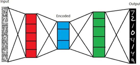
Autoencoders are an unsupervised learning method in which the developer creates a neural network with the goal of recreating the input fed into the network as the output. In order to force the network to learn attributes found in the data and not simply saving the input and feeding it unchanged as at the output, we create a bottleneck between the input and output layer making the network non-linear. A bottleneck meaning that the layers between the input and output contain less data points forcing a compression or encoding of the data to occur. To learn to accurately recreate the data the Autoencoder needs to feature a loss function in order to compare the recreated data to the original and calculate the error between the two. This error value is then used to update the weights in the Autoencoder to make a better prediction the next time. Autoencoders stand out amongst other neural network methods due to that they can learn almost any type of data automatically, they do not require labels on the data and that they are a lossy algorithm. With the goal of the Autoencoders learning process being to recreate the data no labels are needed. Because the data is compressed between the input and output layers it is inevitable that some of the data will be lost along the way [19]. Figure 2 displayed below shows the structure of an Autoencoder, with the encoding layers to the left, encoded representation in the middle, followed by the decoder. The type of Autoencoder visualized is a denoising Autoencoder.

Figure 2. Denoising autoencoder structure, encoding layers to the left, followed by the coded representation and finally the decoder. Based on:

https://laptrinhx.com/denoising-autoencoders-with-keras-tensorflow-and-deep-learning-4086106458/

10

(12)

The type of layers used in the Autoencoder plays an important role for the type of data the Autoencoder is working with. Because the EEG data is a sequential form of data, like audio and video, a layer that can handle sequential data is needed. This version of neural network is known as a Recurrent Neural Network (RNN). This kind of network is designed for data to persist between each input sequence. The type of RNN used in this thesis is Long Short Term Memory networks (LSTM), specifically designed to remember information for long term dependencies. While the most basic RNN would feature one module with data from the previous step a LSTM node has four modules to achieve long term dependencies. A forget gate, input gate, activation function, and output gate. The forget gate as the name states decides which information the LSTM node will get rid of during the current cycle. Input gate decides which values are to be updated using the sigmoid activation function. Finally the output gate decides which data will be forwarded to the next step of the network using a tanh activation function [20]. Figure 3 displays the components of a LSTM node. From left to right they are the following; input gate, forget gate, activation function and output gate.

Figure 3, LSTM components. Based on: https://colah.github.io/posts/2015-08-Understanding-LSTMs/

11

(13)

2.2.4 Support Vector Machine

Support Vector Machine is a comparatively simple machine learning algorithm that produces high accuracy prediction for the amount of resources consumed. SVM can be used for both classification and regression, in this paper it will only be used for classification. It can be used for any number of features to classify and will operate in the Nth dimensional space where N is the number of features. In this study it will perform binary classification thus operating only in 2D as shown by figure 4 [21]. The SVM works by attempting to find the optimal hyperplane that distinctively separates the data points, thus classifying them. To successfully separate the two classes any number of hyperplanes can be drawn. During training the SVM attempts to find the hyperplane that results in the greatest distance between the two classes to act as reinforcement when classifying future data points. The hyperplane is what decides which class each data point is assigned, if the data point falls on one side of the hyperplane it is given one classification and if it falls on the other it is given the other. The data points that lie the closest between the two classes are known as the support vectors, in figure 4 these are the circled dots. The hyperplane is drawn in the middle of the classes with the help of the support vectors [21].

Figure 4, Visualization of a support vector machine. The hyperplane is visualised by the solid line and the support vectors are visualised by the dotted lines.

Based on: https://scikit-learn.org/stable/modules/svm.html

12

(14)

2.2.5 Linear Regression

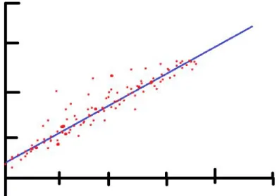
Linear Regression is one of the most basic regression algorithms in machine learning. Regression algorithms are used to forecast and find a relationship of cause and effect between variables. Linear Regression can be used when there is only one independent variable and the goal is to find a linear relationship between this independent variable x and the dependent variable y. The blue line in figure 5 is drawn to fit a straight line as best as possible along the given data points [22].

The version of Linear Regression used in the study is known as Ordinary Least Squared error. It is done with the following formula y_i= α + βx_i+ ε_iin the simplest terms we can imagine α being the value where the line intersects the y-axis. While is the angle of the line relative to the x-axis andβ ε being the error rate, in other words, the distance the data point has from the line. The model will attempt to find the correct parameters to minimize the error term to maximum effect. It should be noted that the error term is squared to ensure errors of both positive and negative values have the same impact on the algorithm [23].

Figure 5. Visualising linear regression. The algorithm attempts to draw a line alongside the dots representing the data points. Based on: https://en.wikipedia.org/wiki/Linear_regression

13

(15)

2.2.6 Logistic Regression

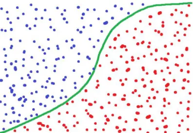
Logistic Regression (LR) is a predictive algorithm, just like Linear regression. LR differs from Linear regression by requiring the dependent variable to be categorical, since LR can perform both regression analysis and classification. LR is compatible with both binary and multi-class classification, binary classification being classification between two values, such as one or zero. Multi-class classification is classifying with three or more classes.

Logistic Regression can be visualized with a sigmoid function with a horizontal line classifying the decision bound. The algorithm classifies by feeding the data point(s) as input along with weights as input to a Sigmoid function. Then inferring from that result what class the data point belongs to. In our case this will look the same as the classification for Linear Regression, values above 0.5 are classified as 1 and vice versa. The predicted value can be seen as more or less confident concerning how close it is to the decision bound. With values going toward positive or negative infinity being very confident and values close to 0.5 as being very unconfident. Figure 6 visualizes the classification of two classes [24].

Figure 6. Visualising logistic regression classifying two types of samples. Based on:

https://www.datasciencecentral.com/profiles/blogs/why-logistic-regression-should-be-the-last-thing-yo u-learn-when-b

14

(16)

2.2.7 Random Forest

Random Forest gets its name from decision trees. A Random Forest contains numerous random decision trees where the predicted outcome of the forest is the most commonly guessed feature among the different trees. Each decision tree looks for randomly selected characteristics in the data and goes deeper into sub-branches to a predetermined maximum depth where they classify the given dataset from one of the possible classifications. Random Forests have the benefit that any random errors in guessing what feature is the correct answer are ignored since the majority vote wins. Decision trees are built on trying to find the most common feature in the data set the tree is given. It keeps dividing the data into more specific features for every branch taken until the tree is done guessing. TowardsDataScience used the example of separating a series of numbers with two different colors and some numbers being underlined. In the first branch, we separate the numbers by color, blue, and red. In the next branch, we separate the numbers from those who are underlined and those who are not underlined [25]. Random Forests build on using this idea but in scale. To achieve the random part, both the features to separate by and the data is random. The features are randomly generated but the data is different for each tree with the use of bagging. The total data set could be a series of numbers between zero and ten, but we will not give the whole data set to each tree but rather a subset of the data. This combined with random features to look for and letting the majority vote carry the final guess makes Random Forest a good choice for data classification. Figure 7 provides a visualization of a Random Forest classifier.

Figure 7. Visualizing a Random Forest classifier of n number of trees.

Based on: https://community.tibco.com/wiki/random-forest-template-tibco-spotfire

15

(17)

3. Related Work

3.1 Feature Extraction

Feature selection and classification of the specific EEG data used in this study have been used in a previous study published in 2019, “Feature Selection of EEG Oscillatory Activity Related to Motor Imagery Using a Hierarchical Genetic Algorithm” [26]. That study used a Hierarchical Genetic Algorithm for feature selection instead of Autoencoders. For the classification the study implemented a Support Vector Machine with a linear kernel, this study also implements the Support Vector Machine for classification. It does not however use the linear kernel as the previous study did. Providing a similar classification algorithm but not identical.

Further research using the same data with one of the most widely used genetic algorithms, NSGA-II was published in June of 2020 by the same main author that wrote the study using a Hierarchical Genetic Algorithm [26]. The new study is titled “Impact of NSGA-II Objectives on EEG Feature Selection Related to Motor Imagery” [27]. NSGA-II is used in union with a hierarchical individual representation to determine which EEG channels are irrelevant for motor imagery and are to be excluded. Results using the same EEG data as this thesis and the previous study, show that using k-Nearest Neighbours together with Pearson’s Correlation as the objective functions resulted in improved classification accuracy when compared to other combinations. Classification accuracy being improved from 69% to 73%. Other methods used by the study to maximize feature reduction, such as Linear Discriminant Analysis resulted in lower classification accuracy.

Similar research has been performed in predicting patient response to anticancer drugs. A Chinese study named “Autoencoder Based Feature Selection Method for Classification of Anticancer Drug Response” from 2019 [7]. Used Autoencoders for feature selection to find genetic biomarkers in individuals using two datasets. Genomics of Drug Sensitivity in Cancer from the Cancer Genome Project and Cancer Cell Line Encyclopedia. For the classification, the study used the Random Forest algorithm, one of the classification algorithms used by this study as well. The study had results showing over 70% accuracy for 59 out of the 98 tested drugs.

The Huazhong University of Science and Technology in Wuhan, China, published a study in late october 2020 studying the use of a LSTM Autoencoder to detect anomalies in power plant equipment. Implementing a LSTM based Autoencoder network to learn a normal behaviour model of the equipment of the powerplant. Once the model had been learned by the network it attempted to perform early detection of abnormalities in the equipment in real time. The results of the study showed that the normal behaviour model that predicts the patterns of the equipment had excellent accuracy and error terms as low as 0.026 for the training data. 0.035 for the test data, using mean square error. The researchers claim that the proposed framework could effectively be used for early detection of abnormalities [8].

A croatian study from 2017 used a combination of wavelet transforms, stacked Autoencoders and LSTMs for stock price prediction. Using the wavelet transforms to remove noise from historical price data of the stock. Secondly, stacked Autoencoders were applied to create high-level features for prediction of the future stock price. Finally the LSTMs were fed the features created by the Autoencoders to forecast the next day closing price of the stock. The study performed this method on six different market indexes to evaluate the performance of the model. Stating the results show the proposed model outperforms similar models in both accuracy of predictions as well as profitability [9].

16

(18)

A 2020 study from Cornell University trained a variational autoencoder with a new constrained loss function to generate better suited features to improve the performance of EEG based speech recognition systems. The study demonstrates that both continuous and isolated speech recognition systems were successfully trained and tested on EEG features that the variational autoencoder created, and that results were improved with this model. The result was demonstrated on a limited vocabulary of 30 sentences in English for continuous speech and 2 sentences for isolated speech, as well in English [10].

17

(19)

3.2 Classification

In 2015 “Feature learning from incomplete EEG with denoising autoencoder” [28] was published in ScienceDirect. The study implemented a denoising Autoencoder for feature classification of incomplete EEG signals. Using the Lomb-Scargle periodogram, an algorithm that is used to characterize periodic signals from unequally sampled data. This was used to estimate the incomplete EEG data and then run through the denoising Autoencoder. With the authors stating the method can decode incomplete EEG data successfully to good effect.

“A Long Short-Term Memory Autoencoder Approach for EEG Motor Imagery Classification” [11] published in early 2020 performed similar research on feature selection and classification on EEG data in regards to MI on the left- or right-hand movements. Using a highly similar approach as this study with LSTM autoencoder the study achieved 81% accuracy as a total average with the best subject scoring 96% accuracy.

Classification of EEG signals to distinguish between focal and nonfocal seizures in patients with epilepsy is crucial before resorting to surgery. A study from Abu Dhabi proposed to automate this using a deep learning approach with a LSTM algorithm to perform the classification between focal and nonfocal seizures. The study made use of publicly available data from the Bern-Barcelona EEG database, where they collected 7500 pairs of x and y EEG channels. Each signal was then manually classified as either focal or nonfocal by two certified electroencephalographers and neurologists. Classification was done using k-fold cross validation of 4, 6 and 10 fold. The algorithm developed achieved an overall accuracy of 99.6% when using 10-fold cross-validation [29].

Research in automatic seizure detection using EEG data and a denoising sparse autoencoder from the Shandong University in China achieved effective accuracy. The denoising sparse autoencoder is an unsupervised neural network which the researchers state can closest learn the representation of the data, and the sparsity constraint forces the EEG data to be more compressed in order to increase efficiency of the network. To help enhance the robustness of the system the researchers corrupted parts of the input data, in order to make the system suitable for non stationary EEG readings. A logistic regression classifier was used for classification of the data. The effective results of the study were 100% average sensitivity, 100% in specificity and 100% in recognition [30].

Semisupervised text classification has been attempted using a semi-supervised sequential variational autoencoder by researchers at the Chinese National Natural Science Foundation. The researchers performed the study by treating the category label of the unlabeled data or text as latent variable. Creating a model to maximize varitational evidence lower bound data. Which derives the underlying label for the unlabeled data. Using this model together with two types of decoders proved that experimental results show that the method vastly improved in classification accuracy compared to previous approaches and methods [31].

A turkish study from 2018 made attempts to perform automatic diagnosis of cervical cancer, using a softmax classification with a stacked autoencoder. They used a dataset containing 668 samples from the UCI database for the study. First applying the stacked autoencoder on the raw data, to reduce the dimensions of the data. Then using the reduced dataset for training with the softmax layer. This is the first study applying softmax classification with a stacked autoencoder to the UCI dataset, which performed better than previous methods. The results showed an accuracy of 97.8% correct classifications using softmax classification [32].

18

(20)

4. Problem Formulation

The first goal of this thesis is to establish whether Autoencoders can prove to be an effective tool to classify EEG signals related to the motor functions of the human body. This will be done by training an Autoencoder to extract features in patient EEG data. Once the features generated allow the Autoencoder to recreate the input to a high degree of accuracy they will be used for classification in the second experiment. The purpose is to potentially and hopefully help patients going through the rehab process after a stroke or similar accident that may have affected their motor functions. Providing an automated way to determine if the patient is performing their rehab exercises correctly, or to help isolate if the motor control issue is in the head or in the arm could help with rehabilitation by helping to faster diagnose the issue. The second goal of the study is to successfully classify the data to a reasonable degree of certainty, that it would prove useful for rehabilitation workers or others benefiting from EEG data classification. If possible the study will attempt to answer the following. How long does the Autoencoder have to train to reach this level of certainty? What the highest degree of certainty the study can achieve, as well as which classification method is best suited for classifying the problem. Leading to the questions the study will attempt to answer.

Research question 1: How to extract features from EEG signals using Autoencoders?

Research question 2: _{Which supervised machine learning algorithm identifies as the best}

classification based on the features generated by the Autoencoder?

19

(21)

5. Method

The chosen research method to answer the research questions was a set of experiments. First to evaluate the Autoencoders ability to construct features and reconstruct the input data using different combinations for the dimensions of both the input layer and encoding layer. To evaluate how the different variables would affect the loss rate for the recreation of the data. This experiment was performed using the Keras Machine Learning library to create the Autoencoder.

The second experiment was conducted to classify the features created by the Autoencoder from the first experiment. With the goal to answer the research questions “ _{How to extract features from EEG} signals using Autoencoders?” and _{“Which supervised machine learning algorithm identifies as the} best classification based on the features generated by the Autoencoder?” . This experiment was done by performing multiple sub experiments, by evaluating the accuracy of multiple machine learning classification methods. Main goal of this experiment was to evaluate the accuracy of the different classification algorithms. As well as answering how fast the different classification methods could classify the data. Since we had a limited number of samples of 240 for each subject, the classification was done with 5-fold cross validation to maximize the test data to the highest degree possible. The classification methods chosen to be used in the study came from the result of a literature review.

20

(22)

6. Ethical and Societal Considerations

The EEG signal data is personal data that is confidential, but this data is anonymized and can not be related back to the individual it originated from. Since the data is already anonymized no action is required to keep confidentiality. The hope is that the result of this study can help further future research in developing rehabilitation methods for stroke patients as well as possible insight on how to process EEG data for the next generation of prosthetics. The data was kept on a local harddrive throughout the experiment and excluded from all version control software used during development. The data used was provided to me by my thesis supervisor and thus I do not have access to any information sheet or consent form signed by the participants. For further information regarding the specific details of the EEG data see references [26] [27].

21

(23)

7. Implementation

7.1 Dataset description

The data was collected from 5 healthy individuals with a mean standard age of 3.5 3 ± 12.4 . The data was recorded while the subjects were performing a task of motor imagery and motor execution, only the motor imagery data was used for this project. For the motor imagery data the subjects were tasked with imagining either opening or closing their right hand whilst looking at a computer monitor, telling them when to perform the action. Each time the subject was meant to perform the action they received both a visual and auditory instruction for 4 seconds. This was followed by a focus window for 2 seconds, after which the subject was meant to perform the task. The subjects were then given 4 seconds to perform the task once, with their eyes open. How the experiment was planned and specifics such as why the focus window was 2 seconds long I can not answer since I did not partake in recording the data.Only healthy subjects were included in this study since this is a pre-study using healthy subjects as a baseline measurement. Subjects with motor difficulties such as stroke patients are being considered for future work. More information can be found in reference [27].

The motor imagery data was recorded using 64 Active Ag/AgCI electrodes. 42 channels were selected to be saved from the EEG recording: AFz, Fz, F1-4, FCz, FC1-6, Cz, C1-6, CPz,CP1-6, Pz, P1-6, POz, PO3-4, PO7-8, Oz, O1-2. Each subject had 240 samples recorded with a sampling of 1000 Hz, 120 of which were motor imagery.

7.2 Splitting and generating the data

Each sample from the original EEG dataset has the shape of 201 timesteps, each containing 42 channels, with each channel containing 30 frequencies. There were 240 samples containing 201 timesteps for each subject used in the study. Before use, the data had to be reformatted from its current form before it could be used to train the Autoencoder. The type of network that was going to be used works with sequential data so the timesteps could remain in the final form. The channels and frequencies however, had to be flattened into just one dimension when fed into the network. Finally, only a portion of the timesteps in the original data would be used for training and classifying. The majority of the timesteps would serve no purpose. Half of the samples did not contain any timesteps where the patient either imagined or actually closed their fist, those samples were filtered out. Additionally we only wanted the timesteps where the patient were actively performing the exercise, and an equal amount of timesteps where the patient is resting as a control case for brain activity that does not correlate to hand movement. Timesteps 0 to 40 served as the control data where the patient rested. Time step 60 to 100 were the steps where the patient performed the exercise. Then the order in which the different samples were used was scrambled by the Autoencoder. The remaining timesteps in the dataset were discarded.

The new dataset containing only rest and exercise timesteps was then flattened from 42 channels each containing 30 frequencies into one dimension containing just 1260 frequencies per timestep. The sequences were now 40 timesteps long instead of the original 201, and the number of samples per subject was still 240. No additional preprocessing was performed on the EEG data such as removing artifacts, more information regarding preprocessing can be found in references [26] [27].

22

(24)

7.3 Training the Autoencoder

The Autoencoder is made up of multiple layers, the first being an LSTM as the input, a dense layer for encoding, and a RepeatVector to repeat the signal from the dense to make it sequential and fit into the final LSTM decoder. The input and output of the whole network are 1260 neurons since that is the number of features the original data contains, and during training the goal is to recreate the data. To understand how well the Autoencoders can encode the data the feature count on both the Dense layer and the output of the first LSTM layer were varied to generate a large pool of data for classification. The feature count of the Dense layer changed between 1, 2, 5, 10, 50, 100, 200, 500, and 1260 neurons. The LSTM output feature count had the following values, 10, 50, 100, 200, and 500. The changes in the feature count were performed for each count of LSTM output feature count, for each subject. In order to maximize both the training data as well as the validation data we used five-fold cross validation. Generating features to classify on for each fold, and using the mean classification result. The most basic Recurrent Neural Network will only feature one repeat module, the module that stores context from previous time steps. LSTMs on the other hand feature four modules, designed to memorize data patterns long term. Thus an LSTM Neural Network was the chosen network type for the Autoencoder. Because the EEG data is a sequence of time steps of recorded brain activity a Neural Network that would be able to treat the input as a connected sequence was needed. A standard Artificial Neural Network would not suffice in this case since it does not recognize the input as a connected sequence but as completely different separate inputs. The goal for the Autoencoder was to find features in the data and recreate the input. Thus the design of the Autoencoder network had an LSTM layer as the input, followed by a Dense layer, with a repeat vector that then fed to a final LSTM output layer that attempted to recreate the original input.

A Dense layer is the most standardized layer type in Keras. It is a common deeply connected neural network layer. Taking input from the previous layer and applying its activation function, Sigmoid in the case of this study. On all neurons, then feeding the results forward to the next layer. The Dense layer was supplemented with a RepeatVector to fit with the final LSTM layer. Since a Dense layer is not a sequential layer as an LSTM layer is, it only feeds forward one output step rather than a stream of data. The RepeatVector solves this by repeating the output from the Dense layer into a stream for the final decoder LSTM layer.

The goal for the Autoencoder was to recreate the data to its best ability, thus we did not measure the accuracy of the Autoencoder but rather the Mean Square Error. The lower the MSE the closer the recreated data is to the original.

23

(25)

7.4 Classifying the encoded data

To get a measurement for the performance of the Autoencoder the goal is to measure the accuracy by classifying the different encoded samples. This was done by using the following set of different Machine Learning classification methods, Artificial Neural Network, Support Vector Machine, Linear Regression, Logistic Regression, and Random Forest.

The Artificial Neural Network was built using the Keras library, featuring just two Dense layers. With the first layer being the encoding layer and the second layer being the decoding layer. The encoding layer had 10 features as an output dimension that fed into the decoding layer with just one output feature. Both Dense layers used Sigmoid as their activation function. Since the classification is being done in binary, either hand movement or no hand movement, only one neuron with the value 1 or 0 was needed. This process is repeated five times for the specific subject with the specific neuron count with only the only thing changing being the partition of the data that acts as the test data. Then calculating the average accuracy and writing it to file. The ANN was trained for 100 epochs, using a batch size of 16. With binary cross entropy as the loss function and adam as optimizer.

The SVM was written using the Scikit-learn library. Scikit-learn was chosen for featuring all of the different classification algorithms needed, Artificial Neural Network being the exception. As well as for the code needed to change between the different classification algorithms was minimal, allowing for the majority of the code only being needed to be written once. The SVM was created using the

make_pipeline() function from Scikit learn, using the standard scaler, and Support Vector Classifier

with gamma set to ‘scale’.

Linear Regression as the name states is a regression algorithm and not a classification algorithm. Thus it computes continuous numerical values and does not perform classification as SVM does. Therefore we had to manually classify all results the algorithm predicted. This was done by rounding up all values above 0.5 to 1 and all values below 0.5 to 0, giving us a binary classification. The regression algorithm was created by calling Scikit-learn LinearRegression() function and then fitting the training data.

Logistic Regression just as Linear is a regression algorithm, it does however feature a classifier built in and there was not a need to program our own classifier for the predictions made by the regression algorithm. The algorithm was created by calling Scikit-learn LogisticRegression() and featured the standard 100 iterations of scikit-learn for the solvers to converge.

The random forest classifier was purposely limited to a max depth of 4 in order to ensure the execution time was not all too long compared to the other classification algorithms. The forest was created by calling RandomForestClassifier() and featured the standard number of 100 estimators for scikit-learn. As previously stated all classification algorithms were executed five times for each training session for the specified neuron-, featurecount and subject. With the average accuracy being saved.

The hyperparameters were left to default for the majority of the classification algorithms, since I had little to no experience on working with these classification algorithms prior to this thesis. Prioritizing time on other aspects of the research instead. Mostly due to the classification serving only as a metric of how accurately the features extracted by the Autoencoder could be classified.

7.5 Hardware and software specifications

All of the simulations performed for the implementation was run on a computer using the following hardware.

CPU: AMD Ryzen 7 2700X overclocked to 4.1 GHz GPU: Nvidia GeForce GTX 970

RAM: 16 GB DDR4 3000MHz

24

(26)

The following software versions were used. Python: 3.7 Keras: 2.4.3 Scikit-learn: 0.23.2

8. Results

This section will analyze and compare the results from the different classification methods explained in the previous chapter. Starting off with comparing the loss for different combinations of features and neurons when training the Autoencoder.

8.1 Feature generation with Autoencoders

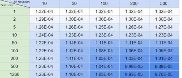
Increasing the number of features and neurons in a network should generally improve accuracy of a network, since you are giving the network more data to work with. Table 1 displays the average mean square error for the final epoch for all subjects during the training of the Autoencoder. The improvements are fairly linear when increasing both feature count and neuron count, slightly angled to being more influenced by the feature count than the neuron count.

The MSE stayed around 1e-04, with values somewhere around 1.3e-04 for lower feature counts and just under 1e-04 for higher feature counts on the Dense layer. After roughly 100 epochs the MSE stabilized and therefore, chose 100 epochs for training the Autoenocer on all different feature counts. When the training was complete the original data was processed through the encoding layers one final time and then written to file, to be used for classification.

Table 1. Average mean square error for all subjects for each feature and neuron count. Number of features in the left vertical column and number of Autoencoder neurons in the top horizontal columns.

25

(27)

8.2 Performance of different classification methods

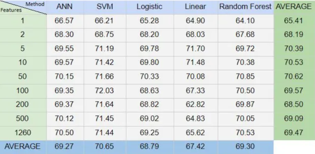
In order to compare different classification methods, all data was simulated using all pre-decided combinations of features and neurons. The results can be found in table 2. Values of each cell are the average for all neurons and all subjects given a specific feature count and classification method. Average on the bottom displays average for the column whilst average on the right displays the average for the row. The average accuracy across all feature counts and classification methods is 69.1% with a standard deviation of 2.25%. All classification methods had similar performance with a difference of roughly 3% between SVM the best performing algorithm, and Linear the worst performing algorithm. The difference is slightly greater for the different feature counts with 1 feature performing the worst and 50 features performing the best with a difference of just above 5.2%.

Table 2. Average accuracy for classification method over features for all neurons..

26

(28)

A comparison of how large influence the feature count respectively the neuron count has on the result can be found in table 3. Which displays the average result for all classification methods of all subjects given a specific number of features and neurons. The average on the bottom displays the average for the column whilst the average on the right displays the average for the row. From this table we can conclude that the feature count has a larger impact on the accuracy of the classification results than the neuron count from the Autoencoder does. The difference between the best performing feature count of 50 and worst performing feature count of 1 is 5.2% whilst the same for the neuron count only has a difference of less than 2.2%.

Table 3. Average accuracy for neurons over features for all classification methods.

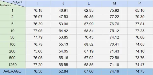
The different performance of the various subjects is compared in table 4. Which displays the classification result for each subject using the average for all classification methods and all neuron counts. Average on the bottom displays the average for the specific column or subject. The largest difference in accuracy is almost 24%, between subject I and J could indicate that MI may not be suitable for all patients that could benefit from it. It could also indicate that some patients need more training when performing motor imagery to achieve sufficient results.

Table 4. Average of all classification methods and neuron counts for each subject over all neurons.

27

(29)

The overall best performing subject was subject I using the Support Vector machine achieving a maximum accuracy of almost 83% with 200 features and 500 neurons. This is displayed by table 5. The accuracy improvements drastically slow down after 100 features and 100 neurons when the classification achieves 82% accuracy. Improving less than 1% when reaching the maximum accuracy of 82.9% at 200 features and 500 neurons.

Table 5. SVM accuracy for subject I for each feature and neuron count.

28

(30)

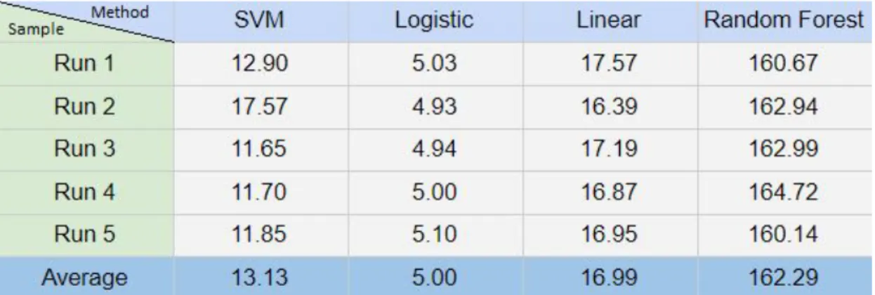
8.3 Execution time of the classification methods

The execution time is measured for training and classifying all 1225 training samples generated by the Autoencoder. The results are the sum of the total execution time for all samples and is measured in seconds. Artificial Neural Network was excluded from this list due to taking over 24 hours to train and classify the data. In a situation where speed is important it would not be a viable method and is therefore excluded from the list.

Table 6. Execution time for all classification methods with the exception for ANN. Measured in seconds.

The execution time of the different classification algorithms is compared in table 7 and 8. Table 7 displays the average time it takes to perform one classification of one sample after training is complete. Taken from 75 samples ranging from 5 features to 500 features to get an average for all feature counts. Table 8 is a conversion of the data from table 7 to how many samples are classified per second.

Table 7. Average time to classify one sample. Measured in seconds.

Table 8. Average number of samples classified per second.

29

EEG signals for motor imagery

ANN SVM Logistic Linear Random Forest

1.71E-03 3.42E-05 4.72E-06 5.00E-06 1.62E-04

ANN SVM Logistic Linear Random Forest

(31)

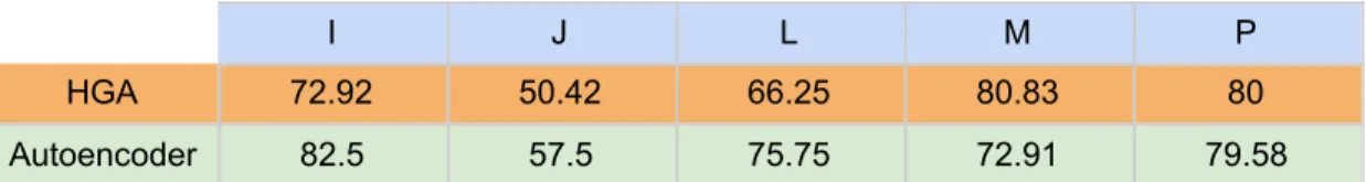
8.4 Comparison with Hierarchical Genetic Algorithm and NSGA-II

The subjects used in the study with a Hierarchical Genetic Algorithm (HGA) [26] were named subject A - F in the paper and contained one more subject than this study, which was removed before this study began. The subject labels from that study have been translated to match those used in this thesis. The HGA study used a SVM for classification of the features selected, the lowest number of features used in that study were 1260. Thus the result when using 1260 features were selected for comparison to this study in order to compare the result when using the same number of features. The results can be found in table 9 below. The Autoencoder achieves high classification accuracy overall with subject I at 82.5%, almost 10% higher accuracy compared to the HGA. The worst performing subject fared better with the Autoencoder as well, 57.5% compared to 50.42% for HGA. The results continue this trend for subject L with roughly a 9% lead for the Autoencoder. For the final two subjects, M and P the HGA provides better accuracy, at almost 8% higher for M and roughly 0.5% for P.

Table 9. A comparison of accuracy between HGA using 1260 features and a window size of 40, to the Autoencoder using 1260 features and 100 neurons for the dimension of the input layer.

The study using NSGA-II [27] used 6 subjects just as the HGA study did, the new study did however not provide results for each individual but rather the average result for a specific classification algorithm. Thus when comparing the result between this study and the NSGA-II it should be noted that this study features one less subject, which will have an impact on the result. The NSGA-II study featured 6 different classification algorithms, only one of which was also featured in this study, ANN. Therefore the average accuracy of ANN from both studies was chosen for a comparison, since that is the closest comparison possible of the result between the two studies.

NSGA-II has an average classification accuracy for ANN of 1.26% higher than the Autoencoder does, displayed in table 10. Whether the difference is due to the removed subject performing exceptionally well in NSGA-II or if it comes down to the algorithm itself is not possible to determine with the data available.

Table 10. Comparison of average Artificial Neural Network classification accuracy between NSGA-II and Autoencoder.

30

EEG signals for motor imagery

I J L M P

HGA 72.92 50.42 66.25 80.83 80

Autoencoder 82.5 57.5 75.75 72.91 79.58

NSGA-II 70.53

(32)

9. Discussion

The main objective of this study was to find out how well Autoencoders are suited for finding and creating features in the EEG data. A large part of that process is recreating the data inputted into the Autoencoders and evaluating if the factor of how aggressively the data is encoded will impact performance. For example 1260 features were used as a base line where no compression is performed, the Autoencoder outputs just as much data as it was fed. Whilst with 1 feature the data is compressed to 1/1260th of the original size. Table 1 visualizes how much the recreation of the data is improved by giving the Autoencoder more features to work with. Going from just 1 feature and 10 neurons to the maximum of 1260 features and 500 neurons improved the results by 26%. Moving from 1 feature to 50 features and 100 neurons improved the result by another 16%. For classification the results data loss from the Autoencoder do not seem to impact much, with average accuracy using 1 feature and 10 neurons being 65.7% and for 50 features and 100 neurons this only increases to 70.5%. Increasing the feature and neuron count from there to the maximum only improves accuracy by 0.l% further. The results indicate that while increasing feature count, neuron count and using better suited classification algorithms does improve the result. The variable that has the most impact on the results has shown to be the individual itself. A good example of this is table 4 that displays the average accuracy for specific individuals using specific feature counts. With only one feature for subject I the average accuracy is 76.19%, with only changing the parameter of subject from I to J the accuracy goes as low as 46.9%. An accuracy that is worse than a random coin toss. The best average accuracy achieved by Subject I was 77.79% at 50 features and performed the worst at 5 neurons reaching 76.3%. Subject J on the other hand peaks at 55.54% with 1260 neurons and has its worst performance with 46.9% with 1 neuron. The worst performance for Subject I had a 20.76% better accuracy than subject J’s best performing accuracy. Which goes to show that the most important factor is the subject itself in order to find appropriate features to classify on.

As stated earlier in the report the overall best performing classification function was the Support Machine Vector. It was the only classification method to achieve an average accuracy over 70% as displayed by table 2. The other classification methods were not far behind with ANN and Random Forest at 69%. 68% and 67% accuracy for the regression methods, Logistic and Linear.

When discussing performance it is often important to look at more than just one aspect. So far the report has only discussed the performance attribute of accuracy. Table 6 brings another attribute to light, execution time. If the idea is to use classification of EEG signals in real time as they are being sampled from the patient, speed will become an important factor. In such a case we might want to steer away from classification methods that can not keep up with the rate at which the data is sampled from the patient. Table 6 displays the total time it takes for the classification methods to train and classify the whole dataset. But if such an application was meant to work in real time it would first have to train the network and first when training of the classification algorithm is complete would you be able to classify in real time. Table 7 only displays the time it takes to classify one sample using the different algorithms. American Clinical Neurophysiology Society states in their guidelines that EEG data should be sampled at a minimum of 200 samples per second i.e. 200hz in order to prevent aliasing [33]. Considering that the slowest classifier ANN, classified 585 samples per second and Logistic and Linear regression classified over 200,000 per second. Using a pretrained network for live classification should not prove to be an issue, if a moderately powered computer is used.

The report set out to answer the question of “ _{How to extract features from EEG signals using} Autoencoders?” and there is no short answer to the question. The answer is that it varies depending on several factors. Both, how many features and neurons are used to create the features as well as which classification method was used and the most important factor is the subject. As mentioned previously, the results can vary between 76.19% and 46.9% accuracy by only switching subjects. At its best the classification can achieve 82.9% accuracy using 200 features and 500 neurons. Showing that more data is not always better since the accuracy drops by 2% when moving to 1260 features.

31

(33)

Answering the second research question “Which supervised machine learning algorithm identifies as the best classification based on the features generated by the Autoencoder? ” is a lot easier. If accuracy is the most important factor the answer is Support Vector Machine, for every subject SVM has the best average accuracy of all the different classification algorithms. There were a few cases where other algorithms performed better, but the difference there was less than 1% every time. An example of this is in table 2, when using 5 features Linear Regression had an accuracy of 71.7% and SVM had a classification accuracy of 71.19%, 0.51% less.

If hardware is limited and speed is of importance Logistic Regression or Linear Regression would perform better than SVM. Logistic Regression had an average classification result of 68.79%, 1.86% less than SVMs 70.65%. But LR classified 211705.82 samples per second, compared to SVM which classified 29281.99 samples per second, roughly 14% of the speed of Logistic Regression. Linear regression performed similarly to Logistic regression, only slightly slower with slightly lower accuracy.

32

(34)

10. Conclusions

This study trained Autoencoders to find features in EEG data. In order to answer the questions “ How to extract features from EEG signals using Autoencoders?_{” and “Which supervised machine learning} algorithm identifies as the best classification based on the features generated by the Autoencoder?” _.

The main goal of the study was to evaluate the performance of Autoencoders for finding and creating features using the EEG data. The performance of these features were determined by classification using a variation of different classification methods. Artificial Neural Network, Support Vector Machine, Linear- and Logistic regression and Random Forest. In order to find which combination of output features and output neurons worked the best the training featured a wide selection of both features and neurons varying between 1 - 1260 and 10 - 500 respectively. The best performing classification method in terms of accuracy proved to be the Support Vector Machine. If classification speed is more important Logistic Regression performed the best, SVM had 1.86% higher accuracy but only 14% of the speed that Logistic Regression had.

The best performing subject was subject I, and the worst performing was J. The difference in average accuracy between these two was 76.58% and 52.84%. This difference was greater than changing any combination of classification method, feature and neuron count, showing that the accuracy of the results is heavily dependent on the subject. The best combination of features and neuron proved to be 200 features and 500 neurons. Increasing the number of features to the maximum lowered the accuracy by 2%. 500 neurons was the highest that was simulated, all neuron counts less than 500 had worse performance. The global average accuracy for all classifications done with the SVM achieved 70.6% across all subjects and combinations of features and neurons.

33

Training Autoencoders for feature extraction of EEG signals for motor imagery

M

​

​

S

​

​

​

​

​

​

V

​

​

Examensarbete för kandidatexamen i datavetenskap - 15 hp

T

​

RAINING

​

A

​

UTOENCODERS

​

​

FOR

​

​

FEATURE

EXTRACTION

​

​

OF

​

EEG

​

SIGNALS

​

​

FOR

​

​

MOTOR

IMAGERY

Casper Wahl

cwl17001

​@student.mdh.se

Examiner:

Mobyen Uddin Ahmed

Mälardalen University, Västerås, Sweden

Supervisor: Miguel León Ortiz

Abstract

List of Figures

List of Tables

List of Abbreviations

1. Introduction

2. Background

2.1 Motor Imagery

2.2 Machine Learning

igmoid(x)

s

=

3. Related Work

3.1 Feature Extraction

3.2 Classification

4. Problem Formulation

5. Method

6. Ethical and Societal Considerations

7. Implementation

7.1 Dataset description

7.2 Splitting and generating the data

7.3

​

Training the Autoencoder

7.4

​

Classifying the encoded data

7.5 Hardware and software specifications

8. Results

8.1 Feature generation with Autoencoders

8.2 Performance of different classification methods

_{@student.mdh.se}