https://doi.org/10.1051/0004-6361/202038909 c ESO 2020
Astronomy
&
Astrophysics
Theoretical investigation of oscillator strengths and lifetimes in
Ti ii
?
W. Li
1, H. Hartman
1, K. Wang
2, and P. Jönsson
11 Department of Materials Science and Applied Mathematics, Malmö University, 20506 Malmö, Sweden e-mail: wenxian.li@mau.se
2 Hebei Key Lab of Optic-electronic Information and Materials, The College of Physics Science and Technology, Hebei University, Baoding 071002, PR China
Received 13 July 2020/ Accepted 27 September 2020
ABSTRACT
Aims.Accurate atomic data for Ti
ii
are essential for abundance analyses in astronomical objects. The aim of this work is to provide accurate and extensive results of oscillator strengths and lifetimes for Tiii
.Methods. The multiconfiguration Dirac–Hartree–Fock and relativistic configuration interaction (RCI) methods, which are imple-mented in the general-purpose relativistic atomic structure package GRASP2018, were used in the present work. In the final RCI calculations, the transverse-photon (Breit) interaction, the vacuum polarisation, and the self-energy corrections were included. Results.Energy levels and transition data were calculated for the 99 lowest states in Ti
ii
. Calculated excitation energies are found to be in good agreement with experimental data from the Atomic Spectra Database of the National Institute of Standards and Tech-nology based on the study by Huldt et al. Lifetimes and transition data, for example, line strengths, weighted oscillator strengths, and transition probabilities for radiative electric dipole (E1), magnetic dipole (M1), and electric quadrupole (E2) transitions, are given and extensively compared with the results from previous calculations and measurements, when available. The present theoretical results of the oscillator strengths are, overall, in better agreement with values from the experiments than the other theoretical predictions. The computed lifetimes of the odd states are in excellent agreement with the measured lifetimes. Finally, we suggest a relabelling of the 3d2(1 2D)4p y 2Do 3/2and z 2Po 3/2levels.Key words. atomic data
1. Introduction
Iron-group elements have high cosmic abundances and display, due to their complex atomic structure, rich spectra in astronomi-cal objects. Titanium is among the lighter elements in this group and is identified as an α-element that is primarily produced by captures of He nuclei. Studies of metal-poor stars, aimed to probe early galactic chemical compositions, show correlations with abundances of scandium and vanadium and thus a common production route with the iron-group elements (Sneden et al. 2016).
Spectroscopic analyses of astronomical objects rely on accu-rate transition data for elemental abundances, which in turn are crucial input to stellar and galactic evolution modelling. Data that are needed include wavelengths and oscillator strengths as well as hyperfine structure. The current paper addresses this important need.
We note that Ti
ii
is one of the most abundant ions and its lines are found in the ultraviolet, visible, and near-infrared spec-tra of B, A, and F stars, for example. Furthermore, its parity forbidden nebular lines are found in stellar winds (Ryde 2009;Cowan et al. 2020;Hartman et al. 2004).
The energy levels of Ti
ii
presented in the Atomic Spectra Database (ASD) of the National Institute of Standards and Tech-nology (NIST; seeKramida et al. 2019) were compiled bySugar ? Full Table 3 is only available at the CDS via anonymous ftptocdsarc.u-strasbg.fr(130.79.128.5) or viahttp://cdsarc.
u-strasbg.fr/viz-bin/cat/J/A+A/643/A156
& Corliss(1985) andSaloman(2012) based on the results from
Huldt et al. (1982). The observed spectral lines of Ti
ii
were compiled from sources of Huldt et al. (1982), Allende Prieto & Garcia Lopez(1998),Pickering et al. (2001), andAldenius(2009) for electric dipole (E1) transitions and ofHartman et al.
(2004,2005) andBautista et al.(2006) for magnetic dipole (M1) and electric quadrupole (E2) transitions.
There are a number of experimental and theoretical studies of lifetimes and oscillator strengths of the Ti
ii
ion. The sources adopted in the compilation by the NIST ASD are summarised in Table1, and they include those ofRoberts et al.(1973,1975),Wolnik & Berthel(1973),Danzmann & Kock (1980),Kostyk & Orlova(1983), Pickering et al.(2001), Wiese et al.(2001),
Morton(2003),Hartman et al.(2005), andDeb et al.(2008). On the experimental side, a number of studies of lifetimes have been presented in the literature. Within the FERRUM project, Hartman et al. (2003) reported measurements of the long lifetime of the 3d2(3P)4s4P
5/2level in Ti
ii,
using the laser probing technique (LPT) (Lidberg et al. 1999) at the CRYRING storage ring (Abrahamsson et al. 1993). This measurement, how-ever, resulted in a lifetime (28 ± 10 s) more than a factor of 2 longer than the theoretical estimate. The large uncertainty was due to the systematic effect of repopulation. Later on, within the same project,Hartman et al. (2005) extended the work on the measurement of lifetimes of other four metastable levels and determined the absolute transition probabilities for eight forbid-den transitions originating from the levels 3d4s2 2D3/2,5/2, using a combination of laboratory and astrophysical measurements.Table 1. Summary of previous works on oscillator strengths and lifetimes in Ti II.
NIST database collection on oscillator strengths
Roberts et al.(1973,1975) exp. Beam-foil+ stabilised arcs
Wolnik & Berthel(1973) exp. Shock tubes
Hartman et al.(2005) exp. LPT+ astrophysical BF
Danzmann & Kock(1980) exp. Combined hook
Kostyk & Orlova(1983) exp. Solar spectra
Pickering et al.(2001,2002) exp. LIF+ FTS
Wiese et al.(2001) exp. HSAS
Morton(2003,2004) Compilation
Deb et al.(2008) theo. CIV3
Other works on oscillator strengths
Blackwell et al.(1982) exp. Oxford furnace
Thevenin(1989) exp. Solar spectra
Savanov et al.(1990) Compilation
Bizzarri et al.(1993) exp. LIF+ FTS
Luke(1999) theo. CI
Kurucz(2017) theo. Semi-empirical
Wood et al.(2013) exp. LIF+ FTS
Ruczkowski et al.(2014) theo. Semi-empirical
Lundberg et al.(2016) exp. & theo. LIF+ FTS + HFR Other works on lifetimes
Roberts et al.(1973) exp. Beam-foil
Kwiatkowski et al.(1985) exp. LIF
Gosselin et al.(1987) exp. Beam-laser method
Bizzarri et al.(1993) exp. LIF
Langhans et al.(1995) exp. LIF
Hartman et al.(2003,2005) exp. LPT
Bautista et al.(2006) theo. AUTOSTRUCTURE
Palmeri et al.(2008) exp.& theo. LPT+ HFR
Deb et al.(2008) theo. CIV3
Lundberg et al.(2016) exp.& theo. LIF+ HFR
Ruczkowski et al.(2016) theo. Semi-empirical
Kurucz(2017) theo. Semi-empirical
Notes. BF: Branching fraction; LPT: Laser probing technique; LIF: Laser induced fluorescence; FTS: Fourier transform spectroscopy; HSAS: High sensitivity absorption spectroscopy; CI: Configuration Interaction; and HFR: Relativistic Hartree–Fock (HFR).
Lifetimes for metastable levels were measured using the LPT. Branching fractions from some of these levels were derived from HubbleSpace Telescope/STIS spectra of Eta Carinae. With the development of methods to eliminate the repopulation effects,
Palmeri et al.(2008) re-measured the lifetime of 3d2(3P)4s4P5/2 using the same technique at CRYRING and they determined a shorter lifetime (16 ± 2 s).
A number of other authors have measured the lifetimes of short-lived Ti
ii
levels.Kwiatkowski et al.(1985),Bizzarri et al.(1993), andLanghans et al.(1995) performed the measurements using a laser-induced fluorescence (LIF) technique.Roberts et al.
(1973) determined some lifetimes of Ti
ii
levels using the beam-foil technique. These sources are also given in Table1.A frequently used method to determine transition proba-bilities or oscillator strengths for E1 transitions is to combine the lifetime for the upper level with branching fractions (BF). The lifetime can be measured using the LIF technique and the BF are determined from, for example, Fourier transform spec-troscopy (FTS) of a laboratory light source. This approach has been adopted byBizzarri et al. (1993),Pickering et al.(2001),
Wood et al.(2013), andLundberg et al.(2016) to derive absolute transitions probabilities.Wiese et al.(2001) measured the oscil-lator strengths for the Ti
ii
vacuum ultraviolet (VUV) resonancetransitions 3d4s4p 4F3/2o − 4d24s 4F3/2 at 191.0938 nm and 3d4s4p4Do
1/2− 4d 24s4F
3/2at 191.0609 nm, using the high sen-sitivity absorption spectroscopy (HSAS) experiment.
There are a few theoretical works presenting lifetimes or radiative transition rates for the complex system of Ti
ii
.Luke (1999) calculated transition rates for E1 transitions between the fine structure levels of the terms 3d24p {4Go,4Fo, 2Fo, 2Do, 4Do, 2Go} to the levels of the ground term 3d24s4F by using a configuration interaction (CI) method.Bautista et al.
(2006) carried out calculations of radiative transition rates and lifetimes for states belonging to the {3d24s, 3d3, 3d24p, 3d4s2} configurations using the AUTOSTRUCTURE package (Badnell 1986). However, some of the theoretical metastable lifetimes obtained significantly disagree with the earlier measurements (Hartman et al. 2003, 2005). Palmeri et al. (2008) presented theoretical lifetimes of 13 metastable levels, along with the transition probabilities for several decay channels from these metastable levels obtained from three pseudo-relativistic Hartree–Fock (HFR) calculations, that is, HFR(A), HFR(B), and HFR(C), using the Cowan code (Cowan 1981).Deb et al.
(2008) performed calculations of E2 and M1 transition proba-bilities among all 37 even parity levels, using the CIV3 code of
Hibbert (1975), together with a semi-empirical fine-tuning technique to reproduce the experimental energy separations.
More recently, calculations of oscillator strengths of radia-tive E1 transitions and lifetimes for odd-parity states have been performed using a semi-empirical method (Ruczkowski et al. 2014,2016).Lundberg et al.(2016) report oscillator strengths as well as lifetimes for highly excited states from laboratory measurements and calculations. The calculations were carried out using the HFR method of Cowan (1981), taking core-polarisation effects into account.
Extensive calculations of energy levels, oscillator strengths, and lifetimes in Ti
ii
were also carried out by Kurucz using the semi-empirical approach, and these data are available inKurucz(2017). The oscillator strengths fromKurucz(2017) for strong lines are well known to agree rather well with experimental val-ues, but for weak lines they are inevitably more uncertain.
In the present work, ab initio calculations were performed for the 99 (37 even and 62 odd) lowest states belonging to the even {3d24s, 3d3, 3d4s2} configurations and to the odd {3d24p, 3d4s4p} configurations in Ti
ii
. The calculations were performed based on the fully relativistic multiconfiguration Dirac–Hartree–Fock (MCDHF) and relativistic configuration interaction (RCI) methods, as implemented in the newest ver-sion of the general-purpose relativistic atomic structure package GRASP2018 (Froese Fischer et al. 2019). Energy levels as well as E1, M1, and E2 transition data were computed along with the corresponding lifetimes of these states.2. Multiconfiguration Dirac–Hartree–Fock approach
In the MCDHF method (Grant 2007;Froese Fischer et al. 2016), the atomic state functions (ASFs) used to describe the states of the atom are approximate eigenfunctions of the Dirac-Coulomb Hamiltonian given by HDC= N X i=1 [cαi·pi+ (βi− 1)c 2+ VN i ]+ N X i> j 1 ri j , (1)
where α and β are the 4 × 4 Dirac matrices, VN
i is the monopole part of the electron–nucleus Coulomb interaction, c is the speed of light in atomic units, pi ≡ −i∇ is the electron momentum operator, and ri j is the distance between electrons i and j. The ASFs (Ψ) are expanded over configuration state functions (CSFs, Φ): Ψ(γ PJMJ)= NCSF X i=1 ciΦ(γiPJ MJ). (2)
The CSFs are j j-coupled many-electron functions built from products of one-electron Dirac orbitals. As for the notation, J and M are the angular quantum numbers, P is parity, and γi spec-ifies the occupied subshells of the CSF with their complete angu-lar coupling tree information, including for instance the orbital occupancy, coupling scheme, and other quantum numbers nec-essary to uniquely describe the CSFs.
The radial parts of the Dirac orbitals together with the expansion coefficients ci of the CSFs are obtained in a rel-ativistic self-consistent field (SCF) procedure by solving the Dirac–Hartree–Fock radial equations and the configuration inter-action eigenvalue problem, resulting from applying the varia-tional principle on the statistically weighted energy funcvaria-tional of the targeted states with terms added in order to preserve the orthonormality of the one-electron orbitals. The angular integra-tions needed for the construction of the energy functional are
based on the second quantisation method in the coupled tenso-rial form (Gaigalas et al. 1997,2001).
Higher order interactions, such as the transverse photon interaction and quantum electrodynamic effects (vacuum polari-sation and self-energy), are added to the Dirac-Coulomb Hamil-tonian in subsequent RCI calculations (McKenzie et al. 1980). Keeping the radial components from the previous step fixed, the expansion coefficients ciof the CSFs for the targeted states are obtained by solving the configuration interaction eigenvalue problem.
The transition data (e.g. transition probabilities and weighted oscillator strengths) between two states γ0P0J0 and γPJ are expressed in terms of reduced matrix elements of the transition operator T (Grant 1974):
hΨ(γPJ) kTk Ψ(γ0P0J0)i=X j,k
cjc0khΦ(γjPJ) kTkΦ(γk0P
0J0)i. (3)
For E1 and E2 transitions, there are the following two forms of the transition operator: the Babushkin and Coulomb forms, which are equivalent to the length and the velocity form in the non-relativistic quantum mechanics. Babushkin and Coulomb gauges for the exact solutions of the Dirac-equation give the same value of the transition moment (Grant 1974).
3. Computational schemes
Calculations were performed in the extended optimal level (EOL) scheme (Dyall et al. 1989) for the weighted average of the even and odd parity states. These states belong to the {3d24s, 3d3, 3d4s2} even configurations and the {3d24p, 3d4s4p} odd configurations. From the initial calculations and analysis of the eigenvector compositions, we identified a number of configura-tions giving considerable contribuconfigura-tions to the total wave func-tions. Particularly, the two-electron excitation configurations {3p43d44s, 3p43d34s2, and 3p43d5} are of crucial importance to predict the correct order of the energy levels for even states. These important configurations, together with the target con-figurations, define what is known as the multireference (MR). The MR sets for the even and odd parities are presented in Table 2, which also displays the number of CSFs in the final even and odd state expansions distributed over the different J symmetries.
The CSF expansions were determined using the multireference-single-double (MR-SD) method, allowing single and double (SD) substitutions from configurations in the MR to orbitals in an active set (AS; Olsen et al. 1988; Sturesson et al. 2007; Froese Fischer et al. 2016). In the MCDHF cal-culations, no substitutions were allowed from the Ar-like core (1s22s22p63s23p6), which defines an inactive closed core. This means that only valence-valence (VV) electron correlation effects were taken into account in the MCDHF calculations. These calculations were followed by RCI calculations for an extended expansion, which was achieved by opening the 3s and 3p core shells for substitutions to include core-valence (CV) and core-core (CC) effects. In the RCI calculations, 1s22s22p6 was kept as an inactive closed core. The CV expansion was obtained by allowing SD substitutions from the valence orbitals and the 3s23p6core, with the restriction that there was one substitution at most from 3s23p6to the active set {8s, 8p, 8d, 8 f , 8g, 8h, 7i}. The inclusion of CC correlations in the calculations decreases the excitation energies significantly and they also have large effects on the energy separations. Considering the fact that the inclusion of CC correlations increases the number of
Table 2. Summary of the active space construction.
Parity MR Extended MR in RCI NCSFs
3 p63d3, 3p63d24s, 3p43d44s 3 p63d4s2, 3p63d4p2, 3p43d34s2 Even 3p64s24d, 3p63d4s4d, 3p43d5 14 089 101 3p63d4s5s, 3p63d24d, 3p63d4d2, 3p64s4d2, 3p64s4p2 3 p63d24 p, 3p63d4s4 p, 3p43d34s4p Odd 3p64s4p4d, 3p63d4s5p, 3p43d44p 15 573 967 3p63d4p4d, 3p64s24p, 3p64p4d2
Notes. MR: multireference, where the targeted configurations are labelled in boldface; and NCSFs: number of CSFs. Table 3. Transition data of E1, M1, and E2 transitions for Ti
ii
from the present calculations.Upper Lower EM ∆E λ S log(g f ) A
(cm−1) (Å) (s−1) 3d2(10S)4p2Po3/2 3d2(32F)4s4F3/2 E1 63375 1577.901 3.245E−07 −7.201 4.295E+01 3d2(10S)4p2Po 3/2 3d 2(3 2F)4s 4F 5/2 E1 63281 1580.248 1.274E−06 −6.607 1.679E+02 3d2(1 0S)4p 2Po 1/2 3d 2(3 2F)4s 4F 3/2 E1 63276 1580.356 8.055E−07 −6.807 2.120E+02 3d2(1 0S)4p 2Po 3/2 3d 3(4 3F) 4F 3/2 E1 62467 1600.836 7.410E−08 −7.849 9.371E+00 3d2(1 0S)4p 2Po 3/2 3d 3(4 3F) 4F 5/2 E1 62391 1602.785 3.301E−05 −5.200 4.161E+03 – – – – – – – –
Notes. Upper and lower states, transition type, wavenumber,∆E, wavelength, λ, line strength, S , weighted oscillator strength, log(g f ), transition probability, A, provided by the present calculations are shown in the table. Wavelength and wavenumber values are adjusted to match the level energy values in the NIST ASD (Kramida et al. 2019). Only the first five rows are shown; the full table is available at the CDS.
CSFs very rapidly, which is beyond the reach of the available computational resources, the CC expansion was obtained by allowing SD substitutions from both 3s and 3p shells to the active set {8s, 8p, 8d}. The MR set in the RCI calculations was extended to include additional important configurations. For these configurations, single substitutions from valence and core orbitals were allowed to the active orbital set {8s, 8p, 8d} and double substitutions to {4s, 4p, 4d}. The number of CSFs in the final even and odd state expansions are 14 089 101 and 15 573 967, respectively, and they are distributed over the different J symmetries.
4. Results and discussions
4.1. Energy levels
The energies and wave function composition in LS -coupling for the 99 (37 even and 62 odd) lowest states for Ti
ii
are given in Table A.1. In the calculations, the labelling of the eigenstates is determined by the LS J-coupled CSF with the largest coef-ficient in the expansion resulting from the transformation from j j-coupling to LS J-coupling using the method byGaigalas et al.(2017).
The accuracy of the wave functions from the present calcu-lation was evaluated by comparing the calculated energy lev-els with experimental data from Huldt et al. (1982) provided via the NIST ASD. In most cases, the differences of the com-puted energy levels compared to the experimental data are less than 1.0%. The largest disagreements are for the4Fstates in the
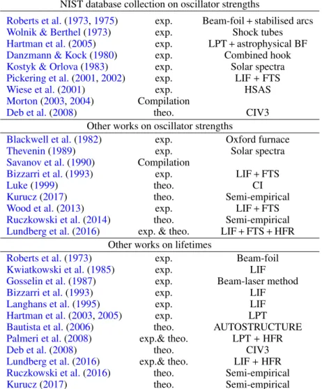
-4.5 -4.0 -3.5 -3.0 -2.5 -2.0 -1.5 -1.0 -0.5 0.0 0.5 log(gf)NIST -4.5 -4.0 -3.5 -3.0 -2.5 -2.0 -1.5 -1.0 -0.5 0.0 0.5 log( gf ) this work
Fig. 1.Comparison of log(g f ) values of the current study with the
val-ues available in the NIST ASD.
ground configuration 3d24s and the first excited configuration 3d3, and the differences are about 4%. The averaged uncertainty of computed energy spectra compared to NIST data is 1.06%.
In addition, the Landé g-factors for the 99 states in Ti
ii
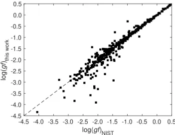
were derived from the wave function expansions. The results were col-lected and made available in a recent paper byLi et al.(2020), in which they provide a collection of theoretical Landé g-factors for ions of astrophysical interest.-1.0 -0.8 -0.6 -0.4 -0.2 0.0 0.2 0.4 log(gf)Blackwell -1.0 -0.8 -0.6 -0.4 -0.2 0.0 0.2 0.4 log( gf ) this work -1.0 -0.8 -0.6 -0.4 -0.2 0.0 0.2 0.4 log(gf)Blackwell -1.0 -0.8 -0.6 -0.4 -0.2 0.0 0.2 0.4 log( gf ) others Ruczkowski Lundberg Kurucz
Fig. 2.Comparison of the theoretical log(g f ) values to those published byBlackwell et al.(1982). Left panel: this work (black square). Right
panel:Ruczkowski et al.(2014) (red square);Lundberg et al.(2016) (blue circle); andKurucz(2017) (magenta triangle).
-3.5 -3.0 -2.5 -2.0 -1.5 -1.0 -0.5 0.0 0.5 log(gf)Bizzarri -3.5 -3.0 -2.5 -2.0 -1.5 -1.0 -0.5 0.0 0.5 log( gf )this work -3.5 -3.0 -2.5 -2.0 -1.5 -1.0 -0.5 0.0 0.5 log(gf)Bizzarri -3.5 -3.0 -2.5 -2.0 -1.5 -1.0 -0.5 0.0 0.5 log( gf ) others Ruczkowski Lundberg Kurucz
Fig. 3.Comparison of the theoretical log(g f ) values to those published byBizzarri et al.(1993). Left panel: this work (black square). Right panel:
Ruczkowski et al.(2014) (red square);Lundberg et al.(2016) (blue circle); andKurucz(2017) (magenta triangle).
4.2. Transition rates and oscillator strengths
Transition data, for example, wavenumbers, wavelengths, line strengths, weighted oscillator strengths, as well as transition probabilities of E1, M1, and E2 transitions are given in Table3; a full table is available at the CDS. We note that the wavenumbers and wavelengths are adjusted to match the level energy values in the NIST ASD.
The uncertainties of the computed LS -allowed E1 transition rates can be estimated by the relative differences between values in length and velocity forms, dT (Froese Fischer 2009;Ekman et al. 2014):
dT = |Al− Av| max(Al, Av)
, (4)
where Aland Av are the transition rates in length and velocity form. For all the strong E1 transitions with A ≥ 106 s−1, which are dominated by the LS -allowed transitions, dT always remains below 20%; the mean dT of these strong transitions is 0.122. Contrary to the strong transitions, 891 out of 1302 E1 transitions are weaker transitions with A < 106 s−1, which are associated with larger dT values; the average dT for these transitions is 0.509. These weak transitions are mainly LS -forbidden E1 tran-sitions, for example, the intercombination and two-electron one-photon transitions. For these types of transitions, as discussed in
Ekman et al.(2014), dT can no longer be used as an uncertainty
estimate for each individual transition rate and it should only be used if averaging over a very large sample. On the other hand, the transitions are governed by the outer part of the wave func-tions; the length form is more sensitive to this part of the wave functions and it is generally considered to be the preferred form (Grant 1974;Hibbert 1974). Therefore, only transition data and lifetimes in length form are presented in this work.
The accuracy of calculated transition rates in length form can be estimated by extensive comparisons with other theo-retical works and experimental results. In Fig. 1, log(g f ) val-ues from the present work are compared with available results from NIST ASD. The NIST data are compiled based on the results fromRoberts et al.(1973,1975),Wolnik & Berthel(1973),
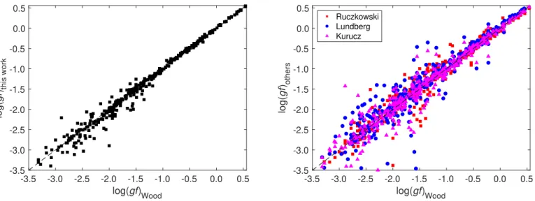
Danzmann & Kock(1980),Kostyk & Orlova(1983),Pickering et al.(2001),Wiese et al.(2001), andMorton(2003) for E1 transi-tions and fromHartman et al.(2005) andDeb et al.(2008) for M1 and E2 transitions. As shown in the figure, the agreement between the log(g f ) values computed in the present work and the respective results from the NIST database are rather good for most of the transitions. Furthermore, the computed log(g f ) values are compared with the results from various exp-erimental sources (Blackwell et al. 1982; Bizzarri et al. 1993;
Pickering et al. 2001,2002;Wood et al. 2013), which were car-ried out by a combination of LIF and FTS methods, as seen in Figs.2–5in the left panels for the present work and the right pan-els for other recent theoretical results (Ruczkowski et al. 2014;
-3.0 -2.5 -2.0 -1.5 -1.0 -0.5 0.0 0.5 log(gf)Pickering -3.0 -2.5 -2.0 -1.5 -1.0 -0.5 0.0 0.5 log( gf )this work -3.0 -2.5 -2.0 -1.5 -1.0 -0.5 0.0 0.5 log(gf)Pickering -3.0 -2.5 -2.0 -1.5 -1.0 -0.5 0.0 0.5 log( gf ) others Ruczkowski Lundberg Kurucz
Fig. 4.Comparison of the theoretical log(g f ) values to those published byPickering et al.(2001,2002). Left panel: this work (black square). Right
panel:Ruczkowski et al.(2014) (red square);Lundberg et al.(2016) (blue circle); andKurucz(2017) (magenta triangle).
-3.5 -3.0 -2.5 -2.0 -1.5 -1.0 -0.5 0.0 0.5 log(gf)Wood -3.5 -3.0 -2.5 -2.0 -1.5 -1.0 -0.5 0.0 0.5 log( gf ) this work -3.5 -3.0 -2.5 -2.0 -1.5 -1.0 -0.5 0.0 0.5 log(gf)Wood -3.5 -3.0 -2.5 -2.0 -1.5 -1.0 -0.5 0.0 0.5 log( gf ) others Ruczkowski Lundberg Kurucz
Fig. 5.Comparison of the theoretical log(g f ) values to those published byWood et al.(2013). Left panel: this work (black square). Right panel:
Ruczkowski et al.(2014) (red square);Lundberg et al.(2016) (blue circle); andKurucz(2017) (magenta triangle).
Table 4. Comparison between experimental and calculated oscillator strengths (log(g f )) for the VUV resonance transitions.
log(g f )
Upper Lower λ(Å) Present HFR(a) Semi-empirical(b) Exp.(c) Exp.(d) Exp.new(d) 3d4s4p4Fo
3/2 3d 24s4F
3/2 1910.612 −0.363 −0.38 −0.372 −0.381(16.7) −0.41(9) 0.388
3d4s4p4Do1/2 3d24s4F3/2 1910.954 −0.398 −0.54 −0.470 −0.407(13.3) −0.55(8) 0.400
References. (a)Lundberg et al.(2016);(b)Kurucz(2017);(c)Wiese et al.(2001); and(d)Pickering et al.(2001).
Lundberg et al. 2016;Kurucz 2017). From the figures, we note an overall better agreement between the present results and experimental values, especially for transitions with log(g f ) ≥ 1.0. The comparisons between other theoretical values, that is, semi-empirical calculations (Ruczkowski et al. 2014; Kurucz 2017) and HFR calculations (Lundberg et al. 2016) as well as experi-mental results show a much wider scatter.
In Table4, the computed and measured log(g f ) values for the two VUV resonance transitions are given. Wiese et al.
(2001) measured the log(g f ) values using the HSAS experiment at the Synchrotron Radiation Center in Stoughton, Wisconsin.
Pickering et al.(2001) determined the two values by a
combi-nation of FTS branching fractions and Kurucz’s calculated life-times. The discrepancy between the values obtained from the two different methods are quite large for the 1910.954 Å tran-sition, and the present computed value is in good agreement with the one from Wiese et al. (2001). We have revised the
Pickering et al. (2001) data by combining their BFs with our lifetimes, which should be more accurate than previous calcula-tions. The new data is included in the last column in Table4. It can be seen that the new log(g f ) values are in excellent agree-ment with those fromWiese et al.(2001).
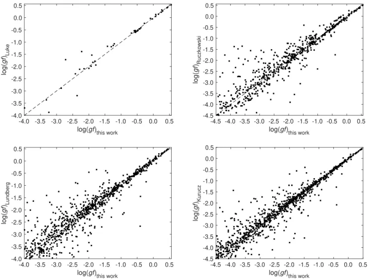
In addition, the present work can be compared with other the-oretical calculations. In Fig.6, log(g f ) values from the present
-4.0 -3.5 -3.0 -2.5 -2.0 -1.5 -1.0 -0.5 0.0 0.5
log(gf)this work
-4.0 -3.5 -3.0 -2.5 -2.0 -1.5 -1.0 -0.5 0.0 0.5 log( gf ) Luke -4.5 -4.0 -3.5 -3.0 -2.5 -2.0 -1.5 -1.0 -0.5 0.0 0.5
log(gf)this work
-4.5 -4.0 -3.5 -3.0 -2.5 -2.0 -1.5 -1.0 -0.5 0.0 0.5 log( gf ) Ruczkowski -4.0 -3.5 -3.0 -2.5 -2.0 -1.5 -1.0 -0.5 0.0 0.5
log(gf)this work
-4.0 -3.5 -3.0 -2.5 -2.0 -1.5 -1.0 -0.5 0.0 0.5 log( gf ) Lundberg -4.5 -4.0 -3.5 -3.0 -2.5 -2.0 -1.5 -1.0 -0.5 0.0 0.5
log(gf)this work
-4.5 -4.0 -3.5 -3.0 -2.5 -2.0 -1.5 -1.0 -0.5 0.0 0.5 log( gf ) Kurucz
Fig. 6.Comparison of log(g f ) values of the current study with the values from other theoretical work. Top left:Luke(1999). Top right:Ruczkowski
et al.(2014). Bottom left:Lundberg et al.(2016). Bottom right:Kurucz(2017).
Table 5. Comparison between experimental and calculated forbidden transition probabilities.
A(s−1)
Upper Lower Type λ(Å) Present CI(a) HFR(B)(b) Semi-empirical(c) Exp.(d)
3d4s2 2D3/2 3d2(3F)4s2F5/2 M1,E2 4918.226 2.314 4.127 3.18 2.338 2.15(20) 3d2(3F)4s2F 7/2 E2 4984.182 0.366 0.662 0.50 0.367 0.42(8) 3d2(1D)4s2D 3/2 M1,E2 6153.610 0.311 0.349 0.34 0.343 0.53(16) 3d2(1D)4s2D5/2 M1,E2 6166.426 0.106 0.106 0.11 0.119 0.048(16) 3d3 2G 7/2 E2 6264.328 0.182 0.143 0.16 0.267 0.20(9) 3d4s2 2D 5/2 3d2(3F)4s2F7/2 M1,E2 4927.262 2.087 3.881 2.90 2.074 1.9(3) 3d2(1D)4s2D5/2 M1,E2 6079.536 0.364 0.410 0.40 0.399 0.41(9) 3d3 2G 9/2 E2 6220.964 0.188 0.146 0.17 0.276 0.19(5)
References. (a)Deb et al.(2008);(b)Palmeri et al.(2008);(c)Kurucz(2017); and(d)Hartman et al.(2005).
work are compared with the results from CI (Luke 1999) as well as semi-empirical (Ruczkowski et al. 2014;Kurucz 2017) and HFR (Lundberg et al. 2016) calculations, when available. As shown in the figure, the deviations between the log(g f ) values computed in the present work and respective results from other sources are small for values down to −1.5, with a much wider scatter for the weaker lines. Given the overall good agreement between the present work and experimental results observed
in the above mentioned discussions, we suggest that the cur-rent results together with the experimental values are used as a reference.
For the M1 and E2 forbidden transitions, there are a num-ber of measurements of transition rates A. In Table 5, the computed A values are compared with experimental results by
Hartman et al.(2005), which were obtained using a combination of laboratory and astrophysical measurements. The computed
-10 -9 -8 -7 -6 -5 -4 -3 -2 -1 0 1
log(A)this work
-3.0 -2.5 -2.0 -1.5 -1.0 -0.5 0.0 0.5 1.0 1.5 2.0 2.5 3.0 log( A ) Deb -log( A ) this work
Fig. 7. Comparison of log(A) values for M1+E2 transitions between
even states of the current study with the values fromDeb et al.(2008).
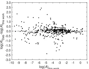
Avalues from the present work and semi-empirical calculations from Kurucz’s database (Kurucz 2017) are in much better agree-ment with those measureagree-ments than from the other theoretical results, that is, the HFR calculation byPalmeri et al.(2008) and the CI calculation byDeb et al.(2008), which were compiled in the NIST ASD. Computed A values from the present work are within the uncertainties of experimental measurements, except for transitions 3d4s2 2D3/2– 3d2(1D)4s2D3/2,5/2, for which, on the contrary, the various theoretical works give much closer val-ues. Finally, in Fig. 7, we compare the computed M1 and E2 transition rates with values from the CI calculations byDeb et al.
(2008). As shown in the figure, the deviations are small for most of the strong transitions, but with a much wider scatter for the weaker lines.
4.3. Lifetimes
The calculated lifetimes are compared with other theoretical pre-dictions and experimental values, when available, in TablesA.2
and A.3 for even and odd states, respectively. The agreement with Kurucz’s semi-empirical results (Kurucz 2017) is overall good for both even and odd states.
In Fig.8, the lifetimes from experiments (Palmeri et al. 2008;
Hartman et al. 2003, 2005) using the LPT approach are com-pared with the results from the present calculations and from other theoretical works (Kurucz 2017;Deb et al. 2008;Palmeri et al. 2008; Grant 1974; Bautista et al. 2006). As can be seen from the figure, the theoretical values from this work fall into, or only slightly outside, the range of the estimated uncertain-ties of the experimental values. On the contrary, the differences between the measured and computed lifetimes by Deb et al.
(2008), using the CIV3 code, are larger for all of these values. For odd states, a number of measurements of lifetimes (Roberts et al. 1973;Kwiatkowski et al. 1985; Gosselin et al. 1987; Bizzarri et al. 1993; Langhans et al. 1995; Lundberg et al. 2016) are compared with the theoretical results from the present work, semi-empirical calculations (Ruczkowski et al. 2016; Kurucz 2017), and HFR calculations (Lundberg et al. 2016). As shown in the figure, the measured lifetimes from
Roberts et al. (1973) are overall larger than the values from other measurements, and all the calculated values from the present work agree with those of the latter within the experi-mental errors. The Kurucz’s values, which are frequently used
20 22 24 26 28 30 32 34 ilev 0.0 5.0 10.0 15.0 20.0 25.0 30.0 35.0 lifetime (s) This work: MCDHF (a): Semi-empirical (b): CI (c): HFR (c): LPT (d): AUTOSTRUCTURE (e): LPT (f): LPT 20 22 12 13 14 15 29 30 6.5 7.0 7.5 8.0 8.5 9.0 33 34 0.18 0.20 0.22 0.24 0.26 0.28 0.30 0.32 0.34 0.36
Fig. 8.Comparison of the experimental (with error bars) and calculated
lifetimes (in s) for even states of Ti
ii
. (a)Kurucz(2017); (b)Deb et al.(2008); (c)Palmeri et al.(2008); (d)Bautista et al.(2006); (e)Hartman
et al.(2005); and (f)Hartman et al.(2003). We note that ilev, a label in
the x-axis, corresponds to the ilev in TableA.1.
as a reference in many literature, are in agreement with experi-mental values in most cases, except for the 3d2(3
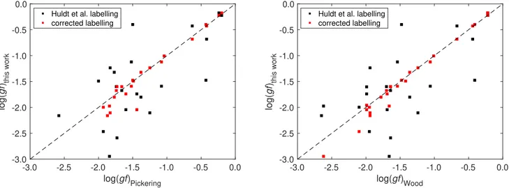
2F) 3F4p2Go 7/2, 3d2(12D)1D4p2Do 5/2, and 3d 2(1 2D) 1D4p2Fo 5/2levels. 4.4. Labelling of the 3d2(1 2D)4p y 2Do 3/2and z 2Po 3/2levels The NIST label classification for Ti
ii
adheres to the analysis byHuldt et al. (1982), who assigned the 39 603 cm−1 level as 3d2(1 2D)4p 2Do 3/2 and the 39 233 cm −1 level as 2Po 3/2. Due to the strong mixing between the states, the assignment is uncer-tain and it was later questioned byBizzarri et al.(1993). Based on lifetime measurements, they suggested that the assignments for the two levels should be interchanged. However, they did not update the identifications, according to their suggestion, and the lifetime values and oscillator strengths in later pub-lications (Pickering et al. 2001, 2002; Wood et al. 2013) are presented using the original identification. The present calcu-lations support the suggestion of Bizzarri. Our calculated level energies are 39 357 cm−1 for 2Do3/2 and 39 723 cm
−1 for 2Po 3/2, suggesting the experimental level 39 233 cm−1 to be2Do
3/2 and the level 39 603 cm−1to be2Po3/2. By reassigning the two levels, there is also a significant improvement in the agreement between our theoretical and the measured log(g f ) values. As shown in Fig.10, after correcting the labels, the agreement is very good for most of the transitions. Further support for the reassignment is offered by the lifetimes, which are 5.48 and 4.42 ns, respectively, for2Do
3/2and 2Po
3/2from the present work, relative to 4.5(2) and 5.5(3) ns fromBizzarri et al.(1993) using the original identifica-tions. Again, the reassignment of the two levels results in a per-fect agreement between the theoretical and measured lifetimes (see TableA.3). Please note that all the labels in this paper have been corrected to the new labels.
5. Summary and conclusions
In the present work, extended transition data of E1, M1, and E2 transitions and lifetimes are made available for Ti
ii
using MCDHF and RCI methods. The computations of transition prop-erties in the systems of Tiii
are challenging, mainly due to the strong interaction between the terms and configurations of35 40 45 50 55 60 65 70 75 80 85 90 95 100 ilev 2.0 2.5 3.0 3.5 4.0 4.5 5.0 5.5 6.0 6.5 7.0 7.5 8.0 8.5 lifetime (ns) This work: MCDHF (a): Semi-empirical (b): Semi-empirical (c): LIF (d): LIF (e): Beam-foil (f): LIF (g): Beam-laser (h): HFR (h): LIF
Fig. 9.Comparison of the experimental (with error bars) and calculated lifetimes (in ns) for odd states of Ti
ii
. (a)Kurucz(2017); (b)Ruczkowskiet al.(2016); (c)Bizzarri et al.(1993); (d)Kwiatkowski et al.(1985); (e)Roberts et al.(1973); (f)Langhans et al.(1995); (g)Gosselin et al.
(1987); and (h)Lundberg et al.(2016). We note that ilev, a label in the x-axis, corresponds to the ilev in TableA.1.
-3.0 -2.5 -2.0 -1.5 -1.0 -0.5 0.0 log(gf)Pickering -3.0 -2.5 -2.0 -1.5 -1.0 -0.5 0.0 log( gf ) this work
Huldt et al. labelling corrected labelling -3.0 -2.5 -2.0 -1.5 -1.0 -0.5 0.0 log(gf)Wood -3.0 -2.5 -2.0 -1.5 -1.0 -0.5 0.0 log( gf ) this work
Huldt et al. labelling corrected labelling
Fig. 10.Comparison of the theoretical log(g f ) values for the transitions involving 3d2(1
2D)4p 2D
3/2or2P3/2levels to measured values byPickering
et al.(2001,2002) andWood et al.(2013), both before and after the interchange of the labelling of the two levels.
the even states. Thus, some of the states are strongly mixed, and highly correlated wave functions are needed to accurately predict their LS -composition. It is found that the inclusion of {3p43d44s, 3p43d34s2 and 3p43d5} configurations in MR is very important to predict the correct order of the even energy levels.
We have performed an extensive comparison of the com-puted oscillator strengths and lifetimes with other theoretical and experimental results. There is a significant improvement in the accuracy in the computed oscillator strengths of E1 transitions compared with previous theoretical works.
The computed lifetimes of odd states are all in excellent agreement with the measured lifetimes. We suggest that the cur-rent results be used as a reference for Ti
ii
for various astrophys-ical applications.A careful comparison of the energies of the levels, the oscil-lator strengths, as well as the radiative lifetimes with the experimental values has made possible the identification of the mislabelling of the 3d2(1 2D)4p y 2Do 3/2and z 2Po 3/2levels adopted in the NIST ASD. The assignments for the2Do
3/2and 2Po
3/2levels should be interchanged.
Acknowledgements. This work is supported by the Swedish research coun-cil under contracts 2015-04842 and 2016-04185. Kai Wang acknowledges the support from the National Natural Science Foundation of China (Grant No. 11703004), the Natural Science Foundation of Hebei Province, China (A2019201300), and the Natural Science Foundation of Educational Depart-ment of Hebei Province, China (BJ2018058). We would also like to thank the anonymous referee for her/his useful comments that helped improve the original manuscript.
References
Abrahamsson, K., Andler, G., Bagge, L., et al. 1993,Nucl. Instrum. Methods
Phys. Res. Sect. B: Beam Interact. Mater. At., 79, 269
Aldenius, M. 2009,Phys. Scr., T134, 014008
Allende Prieto, C., & Garcia Lopez, R. J. 1998,A&AS, 131, 431
Badnell, N. R. 1986,J. Phys. B: At. Mol. Phys., 19, 3827
Bautista, M. A., Hartman, H., Gull, T. R., Smith, N., & Lodders, K. 2006,
MNRAS, 370, 1991
Bizzarri, A., Huber, M. C. E., Noels, A., et al. 1993,A&A, 273, 707
Blackwell, D. E., Menon, S. L. R., & Petford, A. D. 1982,MNRAS, 201, 603
Cowan, R. D. 1981,The Theory of Atomic Structure and Spectra((Berkeley,
CA: University of California Press))
Cowan, J. J., Sneden, C., Roederer, I. U., et al. 2020,ApJ, 890, 119
Danzmann, K., & Kock, M. 1980,J. Phys. B: At. Mol. Phys., 13, 2051
Deb, N. C., Hibbert, A., Felfli, Z., & Msezane, A. Z. 2008,J. Phys. B: At. Mol. Opt. Phys., 42, 015701
Dyall, K., Grant, I., Johnson, C., Parpia, F., & Plummer, E. 1989,Comput. Phys. Commun., 55, 425
Ekman, J., Godefroid, M., & Hartman, H. 2014,Atoms, 2, 215
Froese Fischer, C. 2009,Phys. Scr. Vol. T, 134, 014019
Froese Fischer, C., Godefroid, M., Brage, T., Jönsson, P., & Gaigalas, G. 2016,
J. Phys. B: At. Mol. Opt. Phys, 49, 182004
Froese Fischer, C., Gaigalas, G., Jönsson, P., & Biero´n, J. 2019,Comput. Phys. Commun., 237, 184
Gaigalas, G., Rudzikas, Z., & Froese Fischer, C. 1997,J. Phys. B At. Mol. Phys., 30, 3747
Gaigalas, G., Fritzsche, S., & Grant, I. P. 2001,Comput. Phys. Commun., 139, 263
Gaigalas, G., Froese Fischer, C., Rynkun, P., & Jönsson, P. 2017,Atoms, 5, 6
Gosselin, R., Pinnington, E., & Ansbacher, W. 1987,Phys. Lett. A, 123, 175
Grant, I. P. 1974,J. Phys. B: At. Mol. Opt. Phys, 7, 1458
Grant, I. P. 2007, Relativistic Quantum Theory of Atoms and Molecules
(New York: Springer)
Hartman, H., Rostohar, D., Derkatch, A., et al. 2003,J. Phys. B: At. Mol. Opt. Phys., 36, L197
Hartman, H., Gull, T., Johansson, S., Smith, N., & Team, H. E. C. T. P. 2004,
A&A, 419, 215
Hartman, H., Schef, P., Lundin, P., et al. 2005,MNRAS, 361, 206
Hibbert, A. 1974,J. Phys. B: At. Mol. Phys., 7, 1417
Hibbert, A. 1975,Comput. Phys. Commun., 9, 141
Huldt, S., Johansson, S., Litzén, U., & Wyart, J.-F. 1982,Phys. Scr., 25, 401
Kostyk, R. I., & Orlova, T. V. 1983,Astrometriia i Astrofizika, 49, 39
Kramida, A., Ralchenko, Y., Reader, J., & NIST ASD Team 2019, NIST
Atomic Spectra Database (ver. 5.7.1)(Gaithersburg, MD: National Institute
of Standards and Technology),https://physics.nist.gov/asd[2020,
May 13]
Kurucz, R. L. 2017, On-line Database of Observed and Predicted Atomic
Transitions(Cambridge, MA: Harvard-Smithsonian Center for Astrophysics),
http://kurucz.harvard.edu
Kwiatkowski, M., Werner, K., & Zimmermann, P. 1985, Phys. Rev. A, 31,
2695
Langhans, G., Schade, W., & Helbig, V. 1995,Z. Phys. D At. Mol. Clusters, 34, 151
Li, W., Rynkun, P., Radži¯ut˙e, L., et al. 2020,A&A, 639, A25
Lidberg, J., Al-Khalili, A., Norlin, L. O., et al. 1999,Nucl. Instrum. Methods Phys. Res. Sect. B: Beam Interact. Mater. At., 152, 157
Luke, T. M. 1999,Can. J. Phys., 77, 571
Lundberg, H., Hartman, H., Engström, L., et al. 2016,MNRAS, 460, 356
McKenzie, B. J., Grant, I. P., & Norrington, P. H. 1980,Comput. Phys. Commun., 21, 233
Morton, D. C. 2003,ApJS, 149, 205
Morton, D. C. 2004,ApJS, 151, 403
Olsen, J., Roos, B. O., Jørgensen, P., & Jensen, H. J. A. 1988,J. Chem. Phys., 89, 2185
Palmeri, P., Quinet, P., Biémont, É., et al. 2008,J. Phys. B: At. Mol. Opt. Phys., 41, 125703
Pickering, J. C., Thorne, A. P., & Perez, R. 2001,ApJS, 132, 403
Pickering, J. C., Thorne, A. P., & Perez, R. 2002,ApJS, 138, 247
Roberts, J. R., Andersen, T., & Sorensen, G. 1973,ApJ, 181, 567
Roberts, J. R., Voigt, P. A., & Czernichowski, A. 1975,ApJ, 197, 791
Ruczkowski, J., Elantkowska, M., & Dembczynski, J. 2014,J. Quant. Spectrosc. Radiat. Transfer, 149, 168
Ruczkowski, J., Elantkowska, M., & Dembczynski, J. 2016,J. Quant. Spectrosc. Radiat. Transfer, 176, 6
Ryde, N. 2009,Physica Scripta, T134, 014001
Saloman, E. B. 2012,J. Phys. Chem. Ref. Data, 41, 013101
Savanov, I. S., Huovelin, J., & Tuominen, I. 1990,A&AS, 86, 531
Sneden, C., Cowan, J. J., Kobayashi, C., et al. 2016,ApJ, 817, 53
Sturesson, L., Jönsson, P., & Froese Fischer, C. 2007,CoPhC, 177, 539
Sugar, J., & Corliss, C. 1985,J. Phys. Chem. Ref. Data, 14, 2
Thevenin, F. 1989,A&AS, 77, 137
Wiese, L. M., Fedchak, J. A., & Lawler, J. E. 2001,ApJ, 547, 1178
Wolnik, S. J., & Berthel, R. O. 1973,ApJ, 179, 665
Wood, M. P., Lawler, J. E., Sneden, C., & Cowan, J. J. 2013, ApJS, 208,
Appendix A: Atomic state function composition in LS-coupling, energy levels, and lifetimes for the Ti ii ion.
Table A.1. Atomic state function composition (up to three LS components with a contribution>0.02 of the total wave function) in LS -coupling and energy levels (in cm−1) for Ti II.
ilev State LS-composition ERCI ENIS T
1 3d2(32F)3F4s4F3/2 0.93 0 0 2 3d2(32F)3F4s4F5/2 0.93 90 94 3 3d2(32F)3F4s4F7/2 0.93 215 226 4 3d2(3 2F) 3F4s4F 9/2 0.93 375 393 5 3d3(4 3F) 4F 3/2 0.94 963 908 6 3d3(4 3F) 4F 5/2 0.94 1 034 984 7 3d3(4 3F) 4F 7/2 0.94 1 132 1 087 8 3d3(4 3F) 4F 9/2 0.94 1 253 1 216 9 3d2(3 2F) 3F4s2F 5/2 0.90 4 775 4 629 10 3d2(3 2F) 3F4s2F 7/2 0.90 5 032 4 898 11 3d2(1 2D)1D4s2D3/2 0.71+ 0.14 3p63d3(32D)2D+ 0.05 3p63d3(21D)2D 8 835 8 711 12 3d2(1 2D)1D4s2D5/2 0.73+ 0.13 3p63d3(32D)2D+ 0.05 3p63d3(21D)2D 8 867 8 744 13 3d3(2 3G)2G7/2 0.89+ 0.04 3p63d2(12G)1G4s2G 9 256 8 998 14 3d3(2 3G)2G9/2 0.89+ 0.04 3p63d2(12G)1G4s2G 9 370 9 118 15 3d3(4 3P)4P1/2 0.85+ 0.04 3p63d2(32P)3P4s4P+ 0.03 3p63d3(23P)2P 9 506 9 364 16 3d3(43P)4P3/2 0.82+ 0.05 3p63d3(23P) 2P+ 0.04 3p63d2(3 2P) 3P4s4P 9 537 9 396 17 3d3(43P)4P5/2 0.89+ 0.04 3p63d2(32P) 3P4s4P 9 655 9 518 18 3d3(23P)2P1/2 0.61+ 0.26 3p63d2(32P) 3P4s2P+ 0.03 3p63d2(3 2P) 3P4s4P 9 938 9 851 19 3d2(32P)3P4s4P1/2 0.86+ 0.06 3p63d3(43P)4P 9 969 9 873 20 3d2(32P)3P4s4P3/2 0.89+ 0.04 3p63d3(43P)4P 10 022 9 931 21 3d3(23P)2P3/2 0.59+ 0.25 3p63d2(32P)3P4s2P+ 0.07 3p63d3(43P)4P 10 057 9 976 22 3d2(3 2P) 3P4s4P 5/2 0.88+ 0.04 3p63d3(43P)4P 10 111 10 025 23 3d3(2 3D) 2D 3/2 0.51+ 0.20 3p63d3(21D)2D+ 0.20 3p63d2(12D)1D4s2D 12 920 12 629 24 3d3(2 3D) 2D 5/2 0.52+ 0.20 3p63d3(21D)2D+ 0.19 3p63d2(12D)1D4s2D 13 043 12 758 25 3d3(2 3H) 2H 9/2 0.93 13 061 12 677 26 3d3(2 3H) 2H 11/2 0.93 13 154 12 775 27 3d2(1 2G) 1G4s2G 9/2 0.89+ 0.04 3p63d3(23G)2G 15 598 15 258 28 3d2(1 2G)1G4s2G7/2 0.89+ 0.04 3p63d3(23G)2G 15 607 15 266 29 3d2(3 2P) 3P4s2P 1/2 0.64+ 0.27 3p63d3(23P)2P 16 889 16 516 30 3d2(3 2P) 3P4s2P 3/2 0.64+ 0.27 3p63d3(23P)2P 16 992 16 625 31 3d3(2 3F)2F7/2 0.91 21 358 20 892 32 3d3(2 3F)2F5/2 0.91 21 415 20 952 33 3d2D4s2 2D 3/2 0.64+ 0.12 3p63d3(23D)2D+ 0.11 3p63d3(21D)2D 25 080 24 961 34 3d2D4s2 2D5/2 0.62+ 0.12 3p63d3(21D) 2D+ 0.12 3p63d3(2 3D) 2D 25 316 25 193 35 3d2(32F)3F4p4G◦5/2 0.93 29 561 29 544 36 3d2(3 2F) 3F4p4G◦ 7/2 0.94 29 744 29 735 37 3d2(3 2F) 3F4p4G◦ 9/2 0.94 29 969 29 968 38 3d2(32F)3F4p4G◦11/2 0.94 30 233 30 241 39 3d2(3 2F)3F4p4F ◦ 3/2 0.92+ 0.02 3p63d2(32F)3F4p2D ◦ 30 818 30 836 40 3d2(3 2F) 3F4p4F◦ 5/2 0.93 30 935 30 959 41 3d2(32F)3F4p4F◦7/2 0.93 31 084 31 114 42 3d2(3 2F)3F4p2F ◦ 5/2 0.78+ 0.08 3p63d2(12D)1D4p2F ◦+ 0.03 3p63d2(3 2F)3F4p2D ◦ 31 258 31 208 43 3d2(3 2F) 3F4p4F◦ 9/2 0.94 31 263 31 301 44 3d2(32F)3F4p2F◦7/2 0.82+ 0.08 3p63d2(12D)1D4p2F◦ 31 530 31 491 45 3d2(3 2F)3F4p2D ◦ 3/2 0.77+ 0.08 3p63d2(32P)3P4p2D ◦ + 0.02 3p63d2(3 2F)3F4p4D ◦ 31 779 31 757 46 3d2(3 2F) 3F4p2D◦ 5/2 0.72+ 0.08 3p 63d2(3 2P) 3P4p2D◦+ 0.05 3p63d2(3 2F) 3F4p4D◦ 32 038 32 026 47 3d2(10S)1S4s2S1/2 0.92 32 129 31 788 48 3d2(3 2F) 3F4p4D◦ 1/2 0.92 32 527 32 532 49 3d2(32F)3F4p4D◦3/2 0.89+ 0.02 3p63d2(32F)3F4p2D◦ 32 593 32 603 50 3d2(3 2F) 3F4p4D◦ 5/2 0.86+ 0.05 3p 63d2(3 2F) 3F4p2D◦ 32 683 32 698 51 3d2(3 2F) 3F4p4D◦ 7/2 0.91 32 746 32 767 52 3d3(21D)2D3/2 0.52+ 0.19 3p63d2D4s2 2D+ 0.15 3p63d3(23D) 2D 32 754 32 275 53 3d3(21D)2D5/2 0.52+ 0.20 3p63d2D4s2 2D+ 0.14 3p63d3(23D) 2D 32 798 32 333
Table A.1. continued.
ilev State LS-composition ERCI ENIS T
54 3d2(32F)3F4p2G◦7/2 0.89+ 0.05 3p63d2(12G)1G4p2G◦ 34 742 34 543 55 3d2(3 2F) 3F4p2G◦ 9/2 0.89+ 0.05 3p63d2(12G)1G4p2G ◦ 34 936 34 749 56 3d2(3 2P) 3P4p2S◦ 1/2 0.94 37 499 37 431 57 3d2(12D)1D4p2D◦3/2 0.51+ 0.29 3p63d2(12D)1D4p2P◦+ 0.05 3p63d2(32P)3P4p2D◦ 39 357 39 233 58 3d2(1 2D)1D4p2D ◦ 5/2 0.70+ 0.06 3p63d2(32P)3P4p2D ◦+ 0.05 3p63d2D4s3D4p2D◦ 39 599 39 477 59 3d2(1 2D) 1D4p2P◦ 3/2 0.58+ 0.24 3p 63d2(1 2D) 1D4p2D◦+ 0.05 3p63d2(3 2P) 3P4p4S◦ 39 723 39 603 60 3d2(12D)1D4p2P◦1/2 0.92 39 789 39 675 61 3d2(1 2D)1D4p2F ◦ 5/2 0.77+ 0.09 3p63d2(32F)3F4p2F ◦ + 0.05 3p63d2(1 2D)1D4p2D ◦ 40 143 39 927 62 3d2(3 2P) 3P4p4S◦ 3/2 0.89+ 0.05 3p 63d2(1 2D) 1D4p2P◦ 40 200 40 027 63 3d2(12D)1D4p2F◦7/2 0.77+ 0.09 3p63d2(32F)3F4p2F◦+ 0.06 3p63d2(32P)3P4p4D◦ 40 292 40 075 64 3d2(3 2P)3P4p4D ◦ 1/2 0.92 40 423 40 330 65 3d2(3 2P) 3P4p4D◦ 3/2 0.91 40 515 40 426 66 3d2(3 2P) 3P4p4D◦ 5/2 0.90 40 668 40 582 67 3d2(32P)3P4p4D◦7/2 0.86+ 0.05 3p63d2(12D)1D4p2F◦ 40 883 40 798 68 3d2(3 2P) 3P4p4P◦ 1/2 0.91+ 0.03 3p63d2D4s3D4p4P ◦ 42 084 41 997 69 3d2(3 2P) 3P4p4P◦ 3/2 0.91+ 0.03 3p 63d2D4s3D4p4P◦ 42 154 42 069 70 3d2(32P)3P4p4P◦5/2 0.90+ 0.03 3p63d2D4s3D4p4P◦ 42 289 42 209 71 3d2(1 2G)1G4p2G ◦ 7/2 0.89+ 0.05 3p63d2(32F)3F4p2G ◦ 44 088 43 741 72 3d2(1 2G) 1G4p2G◦ 9/2 0.88+ 0.05 3p 63d2(3 2F) 3F4p2G◦ 44 127 43 781 73 3d2(32P)3P4p2D◦5/2 0.76+ 0.09 3p63d2(12D)1D4p2D◦+ 0.05 3p63d2(32F)3F4p2D◦ 45 286 44 902 74 3d2(3 2P)3P4p2D ◦ 3/2 0.74+ 0.09 3p63d2(12D)1D4p2D ◦+ 0.04 3p63d2(3 2F)3F4p2D ◦ 45 296 44 915 75 3d2(3 2P) 3P4p2P◦ 1/2 0.87+ 0.03 3p 63d2D4s3D4p2P◦+ 0.02 3p63d2D4s1D4p2P◦ 45 761 45 472 76 3d2(32P)3P4p2P◦3/2 0.84+ 0.03 3p63d2D4s3D4p2P◦+ 0.02 3p63d2(23P)3P4p2D◦ 45 839 45 549 77 3d2(1 2G)1G4p2H ◦ 9/2 0.93 46 047 45 674 78 3d2(1 2G) 1G4p2H◦ 11/2 0.94 46 277 45 909 79 3d2(1 2G) 1G4p2F◦ 7/2 0.84+ 0.07 3p 63d2D4s3D4p2F◦+ 0.02 3p63d2(1 2D) 1D4p2F◦ 47 737 47 467 80 3d2(12G)1G4p2F5/2◦ 0.84+ 0.07 3p63d2D4s3D4p2F◦+ 0.02 3p63d2(12D)1D4p2F◦ 47 893 47 625 81 3d2D4s3D4p4F◦ 3/2 0.73+ 0.15 3p 63d2D4s3D4p4D◦ 52 134 52 330 82 3d2D4s3D4p4D◦ 1/2 0.88 52 184 52 339 83 3d2D4s3D4p4F5/2◦ 0.61+ 0.27 3p63d2D4s3D4p4D◦ 52 280 52 472 84 3d2D4s3D4p4D◦ 3/2 0.73+ 0.16 3p63d2D4s3D4p4F ◦ 52 288 52 459 85 3d2D4s3D4p4D◦ 5/2 0.60+ 0.29 3p 63d2D4s3D4p4F◦ 52 447 52 631 86 3d2D4s3D4p4F7/2◦ 0.51+ 0.39 3p63d2D4s3D4p4D◦+ 0.02 3p63d2D4s3D5p2F◦ 52 510 52 705 87 3d2D4s3D4p4D◦ 7/2 0.49+ 0.40 3p63d2D4s3D4p4F ◦ 52 650 52 847 88 3d2D4s3D4p4F◦ 9/2 0.90+ 0.02 3p 63d2D4s3D5p4F◦ 52 866 53 097 89 3d2D4s1D4p2D◦5/2 0.53+ 0.28 3p63d2D4s3D4p2D◦+ 0.06 3p63d2(21D)1D4p2D◦ 53 507 53 555 90 3d2D4s1D4p2D◦ 3/2 0.53+ 0.28 3p63d2D4s3D4p2D ◦+ 0.06 3p63d2(1 2D)1D4p2D ◦ 53 546 53 597 91 3d2D4s3D4p4P◦ 1/2 0.89+ 0.03 3p 63d2(3 2P) 3P4p4P◦ 56 030 56 223 92 3d2D4s3D4p4P◦3/2 0.88+ 0.03 3p63d2(32P)3P4p4P◦ 56 054 56 249 93 3d2D4s3D4p4P◦ 5/2 0.88+ 0.03 3p63d2(32P)3P4p4P ◦ 56 124 56 326 94 3d2D4s1D4p2F◦ 5/2 0.73+ 0.14 3p 63d2D4s3D4p2F◦+ 0.04 3p63d2(1 2G) 1G4p2F◦ 59 328 59 322 95 3d2D4s1D4p2P3/2◦ 0.46+ 0.27 3p63d2D4s3D4p2P◦+ 0.17 3p63d2(10S)1S4p2P◦ 59 411 59 388 96 3d2D4s1D4p2F◦ 7/2 0.72+ 0.15 3p63d2D4s3D4p2F ◦ + 0.04 3p63d2(1 2G)1G4p2F ◦ 59 476 59 468 97 3d2D4s1D4p2P◦ 1/2 0.42+ 0.27 3p 63d2D4s3D4p2P◦+ 0.21 3p63d2(1 0S) 1S4p2P◦ 59 485 59 440 98 3d2(1 0S) 1S4p2P◦ 1/2 0.62+ 0.25 3p 63d2D4s1D4p2P◦+ 0.03 3p63d2(3 2P) 3P4p2P◦ 63 812 63 277 99 3d2(10S)1S4p2P◦3/2 0.65+ 0.22 3p63d2D4s1D4p2P◦+ 0.03 3p63d2(32P)3P4p2P◦ 63 930 63 375
Table A.2. Comparison of the experimental (with the uncertainty in the last digit given in parentheses) and calculated lifetimes (in s) for even states of Ti II.
State This work Other calculations Experiments
3d2(3 2F)4s
4F
5/2 3.192e+4 2.770e+4(a); 2.77e+4(b)
3d2(3
2F)4s4F7/2 1.167e+4 1.008e+4(a); 1.01e+4(b)
3d2(3 2F)4s
4F
9/2 9.070e+3 7.813e+3(a); 7.83e+3(b)
3d3(4
3F)4F3/2 9.994e+5 1.189e+6(a); 1.47e+6(b)
3d3(4
3F)4F5/2 5.940e+4 5.025e+4(a); 5.08e+4(b)
3d3(4
3F)4F7/2 2.428e+4 2.033e+4(a); 2.04e+4(b)
3d3(4
3F)4F9/2 2.041e+4 1.712e+4(a); 1.72e+4(b)
3d2(3
2F)4s2F5/2 4.533e+2 5.000e+2(a); 3.20e+2(b)
3d2(3
2F)4s2F7/2 4.336e+2 4.525e+2(a); 3.19e+2(b)
3d2(1 2D)4s
2D
3/2 8.452e+1 8.130e+1(a); 6.01e+1(b)
3d2(1
2D)4s2D5/2 9.988e+1 9.804e+1(a); 7.08e+1(b)
3d3(2 3G)
2G
7/2 1.694e+2 1.647e+2(a); 1.44e+2(b)
3d3(2
3G)2G9/2 1.166e+2 1.103e+2(a); 9.30e+1(b)
3d3(4 3P)
4P
1/2 1.072e+1 9.434e+0(a); 1.26e+1(b)
3d3(4
3P)4P3/2 1.144e+1 1.010e+1(a); 1.34e+1(b)
3d3(4
3P)4P5/2 1.096e+1 9.709e+0(a); 1.30e+1(b)
3d3(2
3P)2P1/2 1.604e+2 8.197e+1(a); 2.02e+2(b)
3d3(2
3P)2P3/2 9.192e+1 7.299e+1(a); 1.05e+2(b)
3d2(3 2P)4s
4P
1/2 1.297e+1 1.248e+1(a); 1.23e+1(b); 1.36e+1(c); 1.30e+1(d); 1.27e+1(e)
3d2(3
2P)4s4P3/2 1.332e+1 1.222e+1(a); 1.26e+1(b); 2.28e+1(c); 1.43e+1(d); 1.31e+1(e); 3.11e+1( f ) 1.8(4)e+1(g)
3d2(3 2P)4s
4P
5/2 1.379e+1 1.245e+1(a); 1.31e+1(b); 1.43e+1(c); 1.36e+1(d); 1.35e+1(e); 1.64e+1( f ) 2.8(10)e+1(h); 1.6(2)e+1(i)
3d3(2
3D)2D3/2 2.312e+1 2.193e+1(a); 2.73e+1(b); 1.82e+1(c); 1.90e+1(d); 1.81e+1(e)
3d3(2 3D)
2D
5/2 2.767e+1 2.564e+1(a); 3.37e+1(b); 2.15e+1(c); 2.25e+1(d); 2.15e+1(e) 2.4(3)e+1(i)
3d3(2
3H)2H9/2 2.359e+1 2.494e+1(a); 3.33e+1(b)
3d3(2
3H)2H11/2 2.689e+1 2.849e+1(a); 3.97e+1(b)
3d2(1
2G)4s2G9/2 6.523e+1 6.803e+1(a); 5.13e+1(b); 5.62e+1(c); 5.68e+1(d); 5.21e+1(e)
3d2(1
2G)4s2G7/2 7.080e+1 7.299e+1(a); 5.69e+1(b); 5.97e+1(c); 6.05e+1(d); 5.71e+1(e)
3d2(3 2P)4s
2P
1/2 8.243e+0 8.333e+0(a); 8.72e+0(b); 7.21e+0(c); 7.08e+0(d); 7.00e+0(e); 12.7e+0( f ) 14(3)e+0(g); 7.7(7)e+0(i)
3d2(3
2P)4s2P3/2 8.082e+0 8.197e+0(a); 8.48e+0(b); 7.12e+0(c); 7.01e+0(d); 6.87e+0(e) 7.0(6)e+0(i)
3d3(2 3F)
2F
7/2 2.222e+0 2.188e+0(a); 2.97e+0(b); 2.04e+0(c); 2.14e+0(d); 2.34e+0(e)
3d3(2
3F)2F5/2 2.184e+0 2.137e+0(a); 2.95e+0(b); 2.00e+0(c); 2.11e+0(d); 2.31e+0(e)
3d2D4s2 2D
3/2 3.006e−1 2.865e−1(a); 1.8e−1(b); 2.18e−1(c); 2.29e−1(d); 2.17e−1(e); 1.92e−1( f ) 2.9(1)e−1(g)
3d2D4s2 2D
5/2 3.179e−1 3.049e−1(a); 1.9e−1(b); 2.28e−1(c); 2.42e−1(d); 2.29e−1(e); 1.96e−1( f ) 3.3(2)e−1(g)
3d2(1 0S)4s
2S
1/2 2.366e−1 2.096e−1(a)
3d3(2
1D)2D3/2 1.074e−2 2.242e−2(a)
3d3(2
1D)2D5/2 1.532e−2 2.740e−2(a)
References. Semi-empirical:(a)Kurucz(2017); CI:(b)Deb et al.(2008); HFR(A):(c)Palmeri et al.(2008); HFR(B):(d)Palmeri et al.(2008); HFR(C):
(e)Palmeri et al.(2008); AUTOSTRUCTURE:( f )Bautista et al.(2006); LPT:(g)Hartman et al.(2005); LPT:(h)Hartman et al.(2003); and LPT:
(i)Palmeri et al.(2008).
Table A.3. Comparison of the experimental (with the uncertainty in the last digit given in parentheses) and calculated lifetimes (in ns) for odd states of Ti II.
State This work Other calculations Experiments
3d2(3 2F)4p 4Go 5/2 5.659 5.988 (a); 6.1(b) 5.7(3)(c); 5.9(6)(d); 6.6(7)(e) 3d2(3 2F)4p 4Go 7/2 5.598 5.917 (a); 6.0(b) 5.6(3)(c); 5.8(5)(d); 7.8(8)(e) 3d2(3 2F)4p 4Go 9/2 5.520 5.848 (a); 6.0(b) 5.6(3)(c); 5.7(6)(d); 7.3(7)(e) 3d2(3 2F)4p 4Go 11/2 5.434 5.780 (a); 5.9(b) 5.6(3)(c); 5.7(7)(d); 7.2(7)(e) 3d2(3 2F)4p 4Fo 3/2 4.098 4.202 (a); 3.9(b) 4.1(2)(c); 4.2(4)(d); 4.5(3)( f ) 3d2(3 2F)4p 4Fo 5/2 4.057 4.149 (a); 3.8(b); 3.76(g) 4.1(2)(c); 4.1(3)(d); 4.3(3)( f );3.87(20)(h) 3d2(3 2F)4p 4Fo 7/2 4.033 4.132 (a); 3.8(b) 4.1(2)(c); 4.4(6)(d); 4.5(2)( f ) 3d2(3 2F)4p 4Fo 9/2 4.015 4.098 (a); 3.8(b) 4.1(2)(c); 4.3(4)(d); 5.4(8)(e); 4.2(2)( f ) 3d2(3 2F)4p 2Fo 5/2 7.028 7.092 (a); 7.2(b) 6.8(3)(c) 3d2(3 2F)4p 2Fo 7/2 6.896 6.993 (a); 7.1(b) 6.8(3)(c) 3d2(3 2F)4p 2Do 3/2 6.874 6.849 (a); 6.8(b); 5.87(g) 6.6(3)(c); 6.3(10)(d); 6.10(20)(h) 3d2(3 2F)4p 2Do 5/2 6.782 6.757 (a); 6.6(b) 6.6(3)(c); 6.5(9)(d) 3d2(3 2F)4p 4Do 1/2 3.783 3.788 (a); 3.5(b) 3.9(2)(c); 4.0(4)(d); 4.0(3)( f ) 3d2(3 2F)4p 4Do 3/2 3.842 3.846 (a); 3.6(b) 4.0(2)(c); 4.1(5)(d); 4.0(3)( f ) 3d2(3 2F)4p 4Do 5/2 3.911 3.922
(a); 3.7(b); 3.47(g) 4.0(2)(c); 3.9(4)(d); 4.01(6)(i); 5.2(8)(e); 4.2(3)( f ); 3.86(20)(h) 3d2(3
2F)4p 4Do
7/2 3.846 3.846
(a); 3.6(b); 3.40(g) 4.0(2)(c); 4.1(5)(d); 4.2(3)( f ); 3.75(20)(h)
References. Semi-empirical:(a)Kurucz(2017); Semi-empirical:(b)Ruczkowski et al.(2016); LIF:(c)Bizzarri et al.(1993); LIF:(d)Kwiatkowski
et al.(1985); Beam-foil:(e)Roberts et al.(1973); LIF:( f )Langhans et al.(1995); HFR:(g)Lundberg et al.(2016); LIF:(h)Lundberg et al.(2016); and
Table A.3. continued.
State This work Other calculations Experiments
3d2(3 2F)4p 2Go 7/2 4.633 4.854 (a); 5.5(b) 4.6(2)(c); 6.7(16.7)(e) 3d2(3 2F)4p 2Go 9/2 4.642 4.854 (a); 5.5(b) 4.6(2)(c); 4.8(4)(d); 6.2(15.5)(e) 3d2(32P)4p2S1/2o 5.901 5.917(a); 5.0(b) 10.0(>25)(e) 3d2(1 2D)4p 2Do 3/2 5.484 5.495 (a); 5.1(b) 5.5(3)(c); 6.7(>16.7)(e) 3d2(1 2D)4p 2Do 5/2 6.385 5.435 (a); 6.1(b) 6.1(3)(c); 8.0(12)(e) 3d2(1 2D)4p 2Po 3/2 4.422 4.464 (a); 4.2(b) 4.5(2)(c) 3d2(12D)4p2Po1/2 3.864 3.831(a); 3.6(b) 4.0(2)(c) 3d2(1 2D)4p 2Fo 5/2 3.729 4.425 (a); 3.7(b) 3.9(2)(c); 5.9(8.8)(e) 3d2(1 2D)4p 2Fo 7/2 3.644 3.759 (a); 3.5(b) 3.8(2)(c); 4.1(4)(d); 6.7(1)(e) 3d2(3 2P)4p 4So 3/2 3.483 3.521 (a); 3.1(b) 3.6(2)(c); 5.5(8)(e) 3d2(32P)4p4D1/2o 4.311 4.484(a); 3.3(b) 4.4(2)(c); 4.6(5)(d) 3d2(3 2P)4p 4Do 3/2 4.302 4.464 (a); 3.3(b) 4.5(2)(c) 3d2(3 2P)4p 4Do 5/2 4.260 4.425 (a); 3.3(b) 4.3(2)(c); 4.2(6)(d); 6.1(9.1)(e) 3d2(3 2P)4p 4Do 7/2 4.199 4.310 (a); 3.3(b) 4.2(2)(c) 3d2(32P)4p4Po1/2 4.886 4.808(a); 4.6(b) 4.8(2)(c) 3d2(3 2P)4p 4Po 3/2 4.845 4.785 (a); 4.6(b) 4.8(2)(c) 3d2(3 2P)4p 4Po 5/2 4.828 4.762 (a); 4.6(b) 4.8(2)(c); 5.7(8.6)(e) 3d2(12G)4p2Go7/2 3.521 3.571(a); 3.1(b) 3.6(2)(c) 3d2(12G)4p2G9/2o 3.512 3.571(a); 3.1(b) 3.7(2)(c); 5.5(8.2)(e) 3d2(3 2P)4p 2Do 5/2 4.706 4.808 (a); 5.5(b) 4.7(2)(c); 6.5(9.7)(e) 3d2(3 2P)4p 2Do 3/2 4.745 4.831 (a); 5.5(b) 4.7(2)(c) 3d2(32P)4p2Po1/2 5.548 5.525(a); 5.2(b) 5.5(3)(c) 3d2(32P)4p2P3/2o 5.523 5.525(a); 5.3(b) 5.5(3)(c); 7.2(10.8)(e) 3d2(1 2G)4p 2Ho 9/2 4.709 4.902 (a); 4.8(b) 4.7(2)(c); 6.4(9.6)(e) 3d2(1 2G)4p 2Ho 11/2 4.606 4.808 (a); 4.7(b) 4.6(2)(c); 6.0(9)(e) 3d2(1 2G)4p 2Fo 7/2 5.643 5.208 (a); 5.0(b) 5.5(3)(c); 6.1(15.2)(e) 3d2(12G)4p2Fo5/2 5.616 5.155(a); 5.0(b) 5.4(3)(c) 3d2D4s3D4p4Fo 3/2 5.007 6.173 (a); 4.5(b) 3d2D4s3D4p4Fo 5/2 4.162 5.525 (a) 3d2D4s3D4p4Do 1/2 2.282 2.315 (a); 2.3(b) 3d2D4s3D4p4Do3/2 2.587 2.439(a) 3d2D4s3D4p4Do5/2 2.912 2.564(a) 3d2D4s3D4p4Do 7/2 3.289 2.545 (a) 3d2D4s3D4p4Fo 7/2 3.665 5.525 (a) 3d2D4s3D4p4Fo 9/2 6.903 7.042 (a) 3d2D4s1D4p2Do5/2 3.631 3.846(a) 4.4(11)(e) 3d2D4s1D4p2Do3/2 3.651 3.876(a) 3d2D4s3D4p4Po 1/2 3.712 3.831 (a) 3d2D4s3D4p4Po 3/2 3.735 3.831 (a) 3d2D4s3D4p4Po 5/2 3.727 3.817 (a) 3d2D4s1D4p2Fo5/2 2.958 3.058(a) 3d2D4s1D4p2Fo7/2 2.921 3.012(a) 3.0(7.5)(e) 3d2D4s1D4p2Po 3/2 7.631 6.993 (a) 3d2D4s1D4p2Po 1/2 8.064 7.353 (a) 3.0(>7.5)(e) 3d2(1 0S)4p 2Po 1/2 2.753 2.809 (a) 3d2(1 0S)4p 2Po 3/2 2.735 2.841 (a)