Decision making framework for managers : Profit by forecasting, costs and price management

(1)

Decision making framework for managers:

profit by forecasting, costs and price

management

Fernando dos Santos Fraga

Jens Anema

June 1

st

_{, 2009}

Master Thesis 2009

(2)

Decision making framework for managers:

profit by forecasting, costs and price

management

Fernando dos Santos Fraga

Jens Anema

This thesis work is performed at Jönköping Institute of Technology within the subject

area Production Systems. The work is part of the university’s two-year master’s

degree within the field of engineering.

The authors are responsible for the given opinions, conclusions and results.

Supervisor: Mikael Thulin

Credit points: 30 ECTS

Date: 2009/06/01

(3)

Abstract

Forecasting, cost management and pricing policies are topics which have been widely investigated over time. Due to a lack of scientific research about the relationships between each of those subjects, these methods have been

investigated in combination with their outcomes. The purpose of this work was to develop a framework which can be used by managers who want to make a

decision in either of the subjects mentioned before. By the use of a qualitative, interpretive research design, a literature review was performed which led to some interesting findings. Generally, it can be said that the methods are not related directly, although the outcomes are linked and can often be used as a criterion for the decision making process for the other methods.

(4)

Summary

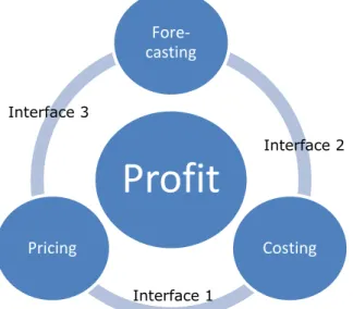
The highly competitive environment nowadays leads to a situation in which organizations are more and more focused in making profits. Concerning to profits, there are certain aspects that need to be considered; the cost incurred, the price asked and the quantity sold. The way that those entities behave is usually covered by a great uncertainty. Estimating this demand, setting the prices and defining the costs are subjects which are often explored in scientific literature, and it can be assumed that those research areas are related as well. The purpose of this report is therefore to investigate the interface between those three concepts and to bring a framework for managers who want to make a decision in either of the subjects involved.

However, the uncertainty inherent to the competitive environment has made demand estimation a difficult task to perform. Forecasting the demand is a common process in many organisations, but no matter how well it is done it will never represent the exact future. Nevertheless, there exist several forecasting methods which can provide different results which all have their own advantages, disadvantages and feasibilities. The biggest challenge is about picking the proper method.

One of the fields that can be seen as either an advantage and as a disadvantage of forecasting is the cost involved. The way that a firm assesses the cost has a significant impact on decision. In addition, the way that the cost is allocated is directly related to the cost information which is used all over the organisation. In general it can be said that no matter which approach will be used, the total cost is the same. Yet, the costing method chosen does affect the cost per unit

produced.

Cost information is typically used to make the most profitable decision

concerning to setting prices. In the broadest sense, there exists two ways of categorising pricing strategies, namely: cost and market-based methods. This are two extremes and each strategy can be found somewhere in between them. To test the assumption that the methods (pricing, costing and forecasting) are related, a literature review was performed. A considerable challenge faced by the researchers was the lack of scientific material when it comes to the interfaces. Where the fields between two of the subjects are partly investigated, the interface between all three of them is not investigated at all.

In this report, a model was created in which three different interfaces between the subjects were combined into a comprehensive one. After the analyses, it could be concluded that the methods investigated are not related to each other on a direct level. On the other hand, the outcomes of the methods affect each other directly. In the easiest way, it can be said that the price of a product affects the demand of that particular product. In its turn, the demand of the product affects the unit cost, which affects the price again.

However, it is also concluded that each method is related to the outputs of the other ones. In general, it can be said that those outputs are usually used as an input for the other methods. This was all summarised in the main research model developed in this report.

(5)

Key words

(6)

1. Introduction

1.1 Background

Production environments are flexible systems which are always changing. Over time, there have been two extremes in the way that production operations were managed. Historically, the craftsmanship was the first method used. This was a period in which one craftsman processed raw material and then forwarded the product or component to the next representative in the production process, and this went on until the product was completed (Bellgran & Säfsten, 2008). In addition, the craftsman owned all the tools and had control over the entire

production process (Berner, 1999). After a while the demand increased, and with the industrial revolution the craftsmanship became inefficient, requiring new methods. In such a context Ford, by using the scientific management

methodology combined with the idea of continuous flow as well as

inter-changeable parts, introduced the mass production concept (Bellgran & Säfsten, 2008). Mass production is a very popular research subject since the 1920s (Tolliday, 1998a) and appeared to be a solution for the inefficiency problems related to previous methods. Concerning the costs, the mass production led to enormous reductions in terms of unit cost due to higher production volumes. Consequently, Ford was able to sell its products at extremely low prices which, in turn, led to an enormous market share (Tolliday, 1998b). However, this method required large batch sizes and the system was based on anticipated sales

(Tolliday, 1998b), which led both to serious problems for Ford as well as the financial crisis of the 1920s. Big business and farmers assumed that the crisis was a consequence of overproduction and consumers and union bodies thought that the depression was a result of low purchasing power (Nyland & Heenan, 2005). Although those two perspectives are rather different, they do show that the crisis of the 1920s was characterized by an overproduction and low market demands. It is questioned that if demand forecast methods were applied the consequences might have been softer.

Now-a-days, however, the situation on the global market has changed and pure mass production is no longer suitable. Globalization had not just linked people from different places but also increased the competition. In the 1960s and 1970s the call was always for improving productivity (Lines, 1996), but after many technological innovations the production capacity overrun the customer’s demand (Lines, 1996). Consequently, this led to the fact that the customer’s requirements increased and that, for instance, lead times had to be reduced (Lines, 1996). In order to fulfil these demands organizations started to build inventories, planning and forecasting activities became more important (Lines, 1996; Fildes, 1988). Within manufacturing areas it is common to build short term forecasts (usually up to six months) in order to define what to manufacture, ship and stock. (Lines, 1996). Because of the costs related to these aspects, improved demand forecasting accuracy can lead to significant monetary savings. In

addition to that it can also lead to greater competitiveness, enhanced channel relationships, customer satisfaction (Moon, Mentzer, & Smith, 2003) and, consequently, higher sales figures. This has shown the importance of the

relationship between costs and forecasting, but personally we also think that the relation with price management can be interesting for many organizations. Like mentioned by Frontistis and Apostolidis (1987), the multiplicity of company

(9)

endeavours to gain customers, to search for new products and to anticipate the actions of competitors makes forecasting a must (Frontistis & Apostolidis, 1987). Although this does not clarify how forecasts and price management are related, it shows that it is clearly connected.

It is assumed that the lack of knowledge about the relationship between

forecasting, cost- and price management, leads to inefficiencies in the decision making process for many organizations. Although sometimes all the knowledge is available, it is usually not centralized. This report aims at fulfilling this demand by investigating the subject and creating a comprehensive framework that can be used by management.

1.2 Purpose and Aims

Forecasting, cost management and pricing policies are topics which have been deeply investigated over time. In general, managers who are involved with shop floor activities have limited knowledge about how a forecasting method can affect the cost management and price policies. Often, it is assumed that those three subjects are correlated to each other, but there is still a lack of research on these interfaces. In the report this assumption will be tested and, as an outcome, the company-wide knowledge about these subjects will be combined in a framework that can be used by management.

1.3 Delimits

Pricing, forecasting and costing are three different subjects which are all widely explored. Sometimes the border of each subject is unclear and overlapping with other research fields. In order to clarify the use of these terms and to guide the research project, some delimits were defined.

First of all, the report is written with an organisation as a point in the middle. When the terms price or pricing are used, this means that it is the price that the company (in which the manager works) set. In other words, it is not the price for product bought and this is considered as a cost.

Secondly, when forecasting is being described it discusses demand forecasts. Although other kinds of forecasts can be interesting as well, they are excluded from this research and left to other researchers.

Finally, the costing methods investigated are based on an accounting

perspective. Often, managers base their decision on accounting report or on accounting information and therefore other kind of perspectives about cost, like economical, will be excluded.

(10)

1.4 Outline

The following report is divided in a set of chapters in order to provide a clear and rational explanation about the main subject.

Chapter 1 - The first chapter aims to describe the current situations

(background), to introduce a problematic issue to be investigated (the research problem), state consistent reasons for investigating such area, and set the research limits.

Chapter 2 – This chapter concerns to the theoretical background. The main

pricing, costing and forecasting concepts are presented in order to provide a better understanding about the analysis performed and the conclusions reached. At first, the most used terms are brought up and then the main methods used nowadays are explained. A decision making part was also included due to its relevance when it comes to the analysis of those the subjects.

Chapter 3 – The research methodology employed in this studied is elucidated in

this chapter. It explains the research methodology adopted in order to provide a scientific credibility and validity for this work.

Chapter 4 – The cost and price relationships are analysed in this chapter. At

first it addressed two important questions (Are those methods related? If so, How related are they?). This chapter aims to answer those questions by analysing the relationship in two different perspectives; organizational and supply chain.

Chapter 5 – The costing and forecasting relationships are analysed in this

chapter. Following the same structure used in the previous chapter, two questions are addressed (Are those methods related? If so, How related are they?), and this chapter aims to answer those questions by analysing the relationship in the same way (organizational and supply chain perspective).

Chapter 6 - The price and forecasting relationships are analysed in this chapter.

Following the same structure used in the previous chapter, two questions are addressed (Are those methods related? If so, How related are they?), and this chapter aims to answer those questions by analysing the relationship in the same way (organizational and supply chain perspective).

Chapter 7 – This chapter analyses the links among the core research subjects:

pricing, costing and forecasting.

Chapter 8 – In this last chapter the researchers present their finding and

conclusions about the topic. In addition, topics for further researches are suggested.

(11)

2. Theoretical Background

2.1 Decision Making Process

The theory about the decision making process is an interesting subject. Every manager is in fact some kind of decision maker and usually the performance is formed by (the results of) the choices made (Vroom, 1973). Decisions are made all the time, although sometimes unconsciously. It is a subject that is relevant for many business areas and, in this situation, it can be used to define the optimal way of defining new policies concerning forecasting, cost and price management.

2.1.1 Decisions in Organisations

In order to be able to help management in making decisions concerning forecasting, cost and price management it is essential to define what a

management decision actually is. In the literature, several definitions have been used, but for the purpose of this report Ofstad’s version is of great relevance: “To say that a person has made a decision may mean:(a) that he has started a series of behavioral reactions in favor of something, or it may mean (b) that he has made up his mind to do certain action, which he has no doubts that he ought to do. But perhaps the most common use of the term is this: ‘to make a

decision’. (c) To make a judgement regarding what one ought to do in a certain situation after having deliberated on some alternative courses of action.”

(Ofstad, 1961)

This means that decisions by management should be made in a systematic and logical way, have clear objectives and should analyze several alternatives that could fulfil the requirements. However, the decision makers of today face problems that are increasingly complex and that are often interrelated (Diehl & Sterman, 1995; Moxnes, 2000; Sterman, 1989). The task of management is to analyze the situation and to make the right decision at the right time.

This kind of decisions can usually be divided into different categories. One possible way of characterizing decisions is, for instance, by dividing them into decisions that deal with the short term and those that affect the long term

aspects (Vaught & Walker, 1986). Short-term decisions usually relate to the day-to-day businesses and operations, while long-term decisions generally concern those activities that affect the organization’s destiny by, for instance, setting up new policies (Vaught & Walker, 1986). Another method of categorising them is by their occurrence. Decisions that are recurring or that are routines are

considered to be of one kind, while the ones that are non-recurring can be considered of a second category. Those recurring decisions are usually made by lower management, while the non-recurring are typically made by middle and upper management (Harrison & Pelletier, 2000).

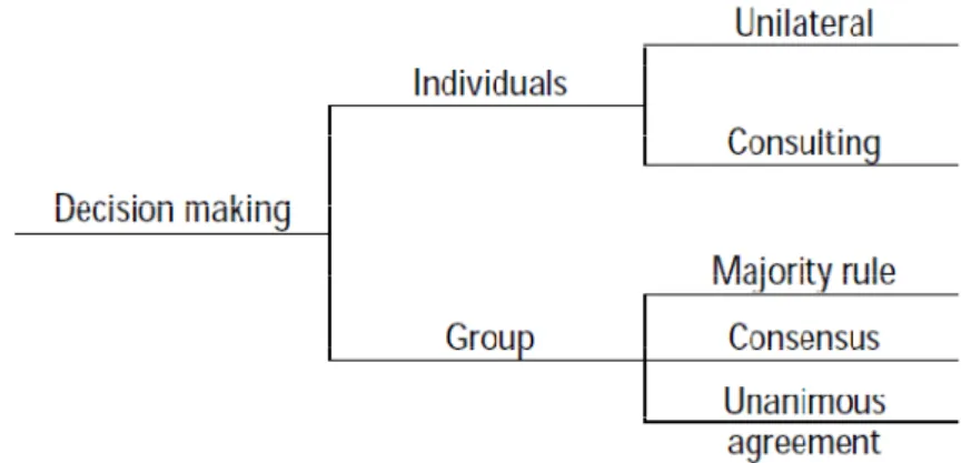
There are also two different ways of decision making, namely individually or within groups (Wright & Goodwin, 2008); although there are also several sub-levels in between, like can be seen in the next figure (Kessler, 1995).

(12)

Figure 1: Decision Making (Kessler, 1995)

It can be said that, in the figure above, the decision that will be made moves down from a situation in which there is just one decision maker to a situation in which an entire team makes it unanimously. Generally, it can also be said that decisions are stronger when there are more people involved in the process (Kessler, 1995). This means that the willingness, under e.g. personnel, to follow the outcome of a decision is the highest when many persons feel like they

contributed to it. For managers it is therefore recommendable to include many employees in decision making processes. In order to make a decision, it is required that the decision makers have the right amount of power and

authorities and are able to make sure that resources are allocated as required (Hayes, 2007; Osland, Kolb, & Rubin, 2001). In other words, this means that the decision making team should have the right power/authority, responsibility and budget to make the desired decision.

The effectiveness of decisions can usually be defined by: 1) the quality of the decision, 2) the time required to make it, and 3) the commitment of

subordinates in executing it (Vroom, 1973). This is partly confirmed by Harrison and Pelletier (2000) who say that the success of the decision can be measured by the acceptance of the external environment.

2.1.2 Decision Making Processes

At the moment, most persons who work with decision making use mainly simple hierarchic structures consisting of a goal, criteria, and alternatives (Saaty & Vargas, 2006). Although this fulfils all the criteria that Ofstad included in his definition, it raises the question about what the most effective method actually is. According to Rausch there is no comprehensive framework or collection of guidelines, that is widely understood and accepted, which can be used to make managerial decisions (Rausch, 1996). However, since one of the main purposes of this report is to guide management in making decisions, it is still advisable to use one systematic methodology. Therefore, two possible methods are described further down in this section.

The managerial decision-making process

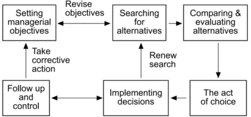
“The managerial decision-making process” (Harrison & Pelletier, 2000; Harrison, 1996) is a model that describes the different phases in a decision making

process. As it describes, the model from figure 1 consists out of six different areas that are all interrelated and form a dynamic process.

(13)

Figure 2: The managerial decision-making process (Harrison, 1996; Harrison & Pelletier, 2000) Hereby the decision making process starts with setting the managerial

objectives. This managerial objective is within definitive time and cost constraints and usually originates from an external need or opportunity (Harrison & Pelletier, 2000). Afterwards, the manager usually starts to search for alternatives,

compares and evaluates the different alternatives and then creates an action plan for implementing it. The evaluation and comparison of the different

alternatives is greatly influenced by the personal characteristics of the person or the team that is in control. A clear characteristic that affects the final decision is given by Harrison and Pelletier (2000) who explain that the risk acceptance or avoidance of a person or (project) team is often the most important decisive factor. After the decision is made and a plan of action has been formed, the decision should be actually implemented and followed up and controlled.

Since the managerial decision making process is a dynamic procedure, it is also possible to go back several times. This means that after analysing the results of a step, the decision maker can go back and try to get to a better input for that particular part of the process.

The Rational Decision-Making Process

A second approach that can be used to make strategic decisions, consists out of the following ten different steps.

1. Recognize and define the problem.

2. Identify the objective of the decision and the decision criteria. 3. Allocate weights to the criteria.

4. List and develop the alternatives. 5. Evaluate the alternatives.

6. Select the best alternative. 7. Implement the decision. 8. Evaluate the decision. (Osland, Kolb, & Rubin, 2001)

Based upon this theory, Herbert Simon won a Nobel Prize for his theory of bounded rationality (Osland, Kolb, & Rubin, 2001). Although it is often

questioned (Kerr, 2007), bounded rationality is still a popular research subject. The concept is based on the idea that, like the name already suggests, there are bounds on the rationality of persons. In the economics the main idea is often that persons will try to make the optimal decision (Brown, 2004). However, Simon’s theory objects that by giving a philosophy that suggests that managers

(14)

‘sacrifice’ rather than ‘maximise’ while making decisions (Simon, 2002; Brown, 2004; Osland, Kolb, & Rubin, 2001). This means that managers can only make decisions with the knowledge and information which is available for them, and the decision will be made as soon as the expected result is ‘acceptable’. Osland, Kolb and Rubin (2001) explain this with an example about internet. As they describe it, it is usually impossible to find an optimal website, so persons stop searching as soon as their result ‘satisfies’ their needs or purposes.

Simon (2002) gives hereby several procedures to transform an intractable decision into a tractable one, which say that managers should “look at

satisfactory choices instead of optimal ones”, “replace abstract, global goals with tangible sub-goals, whose achievement can be observed and measured”, and split up the work between different specialists and coordinate their work instead (Simon, 2002). All of this is included in his bounded rationality theory.

(15)

2.2 Demand Forecasting Methods

Predicting the future is always a challenging task. Through the years people have been aiming to foresee future events in order to clarify their main doubts. Who is going to be the next president and which team is going to be the next champion are examples of questions addressed nowadays. In fact the uncertainty by itself affects people’s life and for that reason there is an increasing attempt to improve the forecasting methods.

The following chapter is dedicated to present the main demand forecasting

methods used in enterprises nowadays. At first, a brief elucidation about demand instability will be presented in order to provide a better understanding about the subject. Afterwards, the main demand forecasting methods will be presented in combination with their advantages, disadvantages, accuracy and feasibility.

2.2.1 Demand

The demand concept is extensively explored in the microeconomics literature. Generally demand is analyzed together with supply because there are strong connections among those subjects. Depken (2005) says that the demand of a product is related to its price at a given period of time. At a glance such

relationship seems simple and easy to understand, but there is a big difference between the theory of microeconomics and the practice. To analyze demand (and other aspects of the economy), economists assume that everything in the

economy is held fixed. However, in practice, just a few factors are truly fixed, which makes economy analysis a difficult task to perform (Depken, 2005). In order to understand the complexity of demand, and consequently their

relationship to supply, it is important to mention the elasticity concept. According to Depken (2005) elasticity measures the relative change in one variable in response to a relative change in another variable. There are two important elasticity concepts: price elasticity and demand elasticity. Demand elasticity is rarely discussed in the literature (Case & Fair, 2003), it assumes that the product’s price may drop as the demand for it arises. For instance, the oil and steel industries are heavily affected by this phenomenon. According to

Schotamus, Telgen and Boer (2009) it can be explained by increases in economy of scale and/or transaction costs. Price elasticity, on the other hand, is about the variation in demand when the price is changed (Kotler, Wong, Saunders, & Armstrong, 2005). Simply, it “measures the sensitivity of demand or supply of goods to percentage changes in the price of those goods (price elasticity)” (Harding & Long, 1998).

Demand is a complex subject because it can be affected by many factors. Krajewski and Ritzman (2002) categorize those factors in two main groups: external and internal factors. External factors are those which are beyond the managers’ control such as governmental policies, change in customers’

requirements, expansion or contraction of market share and so forth. Internal factors, on the other hand, are those related to internal decisions and therefore it is under managers’ control. For instance, price settings and advertising

promotions are probably set by the marketing department and it can affect the sales figures. Krajewski and Ritzman’s explanation is quite simplistic; in order to get a better idea about demand complexity it is necessary to look through

(16)

by price setting, disposal income of customers, expected future prices, the number of demanders and suppliers and, finally, the customer’s preferences (Depken, 2005).

By observing the demand figures for a specific period of time it is possible to identify some basic patterns:

• Horizontal - fluctuation of data around a constant mean;

• Trend - consistent changes in the mean of the series over time;

• Seasonal – repeatable pattern of change in demand depending on the time of the day;

• Cyclical - or less predictable gradual increases or decreases in demand over longer periods of time (year or decades);

• Random –variation in demand which is not possible to forecast. (Krajewski & Ritzman, 2002)

Those patterns are called times series and can be useful in understanding future trends.

Before choosing a forecasting method some important factors have to be taken into consideration. Krajewski & Ritzman (2002) mention three important decision criteria concerning forecasting:

• Level of aggregation - By clustering several similar products or services in a process called aggregation, companies can obtain more accurate

forecasts;

• Units of measurement - It can vary depending on the aim (volume demanded, expected earning in sales, expected cost, and so forth); • Forecasting horizon - Short (0-3months), Medium (3months- 2years),

Long (More than 2 years).

Asides the level of aggregation, the unit of measurement and the forecasting horizon (Krajewski & Ritzman, 2002), some other factors also have to be taken into consideration, such as: the stage of the product’s life cycle (Chamber, Mullick, & Smith, 1971), the availability of data (Baines, 1992), the accuracy desired (Barron & Targett, 1986), and the application for the forecasting method (Chamber, Mullick, & Smith, 1971). Jenkins (1976) summarized all factors which have to be considered and developed a 9 steps systematic procedure to guide users in their forecasting selection:

1. Analyse the decision-taking system — this involves describing all decisions affected directly or indirectly by the forecasts, so that it is clear what is required of the forecasts;

2. Define the type and timing of the forecasts in the light of knowledge about the decision system collected at stage 1;

3. Consider what factors influence the forecasts and should therefore be reflected in the forecasting technique; in other words construct a conceptual model of how the forecasts should be made;

4. Check the quality and availability of data — the forecasting technique may be limited by scarcity of data;

5. Decide the technique(s) that are to be used — this is sometimes thought to be all that forecasting consists of;

(17)

6. Appraise the likely accuracy of the forecasts — this is elaborated below in the section on recognising good and bad forecasts.

7. Decide how judgment is to be incorporated — this is described in greater detail below;

8. Implement the system — again there is more detail on this below, and 9. Set up a method for monitoring forecasts as they are used — this is done

with the aim of making improvements in the light of experience.

2.2.2 Forecast methods

There is a wide range of forecasting methods that can be used (Chamber, Mullick, & Smith, 1971), each has its advantages and disadvantages which makes them feasible for particular situations. Generally, they are divided in two groups: qualitative and quantitative methods. A prerequisite for quantitative methods is the historical data. With historical data on hands it is possible to identify demand patterns and consequently estimate future demands. The qualitative methods are used when historical data are lacking, and it relies in several sources of information in order to generate forecasts (Krajewski & Ritzman, 2002).

A common mistake among forecasters is the focus on the current product

portfolio and new product ideas already generated. However, one aspect which is usually not considered is the concept of customer expectations. In many

situations it is more interesting to figure out what is value to the customer rather than just forecasting demand for the current situation. Knowledge gained from this kind of forecasting can, for instance, be used in new product development and to gain a higher customer satisfaction. Most of the forecasting methods described later on can be used for both purposes of forecasting.

Qualitative methods

Qualitative forecasting methods are always used in situations where data is scarce. For instance, when a new product is introduced to the market qualitative forecasting methods might be the only possible alternative due to the lack of historical data. According to Chamber, Mullick and Smith (1971), qualitative methods aim to bring together all information available and judge it in a logical and systematic way in order to avoid biased judgments. The most cited

qualitative methods in the literature are: Sales-force estimate, Execute (or expert) opinion, Market research and Delphi method.

Sales-force estimates: Sales personnel are the members of the company who are in constant contact with customers and therefore an important source of

information. Sales personnel can be involved in forecasting because they probably are the persons within the company who know most about the customers’ behaviour. According to Krajewski and Ritzman (2002), the main advantages are:

• Sales is the group which is most likely to know which products or services customers will buy in the near future, and in what quantities;

• The information given is broken down in a way that can be useful for inventory management, distribution, and sales-force staffing purpose;

(18)

• The forecasts of individual sales force members can be easily combined to get regional and national sales.

However such approach has also disadvantages. According to Krajewski and Ritzman (2002) the main disadvantages are:

• Individual biases of the salespeople may taint the forecast; moreover, some people are naturally optimistic, others more cautious.

• Salespeople may not always be able to detect the differences between what a customer “wants” (expectations) and what the customers “needs” (requirements).

• If sales figures are used to measure sales performance, then sales personnel may underestimate their forecast.

Executive opinion: There are some situations in which forecasting a future demand requires a certain degree of expertise which is not internally available. For instance, estimating the demand of a new product for the market can be a challenging task due to the lack of a database. In such situation hiring an

“Expert” can be an option. In doing so, the opinion, the experience, and technical knowledge of one or more executives are used to overcome problems related to lack of internal expertise (Krajewski & Ritzman, 2002). Those kinds of

professionals are in better position than the company to prepare forecasts because they have more data available and forecast expertise (Kotler, Wong, Saunders, & Armstrong, 2005). The main advantage of this method is the easy access to this kind of professionals. On the other hand, hiring an “expert” can be very costly (Krajewski & Ritzman, 2002). Cost and forecast accuracy is a trade-off since highly skilled and experienced executives require high wages. At last, the accuracy for short, medium and long terms forecast depend on how skilled and experienced the executives are.

Market research: Is an approach in which a range of techniques is applied in order to get valuable information about customers’ behaviour, and consequently it can be used for forecasting purpose. The main idea behind market research is to obtain information directly from the customer, and the most used method for obtaining such data is the survey. Surveys are used when the purpose is to determine extent, dispersion, and relation between variables in a population (Williamson, 2000). Krajewski and Ritzman (2002) give us a hint of how to carry out a survey:

1. Design a questionnaire that requests economic and geographical

information from each person interviewed and ask whether the interviewee would be interested in the product or service;

2. Decide how to administer the survey: by phone polling, mailings, or personal interviews;

3. Select a representative sample of households to survey. This should

include a random selection within the market area of the proposed product or service;

4. Analyze the information using judgment and statistical tools to interpret the responses, determine their adequacy, make allowance for economic or competitive factors not included in the questionnaire, and analyse whether the survey represents a random example of potential market.

(19)

Market research has several advantages: it is a good method to identify turning points and it does not require any special computerized calculations (Chamber, Mullick, & Smith, 1971). In addition, the information gathered is so detailed that it can be used to identify and define marketing opportunities and problems. Moreover, market research enhances the communication within the company. However such tool has also disadvantages. It is a complex procedure which involves analytical techniques. If it is used incorrectly it may not provide usable information (Birn, 2004). Besides that, it can be costly and time consuming process (Chamber, Mullick, & Smith, 1971).

Market research can be used for short, medium and long-term forecasting, but according to Krajewski and Ritzman (2002) the accuracy decreases when the forecast horizon increases. At last, market research can be advocated to forecast long-range and new products sales (Chamber, Mullick, & Smith, 1971).

Delphi Method: In order to reach a high degree of accuracy the forecasting method requires several sources of information. Sometimes those sources are contradicting which might become a problematic issue within the company. Delphi is a research method to solve problems of divergence by reaching a consensus through several repeated rounds of questions (Williamson, 2000). So far it is the most well known method of eliciting and synthesizing expert opinion (Cooke, 1991). First of all, a monitoring group defines the main questions to be addressed and selects the group of experts who will be involved in the process. The respondents are just known by the monitoring group and the responses are kept anonymously. Secondly, the problem is presented in a questionnaire form and the group of specialists are requested to answer. Thirdly, the set of

responses is gathered in a panel and then sent back to the respondents; together with the median answer and the inter quartile range (Cooke, 1991). Consequently, the participants are requested to answer the same question, but now considering the given answers. The second and third steps are repeated until the consensus is reached. (Williamson, 2000).The respondents whose answer were outside the inter quartile are asked to justify (Cooke, 1991). According to Kahn (2006) the successive rounds is an advantage over other forecasting methods because it provides consolidated feedback to the

respondents and also increases the consensus among the experts. An additional advantage is the anonymity aspect which minimizes the effects of social pressure to agree with the majority, ego pressure to stick with your original choice, the influence of repetitive argument, or the influence of dominant individuals (Kahn, 2006; Munier, 2004). On the other hand, such method also has disadvantages. Delphi method is time consuming since it requires several rounds and each round might takes weeks to complete (Kahn, 2006; Krajewski & Ritzman, 2002).

Furthermore, the responses may be less meaningful than the response from a situation in which barely experts were involved (Krajewski & Ritzman, 2002). In practice, Delphi is advocated for developing long-range forecasts of product demand, new-product sales projection, and technological forecasting (Krajewski & Ritzman, 2002). The accuracy provided is almost the same for short, medium and long term forecasts, and it can also be used to identify turning points

(20)

Quantitative Methods

The quantitative methods are divided in two groups: time series analysis and causal models.

Time series Methods: “Time series analysis is the analysis of past behaviour or events across a number of (generally) even time periods in order to predict behaviour or events by extrapolation across the next few time periods” (Baines, 1992). For control and audit issues companies have to register and store

quantitative information. Through the years such information, if managed properly, can be an important source of information to help managers in their decision making process. However, pure quantitative information by itself is useless without being processed (Chamber, Mullick, & Smith, 1971). Time series method is the process of analysing past behaviour or events across a number of (generally) even time periods in order to predict behaviour or events by

extrapolation across the next few time periods (Baines, 1992). According to Chamber, Mullick and Smith (1971) time series analysis helps to identify and explain:

• Any regulatory or systematic variation in the series of data which is due to season ability - the “seasonal”;

• Cyclical patterns that repeat any two or three years or more; • Trends in the data;

• Grow rates of these trends.

Naive forecast: Is a time series method whereby the demand for the current period is used as a base for estimating the demand for the next period. If the demand changed between two last periods, the trend (the demand difference) is taken into account while calculating the next demand. For instance, if the

demand two months ago was 98 units and last month it was 104, the demand forecast for next month is 104+(104-98)= 110 units.

The main advantages are the low cost and simplicity. Such method works well when the horizontal, trend, or seasonal patterns are stable and random variation is small (Krajewski & Ritzman, 2002). However, the naive forecast requires a consistent demand database in order to check the patterns’ stability, which might be a problematic issue. In addition, it fails to foresee random events as well as identify the reasons behind changes in the patterns (Wacker & Lummus, 2002). Consequently, it is not efficient for identifying turning points. At last naive forecast is fairly accurate for short term forecasting and it is feasible for controlling inventory of low volume items (Chamber, Mullick, & Smith, 1971). Simple moving average: Is a method to estimate the demand by summing the demand of n periods and dividing the sum by number of periods (n). The number of n depends on the stability of the demand series, so large values of n’s are advocated when the series is stable and small when the demand series is instable (Krajewski & Ritzman, 2002). The accuracy decreases while the

forecasting term increases, so it is fair to good for short term, poor for medium term, and very poor for long term forecasting (Chamber, Mullick, & Smith, 1971). In order to reach a fairly good accuracy the demand has no pronounced trend or seasonal influences (Krajewski & Ritzman, 2002). An evident advantage is the easy calculation procedure, however a minimum of 2 years of sales history is needed (Chamber, Mullick, & Smith, 1971). In addition, such method has a very low cost due to its simplicity. On the other hand, simple moving average is

(21)

very poor when it comes to predicting turning points. Chamber et al (1971) advocated the simple moving average for inventory control of low-volume items. Weighted moving average: Is very similar to the previous forecasting method, but the difference is that weights are given for each period depending on its importance (Krajewski & Ritzman, 2002). In such method forecast demand is calculated using the following equation:

Where:

• F 1= Forecast • t = period of time • D = demand

• , , , … . weights for each period • n = number of periods

The number of periods (n) taken into the consideration and the weight for each period can vary depending on the time series. The most challenging task in such approach is to set the number of periods (n) as well as the weight for each period. By choosing the right number of periods and the weight for each period, the forecast error is minimized. Setting those parameters might be a time consuming task but it can be easily performed.

While dealing with weights two common terms are used in weighted moving average; front-weighted average confers higher weights for the most recent and current data, while the back-weighted average puts more value on the older part of the data (Larson, 2001). Weighted moving average is simple and inexpensive to perform, however it requires a consistent demand database and it is inefficient to forecast demand turning points (Chamber, Mullick, & Smith, 1971). Finally, the accuracy is fair for short term, poor for medium term and very poor for long terms forecasting and it is advocated for inventory control of low volume items. Exponential smoothing: Is a sophisticated weighted moving average method that calculates the average of a time series by giving recent demands more weight than earlier demand (Krajewski & Ritzman, 2002). A period before the forecast is weighted with the highest value, which decreases exponentially as we move to earlier periods (Kazmier, 2003). In another words, the forecast demand is composed by the forecast of the previous period plus a forecast error.

Mathematically exponential smoothing can be expressed in the following way:

Where:

• F= Forecast this period • Ft=Forecast last period • =smoothing parameter

Exponential moving average has the advantage of simplicity and minimal data required, it just requires two periods (Henderson & Morton, 2000). Consequently, it is inexpensive to use and very attractive to firms that make thousands of

(22)

forecasts, since it only provide demand figures for the next period in the time series (Kazmier, 2003). In addition, as all time series methods, this one is not good for identifying turning points (Chamber, Mullick, & Smith, 1971). Finally, exponential moving average is advocated for production and inventory control (Chamber, Mullick, & Smith, 1971).

Box-Jenkins: Box-Jenkins is a complete and iterative technique in which a time-series is fitted in a mathematical model aiming at minimizing the forecast error. It is complete because it combines trend, seasonality, smooth autoregressive and spiked forecast-error terms (Hanssens, Parsons, & Schultz, 2001). It is iterative because it requires several attempts to fit the time-series in a model (Waddell & Sohal, 1994). Autocorrelation is defined by Salvatore and Reagle (2002) as a correlation of errors in different periods. For instance, first-order autocorrelation is when a error in a specific period is positively correlated to the previous period. The models range from Univariate (modelling a time series condition of its past) to multi-equation (modelling more than one time series as a function of all other series in the equation) (Henderson & Morton, 2000).

Box-Jenkins shares almost the same advantages as the exponential smoothing method; it is inexpensive and simple (Chamber, Mullick, & Smith,

1971).Although the underlying model is complex due to its composition, it is easy to interpret conceptually (Hanssens, Parsons, & Schultz, 2001). The main difference while compared with other forecasting methods is the use of

autocorrelation to improve accuracy (Waddell & Sohal, 1994). Autocorrelation provides useful information to identify data patterns which is helpful to

understand the demand behaviour. In addition, autocorrelation is useful to diagnose whether the model is adequate or not (Henderson & Morton, 2000). However, such approach might demand a certain degree of expertise for building and maintaining the model (Hanssens, Parsons, & Schultz, 2001). Furthermore, box-Jenkins demands a consistent database for building and updating the

existing model (Chamber, Mullick, & Smith, 1971). At last, the accuracy is high for short-terms forecasting and it decreases while the forecasting term is

increased, and such approach is advocated for short term forecast of cash balance as well as production and inventory control for large volume items (Chamber, Mullick, & Smith, 1971).

Causal Models

Causal model are sophisticated forecasting tools which express in mathematical terms, through models, the relationship among the variables. By knowing the cause-effect relationships, it is possible to reduce the uncertainty and therefore take more confident decisions (Wacker & Lummus, 2002). However, causal models are iterative which means that it needs to be revised constantly. There are a wide range of causal models, each one with its advantages, disadvantages and feasibility. Due to the fact that our research focus is demand forecasting, just linear regression and econometric models will be considered.

Linear regression: Is the most famous and used casual method (Krajewski & Ritzman, 2002). In such approach one variable (the dependent) is related to one or more independent variable by a linear equation expressed below.

(23)

Y= dependent variable X= independent variable a= Y-intercept of the line b= slope of the line

In forecasting, linear regression can be used to identify the relationship between demand (dependent variable) and an independent variable such as price,

advertising expenditures, disposal income of customers and so forth. Computer programs are generally used to calculate the values of a and b as well as the forecast accuracy.

The main advantage of linear regression over others casual model methods is the low cost. In addition, such method is very efficient for identifying turning points. Moreover, the accuracy achieved is generally very good for a forecast horizon shorter than 6 months and poor for long terms. However, the accuracy depends on the ability to identify relationships and an historical of several years is

necessary to obtain good and meaningful relationships. Finally, linear regression is advocated for forecast the sales by product classes (Chamber, Mullick, & Smith, 1971).

Econometric Models: Linking theory and reality is a common problem in economics. Due to the high degree of dynamism and complexity inherent to reality, there is a need to build and test theories constantly. Econometrics is an approach which combines economic theory, mathematics and statistical

techniques to test hypotheses and formulate new theories (Salvatore & Reagle, 2002). More than a theory builder tool, econometrics can also be used to

estimate numerical coefficients of economic relationships, which is essential in decision making, and forecast events (Salvatore & Reagle, 2002).

Concerning to the methodology, econometrics is a stepwise and iterative

process. It starts building a mathematical model based on the economic theory. The model is composed by an explicit stochastic equation which connects an economic variable (the dependent variable) to one or more independent variables (Salvatore & Reagle, 2002). Then, a systematic data collection is carried out in order to build a quantitative database for testing the model. Finally, the proposed model is tested using regression analysis. Economical and statistical aspects are taken into consideration in this step. Econometric criteria are taken into consideration in this stage (Salvatore & Reagle, 2002). As a possible outcome the model can be accepted or rejected. If the model is

rejected, a new model has to be built and submitted to the same process again until it reaches a desired acceptance (Henderson & Morton, 2000).

The main advantage of this method is that it provides cause-effect explanations of how related the variables are (Salvatore & Reagle, 2002). Such cause-effect relationships are extremely valuable for understanding what affects the outcome and consequently foresee future events. In addition, econometrics is excellent for identifying turning points, which is a differential while compared with the time series methods. However, the advantages gained by the method may well compensate for the extra costs incurred (Henderson & Morton, 2000). Econometrics is very costly because it requires a specialist to analyse the

quantitative information and incorporate expert judgment (Allen & Fildes, 2001). In addition, it is a time consuming process (Chamber, Mullick, & Smith, 1971).

(24)

As it was stated previously, it is an iterative process which might take several rolls and months until reaches a desired accuracy. In general, econometrics has a good accuracy; especially for medium terms forecasting when the accuracy achieved is higher. At last, econometrics is advocated for forecasting of sales by product classes (Chamber, Mullick, & Smith, 1971).

(25)

2.3 Costing Methods

Costing is an extensively studied subject which has taken the attention of economists, engineers, and marketers. Through the years, both academics and professionals of those areas have been striving to understand the mechanisms that affect the cost behaviour. So far, a lot of scientific work has been done, relevant conclusions have been reached but still this subject is not totally

understood. Based on the idea that managers take cost information into account in the decision making process (Hansen & Mowen, 1995; Kaplan & Cooper,

1998), understanding the cost behaviour is a must. This following section aims to present the fundamental knowledge necessary to understand the costing

methods relationship with pricing and forecasting. The main costing methods found in the text books are presented, as well as its advantages, disadvantages, and feasibility. In order to provide a better understanding about the subject, some terms will be introduced on beforehand.

2.3.1 Definitions in Costing

Due to its multidisciplinary aspect, cost is defined in many ways. Economists, for instance, use the concepts of economic, sunk and marginal cost. The first one is the value of the best alternative use of resources (Perloff, 2009). The next concept refers to the expenditures that cannot be recovered (Pindyck &

Rubinfeld, 2009). Marginal cost, at last, is the increment in cost that results from producing one extra unit of output and tells us how much it will cost to expand output by one unit (Pindyck & Rubinfeld, 2009). In fact, economists have a much wider perspective about cost than engineers. However, even for economists, the concept of costs is sometimes a source of complexity. Accountants, on the other hand, are more focused on allocating cost to the product and to write financial reports. Therefore they use mainly costing terms that also sound familiar to managers.

Engineers, especially those involved in production activities, are focused at the sources of costs rather than at cost allocation. The main sources of cost as well as some examples are displayed in the following table.

Cost types Examples Labour costs Wages Salaries Imputed costs Depreciations Interest charges Material costs Raw materials Indirect materials Costs of external services Transportation Repairing Costs of society Taxes Contributions Table 1: Cost types (Zulch & Brinkmeier, 1996)

Labour cost refers to the expenditures in workforce necessary to complete a particular task. Impute costs are those related to assets; it is not the money spent but a cost assigned for that. Material costs are the expenditures with purchase of materials (raw materials and consumables). Costs of external

(26)

services are those related to outsourcing. Finally, costs of society are

expenditures related to obligated governmental agencies and additional non-obligation expenditures, like charity and sponsorships.

A definition which is given from an accounting perspective says that cost is a cash or cash equivalent value sacrificed for goods, and services that are expected to bring a current or future benefit to the organization (Hansen & Mowen, 1995). Allocating cost to cost objects (products and services) is not an easy task to perform. Those which are easily and accurate allocated to the objects are called direct cost (e.g. direct material and direct labour). Indirect costs, on the other hand, are those which are neither easily nor accurately allocated (Hansen & Mowen, 1995). It is often known as overhead costs. In addition, accountants also classify the cost in terms of behaviour. Variable costs are those which change in proportion to changes in the related level of total activity or volume (e.g. direct material). Fixed costs, on the other hand, are those which remain unchanged in total for a given time period (e.g. salaries) (Horngren, Forster, & Datar, 2000).

2.3.2 Cost allocation methods

Job Order Costing: Costing allocation is, always a problematic issue. Although direct material and direct labour hour can easily be allocated, overhead cost requires allocation criteria. In the Job Order Costing approach overhead is distributed using an allocation base. In order to allocate the overhead cost it is necessary: to define the cost objects at first, then to identify the indirect costs, to choose an allocation base, and finally to allocate indirect cost based by use of the allocation base. According to Hansen and Mowen (1995) the allocation rate is generally the direct labour hours, but a different allotment base can also be adopted. Armstrong (2006) give some examples of overhead allocation cost bases commonly used, namely: machine hours, floor space and power consumed.

In general, Job Order Costing has the following characteristics:

1. The method require detailed postings of material requisitions, direct labour time tickets to many separate cost sheets, and a distribution of indirect manufacturing costs over several jobs (Crowningshield, 1969; Garrison, 1979);

2. It supplies more accurate and theoretically correct cost data, making costs for specific jobs more exact. Its clerical burden can be significantly reduced by the use of computers (Rushinek, 1983);

3. It provides management with two types of information: The cost of a particular job and the overall cost-effective information. The first one helps the manager to determine the price that should be charged, as well as the duration of the job. The second one determines the conformity of actual costs with budgeted standards (Copeland & Dascher, 1978).

When allocating costs with this method it is important to keep all relevant costs, including an overhead allocation, with a particular job until it is completed and sold. If the actual manufacturing overhead and applied manufacturing overhead are not equal, a year-end-adjustment is required (Webster, 2003). In Job Order Costing, similar products which were produced in the same way might have different cost (Rushinek, 1983).

(27)

Job Order Costing systems are mainly used when the company produces several different products, usually simultaneous, in each period (Berry, 2005). The cost object is usually a small quantity of heterogeneous products or services that can be produced as a single unit or even in batches (Garrison, 1979). The product is specially designed according to particular customer’s specifications, giving the product a high degree of customization (Berry, 2005). Consequently, it is largely confined to industries that make a product after a customer has placed an order which has certain specifications (Arnstein & Frenk, 1980). Examples of industries using Job Order Costing include machine tool manufacturing, furniture

manufacturing, shipbuilding, machinery products, printing, health-care service, aircraft industry, and construction. However, Job Order Costing is also becoming more common in manufacturing industries like electronics, due to an increasing demand for customized products (Horngren, Harrison Jr, & Bamber, 2002). Job Order Costing systems have the advantage of apparent cost absorption, which means that all the cost is allocated, including the overhead. According to Armstrong (2006) lowering prices to reach volumes sales might be a risky decision and there is a need to consider the fixed cost behaviour in a long term too. On the other hand, this method has disadvantages which have to be

considered while working with it. An allocation method based on a singular base can provide an inappropriate unit cost estimation if the allocation base is not properly chosen (Hansen & Mowen, 1995). In addition, such method requires a great amount of clerical work, which can demand a considerable effort

(Rushinek, 1983).

Process costing method: The idea of how process costing works is

straightforwardly connected to the company’s operational characteristics. Berry (2005) and Warren et all (2002) present evidences which link the company characteristics to the costing method. In order to better understand how the Process Costing method works, it is relevant to describe the environment in which such method is applied. In general, process costing is adopted by

companies which produce a large number of identical units that pass through a series of uniform production steps (processes) until its completion (Horngren, Harrison Jr, & Bamber, 2002). Companies working with process costing can produce a single or a variety of products using separate or even the same facilities (Rushinek, 1983). Foods, beverage and pharmaceutical industries are some examples of sectors that normally work with process costing method. Regarding to the method, the cost flow in a process costing system reflects the physical material flow (Warren, Reeve, & Fess, 2002). Direct material, direct labour and overhead costs are assigned to each step in a production process. In addition, there is a separate work in process inventory account for each process. The product incorporates its cost share in each process after being submitted to a transformation. Consequently, the product accumulates the cost as it moves through the processes until its completion (Horngren, Harrison Jr, & Bamber, 2002). Understanding the logic behind such method is not a difficult task to perform but accounting the unit cost might be very demanding. The reason for this difficulty, according to Berry (2005), is that in the various processes or departments there can be units in various stages of completion before and after the accounting period ends. More specifically, a manufacturing company may have to deal with one or more of the following situations:

(28)

• Units could be started and fully completed during the period;

• Units could be started during the current period but not completed until the next period;

• Units could have been started during the previous period completed this period.

An important source of information for accounting the cost is the production report (Warren, Reeve, & Fess, 2002). The production report is a document that mainly provides information about cost incurred (direct labour, direct material cost and overhead) and material used. Besides that such report provides

estimates of completion for each inventory category mentioned previously. The process cost system calculates the unit cost by adding the unit conversion cost to the unit material cost (Hansen & Mowen, Cost Management: Accounting and Control, 1995). The unit conversion cost is calculated by combining direct labour cost and overhead together and then dividing the sum by the total units

converted. Additionally, the material unit cost is computed by dividing the direct material cost by the total of units processed.

While calculating the unit cost there are several approaches which vary regarding to cost allocation but the most used approaches are: First-in-First-out (FIFO) and weighted moved average. FIFO assigns the conversion cost based on the degree of completion, considering uncompleted and completed units as different entities. The advantage of such method is that managers can use these current costs per unit to measure the efficiency of production during the month (Horngren,

Harrison Jr, & Bamber, 2002). On the other hand, weighted average method costs all equivalent units of work with weighted average of that period’s and the previous period’s per equivalent unit (Horngren, Harrison Jr, & Bamber, 2002). Hybrid Systems: There are some situations where the production process has characteristics that neither the Process Costing nor the Job Order Costing system is suitable to assign costs properly. For instance a particular footwear company produces batches of similar shoes with different materials for different markets. In this particular case the process costing method might be feasible to assign the conversion cost properly but not the material cost. In such situation a possible solutions for the allocation problem is to combine different costing systems in a single one: a hybrid system.

Hybrid costing systems combine characteristics of different costing systems in order to adapt the costing system to the production process characteristics. Hybrid costing systems are advocated for companies which produce batch of homogeneous products with different materials requirements (Hansen & Mowen, 1995). Wearing companies such as clothing, textiles, and footwear is an example of a sector which has batch production processes and adopts hybrid costing methods. In batch production process each unit of product is treated the same but different materials are required, thus moving it closer to a custom job order (Webster, 2003). The products might be visually identical but manufactured with different materials. Consequently, the conversion cost might be identical but the material cost differs from batches. So, Process Costing method is used to assign conversion cost and Job Order method to assign material cost (Berry, 2005). Joint Product Costing: Joint Product costing method is an approach designed especially for assigning cost to joint products. Joint products, according to Hansen and Mowen (1995), are products made from the same raw material,

(29)

which is divided in two or more products during the production process. A

butchering process is an example of Joint Product process. The raw meat is cut in different pieces which have different market value. Food industry, especially the ones related to meat packing and milk derivates, petroleum refining, chemical industry, and agricultural industry are other examples of companies that applies Joint Product Costing.

An important issue concerning to joint products is the concept of by-products. By-product is defined as a secondary product recovered in the course of

manufacturing a primary product and that has a relative minor sales value while compared to the main product. According to Hansen and Mowen (1995) by-products have the following characteristics, while compared to the main product:

1. By-product resulting from scrap, trimming, and so forth, of the main products in essentially non-joint-product types of undertaking;

2. Scrap and other residue from essentially joint-product types of processes; 3. A minor joint product situation.

Concerning to the costing method Joint Product Costing is basically used for accounting reasons. It has little or no use for decision making or cost control (Hansen & Mowen, 1995). Such method is applied because Joint Product companies are requested to present financial reports often and also because income tax law requires it.

Cost allocation is a difficult task to be done, and with Joint Product Costing is not different. Allocation cost requires an allocation base which is generally chosen in an arbitrary way. However, while dealing with Joint Product Costing, allocation for main products and by-products are done differently.

Activity- Based Cost (ABC): A typical characteristic of traditional costing methods is the use of a single allocation base. One allocation base has the advantage of simplicity and easiness. On the other hand, a single base allocation might provide unrealistic cost information, because it can underprice low volume,

custom products and overcost high-volume, standard products (O'Guin, 1991). It points to the conclusion that a single allocating base is insufficient in the

competitive environment nowadays; in most companies no single factor drives all indirect costs (Horngren, Harrison Jr, & Bamber, 2002). Since cost information is an important input for decision making, a more accurate costing method is

required in competitive environments

ABC is a unique costing approach that allocates cost in a rational and efficient way. More than just allocating cost, ABC is a costing system designed to provide information for decision making. Similarly to the methods mentioned previously, direct materials and direct labour are allocated in the same way. The difference is that ABC makes more effort to allocate indirect costs (Horngren, Harrison Jr, & Bamber, 2002). Organizational processes are first broken down into discrete processes and then into discrete activities and finally each activity is measured in term of cost and performance (Webster, 2003). The “breaking” process described previously is a necessary step for gathering corporative information required for setting the cost drivers. Cost drivers are the link between the cost and the object, therefore they are very important to understand ABC (Bengt & Loevingsson, 2005).

(30)

According to Berry (2005) the ABC allocation process can be divided in 7 steps: 1. Identify the activities that consume resources;

2. Identify and trace all direct cost to cost objects;

3. Identify the resource drivers for allocating overhead pools to each activity; 4. Identify the activity drivers to assign activity cost to cost objects;

5. Identify and allocate all overhead costs to activity;

6. Compute the total activity cost allocated to the cost object; 7. Use activity cost in decision making.

The first step is the most important; it aims to gather information which is essential for a proper cost allocation. The data collection can be carried out in different ways: through interviews, surveys, and flow charting (Berry, 2005). If the information collected is not accurate, it will affect the allocation output. Additionally, this step is time and resource consuming, therefore requires additional attention.

According to Kaplan and Cooper (1998) ABC application is guided by two simple rules: The Willie Sutton and the right diversity. The first one refers to the proportion of indirect cost over the total cost. Companies which have a high proportion of indirect costs might face problems with allocating cost. So, in this case ABC might be a solution to provide a better cost estimation. The second rule, “The right diversity”, is about the context’s degree of complexity in which the company is involved. The number of customers, the variety of products or services offered and the processes’ characteristics are aspects which affect the complexity of a enterprise. So, ABC cost is advocated for companies which face complexity in one or all those aspects mentioned previously.

ABC has the advantage of more accurate cost information for product costing, improved cost control (Clarke, Hill, & Stevens, 1999; Hussain, Gunasekaran, & Laitinen, 1998), more accurate allocation of indirect costs (Hussain,

Gunasekaran, & Laitinen, 1998), improved operational efficiency (Tayles & Drury, 2001), more accurate cost information for pricing (Clarke, Hill, &

Stevens, 1999; Tayles & Drury, 2001), preparation of relevant budgets (Tayles & Drury, 2001), modernization of cost accounting system in order to better depict costs (Hussain, Gunasekaran, & Laitinen, 1998) and improved business

processes (Tayles & Drury, 2001). On the other hand, ABC also has the

disadvantage of difficulties in identifying and selecting activities or cost drivers (Clarke, Hill, & Stevens, 1999; Hussain, Gunasekaran, & Laitinen, 1998),

problems in accumulating cost data for the new system (Hussain, Gunasekaran, & Laitinen, 1998; Tayles & Drury, 2001), time and resource consuming

implementation process (Gunasekaran, Marri, & Yusuf, 1999) prolongation of the time schedule of the adoption process and overrun of cost budgets (Tayles & Drury, 2001; Hussain, Gunasekaran, & Laitinen, 1998).