Improving movie recommendations through social media matching

(1)

Examensarbete

15 högskolepoäng, grundnivå

Förbättring av filmrekommendationer

genom social media matchning

Improving movie recommendations

through social media matching

Roman Kuroptev

Anton Lagerlöf

Examen: kandidatexamen 180 hp Handledare: Dimitris Paraschakis Huvudområde: datavetenskap Examinator: Johan Holmberg Program: systemutvecklare

Datum för slutseminarium: 2019-05-31

Teknik och samhälle

(2)

Sammanfattning

Rekommendationssystem är idag väsentliga för att navigera den enorma mängd produkter tillgängliga via internet. Då social media i form av Twitter vid tidigare tillfällen använts för att generera filmrekommendationer har detta främst varit för att hantera cold-start, ett vanligt drabbande problem för collaborative-filtering. I detta arbete adresseras istället hur top-k rekommendationer påverkas vid integrering av social media data i rekommendationssystemet. För att svara på denna fråga har en prototyp av nytt slag utvecklats inom processmodellen för Design Science. Systemet rankar om top-k rekommendationer baserat på resultatet av social matchning där användares Tweets matchas med nyckelord för filmer genom latent semantic indexing (LSI) similarity. Prototypen evalueras genom experiment som adresserar funktionalitet, noggrannhet, konsekvens och prestanda. Resultatet visar att mätetalen NDCG och MAP för top-k rekommendationer förbättras med social matching jämfört med att enbart använda collaborative filtering.

(3)

(4)

Abstract

Recommender systems are a crucial part of navigating the vast number of products on the internet. Social media, in the form of Twitter microblogs, has been previously used to produce movie recommendations, yet this has mainly been to solve cold-start, a common problem in collaborative filtering environments. This work addresses how top-k recommendations in a collaborative filtering environment are affected when augmented with social media data. To answer this question a novel prototype is developed following a design science process model. This system re-ranks top-k recommendations based on a social matching process where Tweets are matched with movie keywords through latent semantic indexing (LSI) similarity. The prototype is evaluated through experiments regarding functionality, accuracy, consistency, and performance. The results show that NDCG and MAP metrics of the top-k recommendations improve with social matching compared to only using the collaborative filtering algorithms.

(5)

(6)

Glossary

Top-k A ranked list of recommendations where k is the size of the list. Best

recommendations are in the top and less relevant items are further down in the list. Social-matching The process of matching all words in a user’s Twitter timeline with keywords for a movie.

Cold Start problem: A situation in collaborative filtering algorithms where not enough ratings, for either a user or an item, exist to be able to produce accurate

recommendations.

Corpus A collection of written texts.

Instance A working system created through design science. Also referred to as instantiation.

Artifact Models, methods, constructs, instantiations or design theories created through design science.

MAP A metric for evaluating all recommendations generated by a recommendation system. Takes the ranking of relevant items into account.

NDCG Similar metric to MAP used to evaluate the ranking of recommendations generated by a recommender system. But unlike MAP uses real-valued relevance instead of binary. Twitter-timeline A collection of all tweets posted by a Twitter user.

IMDb Internet Movie Database.

LSI Latent Semantic Indexing is a technique to analyze the relationships between terms in a document.

(7)

1. Introduction

Today, digital information is of abundance. More and more shopping, as well as consumption of media, has moved from real-world physical stores to the online arena. Whereas the limitations of physical shopping are set by how many articles can fit in the available physical space, online shopping and consumption of media, however, is not bound by these limitations. As of January 2018, a customer browsing the inventory of e-commerce mogul amazon.com was exposed to as many as 564 million items when accessing us marketplace (How Many Products Does Amazon Sell Worldwide – January 2018, 2018).

Recommendation systems play an important role in helping users find what they might like from this ever-increasing sea of information. By utilizing a user’s prior activity, a prediction can be made on whether he/she will like an item or not. According to research by McKinsey, as much as 35% of Amazon sales are a result of recommendations, and for the on-demand streaming service Netflix, an estimated 75% (MacKenzie, Meyer, & Noble, 2013).

Leading players in the digital arena, such as Amazon, YouTube and Netflix have demonstrated the value recommendation systems offer on both revenue and user experience. According to a 2015 paper published by Netflix, the company estimates their recommendation systems save up to as much as 1bn dollars per year. The authors of the paper state that “When produced and used correctly, recommendations lead to meaningful increases in overall engagement with the product (e.g., streaming hours) and lower subscription cancellation rates” (Gomez-Uribe & Hunt, December 2015).

The demand for well-performing recommender systems is high, making efforts of improving the underlying techniques which make these systems possible, relevant.

Another heavy player in the digital arena is social media. Here opinionated texts are regularly shared by millions of users on various topics and events. Safe to say, social networks are a rich source of users prior, and current opinions.

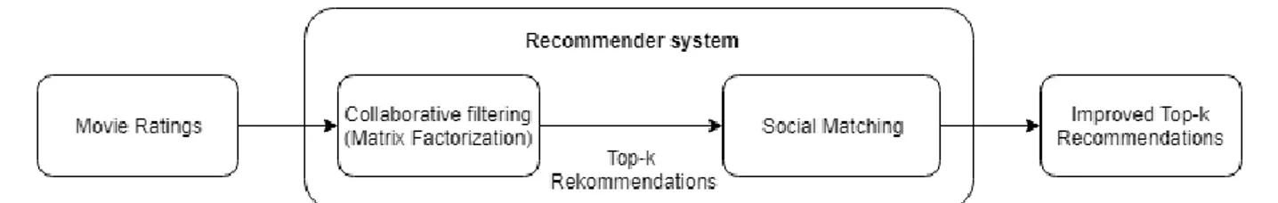
In this thesis, we propose SwarmBoost, a novel system integrating user data from Twitter into a recommender system environment. The proposed system, based on MovieTweetings (Dooms, Pessemier, & Martens, 2013), a dataset of Twitter user IDs and their corresponding movie ratings, is utilized to perform movie-timeline matching. SwarmBoost aims to discover if a Twitter users timeline can improve the recommendation results for two recommendation algorithm techniques. The system developed using the Design & Creation methodology in combination with experiments for evaluation tries to answer this by reranking user top-k movie recommendations.

Evaluation of the system is performed with a technical experiment to measure NDCG and MAP, two common evaluation metrics. Further, the artifact is evaluated based on four design science research criteria.

(12)

2

1.1 Research question

1. How can incorporating personal social media data, from Twitter, into a recommender system affect top-k recommendations produced by traditional collaborative filtering algorithms?

2. How does social matching effect metrics NDCG and MAP?

1.1.1 Objective

Design and implement an artifact that gives answers to our research questions. This Artefact is a recommendation system that uses social media in the form of Twitter to improve traditional recommendation algorithms. Taking the approach of improving collaborative filtering by reranking top-k recommendations using Twitter as a data source is to our knowledge a novel problem.

1.2 The structure of this thesis

The introduction is followed by a background to the topic and used techniques. It contains both relevant information on recommender systems as well as techniques used for movie-timeline matching and common metrics for evaluating recommender system performance.

Subsequently, a method section introduces the Design & Creation methodology and how it has been applied. The method also contains the proposed experiments and what they aim at evaluating from a Design & Creation viewpoint.

Design & Implementation describes the Artefact that was implemented from the design requirements established in the design phase.

The Results section presents the performed experiments in matrices accompanied by a brief explanation.

This is followed by an analysis discussion and conclusion of the results and ends with identified gaps for future work.

(13)

3

2. Background

2.1 Literature review

Although this work proposes a novel system by re-ranking top-k recommendations through social matching, studies augmenting collaborative filtering using Twitter data have been made. Similarly, studies showing the viability of latent semantic indexing (LSI) when applied to micro-blogs motivate it being the chosen technique for the timeline-movie matching procedure. In what manner Twitter has been utilized in collaborative filtering recommendation systems varies.

Nair, Moh & Moh (2016) utilize users Twitter profile to try alleviating cold-start, a problem often occurring in collaborative filtering environments. This problem occurs when a new user enters the system. When no previous ratings for the user exist, the recommender system does not know what to recommend to the user. Similar to this study, the authors model the Twitter-based dataset of MovieTweetings in order to create a collaborative filtering environment, combined with the Twitter timeline for 10 000 of the dataset’s users. Utilizing the plot of movies and their corresponding genre(s), a bag of words approach was used to compare each pre-processed user tweet with a movie plot to calculate cosine similarity. If the similarity was greater than the pre-defined threshold the genres for the movie were retained. In this manner, a list mapping each user and their corresponding frequency of genres were generated. To evaluate the system the list mapping users and top-k genres were used against the ratings for users in the MovieTweetings dataset. The metrics Accuracy (correct recommendations / total possible recommendations) and MAE (Incorrect recommendations / total possible recommendations) were used for evaluation. The results show an accuracy of 72%. Although taking a different approach, using genre, the study demonstrates the viability in matching user tweets with movie keywords to generate recommendations in a collaborative filtering environment based on the MovieTweetings dataset.

Alahmadi & Zeng (2015) similarly aim to alleviate cold-start in a collaborative filtering environment recommending movies. The proposed system, H-ISTS, is based on the idea that users tend to have high satisfaction when recommendations derive from friends or acquaintances. Hence the study does not consider the timeline of users, but the intricate relationships Twitter contains. The system utilizes the user’s connections on Twitter to perform multi-scale sentiment classification on tweets about movies. Thereafter so-called 'social trust' between the user and his/her connections is modeled by analyzing re-tweet actions and following/follower lists. Trust and sentiment values are then applied to the SVR model to create rating estimation. Several baselines are used in the evaluation phase.

LSI has been used to develop a plot-based recommender system to find similarity between the plot of user purchased movies and the plot of movies stored in a database (Bergamaschi, Po, & Sorrentino, 2014). They compared LDA and LSI for the best performance in the system. LSI showed the best results. Acosta, Lamaute, Luo, Finkelstein, & Cotoranu, (2017) studied the possibilities of using word2vec in sentiment analysis of Twitter data. Although their focus was not on LSI and similarity, they studied the possibility of finding term similarity between tweets. The results show that it was not efficient to use LSI to match single tweets to each other since tweets often were very limited and short which was not enough information for LSI and cosine similarity to find clear similarity results.

(14)

4

LSI was also used by Bansal et al (2016 ) to build a similar recommendation system as this work aims to do. The recommender system built by Bansal et al (2016 ) focuses on genre prediction to recommend movies based on matching tweets about a user’s one favorite movie with genre-specific movie data extracted from IMDB using LSI and Euclidean distance. The results indicate that predictions had a 70% accuracy. The difference between Acosta et al (2017) and Bansal et al (2016 ) is that the later used a Twitter data corpus consisting of a large number of tweets instead of single tweets which proved to be enough data for LSI and similarity matching. This shows that LSI can be efficient at finding document and term similarity between Twitter data and movie data if enough Twitter data is used.

2.2 Recommender systems

2.2.1 Overview

Traditionally there are two major categories within recommendation system (RS) techniques, content-based and collaborative filtering. Although taking different approaches, both share the common aim of predicting what items a user may like from a group of candidates in order to recommend relevant items to the user.

Two collaborative filtering techniques, Matrix Factorization (MF) and k-nearest neighbors (KNN) are used in this work as underlying algorithms for SwarmBoost. Even though this study has chosen collaborative filtering as its preferred technique, both content-based and collaborative-filtering are presented below in the hope of increasing the understanding of the overall concept of recommendation systems.

2.2.2 Content-based filtering

Content-based filtering relies on the attributes of items to filter out items from a set of candidates. It is based on the idea that if a user liked an item I, it is deemed likely that he will enjoy items with high similarity to that of I. It uses the attributes of the items to make its predictions, thus relies heavily on rich metadata. This makes it suitable for recommending items where this is the case, such as news articles and publications. To make its predictions it models the relationship between items and calculate their similarity (Aggarwal, 2016). Figure 1 below depicts the concept of Content-based filtering. Squares represent items in the recommender system. For instance, in the domain of e-commerce squares would here represent products sharing a high similarity.

(15)

5

Figure 1. Depicts the concept of content-based filtering.

2.2.3 Collaborative filtering

Collaborative filtering is based on the idea that similar users, i.e. users who have liked similar items in the past, probably have a similar taste. If let’s say user A and B have a high similarity of past ratings, an assumption can be made that items rated highly by B can be recommended to user A. Recommendations are generated from the utilization of matrix mapping users and items together. This ‘user-item matrix’ contains the behavior of each user, i.e. rating given to items in the past. Collaborative filtering is suited for environments where item metadata is limited, such as in the scenario of recommending music or movies. Generally, Collaborative filtering is more accurate than the content-based approach presented above (Koren, Bells, & Volinsky, 2009), although suffering from the often referred to the cold-start problem. This problem arises when a new user or item enters the system. When no past ratings are available, the system cannot generate accurate recommendations (Isinkaye, Folajimi, & Ojokoh, 2015).

In the case of this study, the cold-start problem was not deemed reason enough to choose a different approach due to the possibility of mitigating the problem by removing cold-start users from the used dataset. Collaborative filtering has also been heavily studied and improved and is today used in many large-scale recommendation environments motivating the choice of the technique as the choice of algorithm for our research.

Collaborative filtering is further divided into the two sub-categories of memory-and model-based techniques. One method from each of these sub-categories, used by SwarmBoost is presented below. Figure 2 depicts the concept of collaborative filtering.

(16)

6

Figure 2. Depicts the concept of collaborative filtering.

2.2.4 Model-based collaborative filtering using Matrix factorization

As users in a movie recommendation environment only rate a very small part of the items in the user-item matrix, it is common that collaborative filtering is affected by data sparsity. Matrix factorization has shown to be effective in mitigating this issue. This is achieved by reducing the user-item matrix into much smaller matrices to uncover latent features in the dataset.

The decomposition results in an association between each user and a user-factors vector, similarly each item gets associated with an item-factors vector. Predictions for how a user would rate an item can then be made by calculating the inner product. This work uses Weighted Matrix Factorization (Hu, Koren, & Volinsky, 2008), a modification of standard Matrix Factorization as it has shown good results for the dataset during initial experimentation.

2.2.5 Memory-based collaborative filtering using KNN

Memory-based collaborative filtering, often referred to as neighborhood-based filtering can be either user or item based. In this work the user- based approach is used and is, therefore, the one being described in further detail.

The user-based approach uses historical user rating data to compute the similarity between users to produce its item recommendations. To compute similarity the user-item matrix described under section collaborative filtering is utilized. Users with the high similarity of historical ratings are considered part of the same neighborhood. Recommendations for a user can then be made from items not rated by the user, but by users sharing that same neighborhood. The main advantage of this technique is its simplicity, making it easy to implement and debug. On the other hand, the disadvantage of this technique is that it is prone to data sparsity. This means that if no neighbors of a user have rated item I, it is not possible to recommend an item I to the user (Aggarwal, 2016).

(17)

7

2.2.6 Twitter as a data source

Twitter, with its 326 million active users as of 2018 (Twitter, 2018) is a rich data source. Opinionated texts are regularly shared by users on various topics and events.

A large extent of this data published on the site is public and available. Accessing Twitter programmatically is straightforward through the official Twitter API and established open-source libraries making it a common choice as a data open-source in both private projects and academic research. Although research using Twitter user data in a collaborative filtering environment has been done, it has mainly been to address the cold-start problem (Alahmadi & Zeng, 2015; Nair et al., 2016).

2.3 LSI

2.3.1 Vector space model

Natural language processing (NLP) is needed in the part of the recommender system that matches social data with movies. A document containing terms can be represented in several ways when it comes to NLP. A naive approach is the Bag of words model where terms are represented by an unordered list of the words (Zhang, Jin, & Zhou, December 2010). This model does not take word positions or semantic context into account. Only the occurrence of the term in the document is represented.

Tweet1 Tweet2 Tweet3

Term1 4 0 2

Term2 2 1 4

Term3 0 2 2

Figure 3. A Document term matrix consisting of four documents and three terms. The weights for each term are the frequency of occurrence.

A more complicated approach is the vector space model. Here the document and its terms are represented as multidimensional vectors where each dimension is a term found in the vector (Salton, Wong, & Yang, 1975). Figure 3 represents a document-term matrix. If the term exists in the document, its value in the matrix is non-zero. The document term matrix is one way to model a document, but it also suggests a different way. By modeling the terms as points in multi-dimensional term space the vector space model, which can be seen in figure 4, is created.

The value of a term is called weight and there are different ways to compute this weight. It can be a binary value representing if the term is present, it can be the frequency of occurrence or it can be a term frequency-inverse document frequency (TF-IDF) value. TF-IDF is a numerical statistic approach to setting weight and thereby significance for a term in a document (Salton, Wong, & Yang, 1975).

(18)

8

Figure 4. Graphical representation of vector space document matrix. Blue vector = Tweet1, Red vector Tweet2, Orange vector = Tweet3.

2.3.2 Latent Semantic Index

Latent Semantic Indexing is a mathematical statistical technique used to extract relations between documents and queries. (Deerwester, Dumais, Furnas, & Landauer, 1990)

Converting a document into a vector space representation is called indexing. After converting the document into a vector space document term matrix 𝐶 with frequency or TF-IDF weight for each term, the next step is to use singular value decomposition SVD.

This is a mathematical generalization technique used to reduce dimensionality in the document term matrix (Jagdale, Deshmukh, & S.G.Chodhary, 2016). First, the matrix is split into three different component matrices. One for each row 𝑉 (the terms), one for each column 𝑈 (documents) in derived orthogonal factor values and the third is a diagonal matrix containing scaling values. This diagonal matrix is needed to be able to reconstruct the original matrix by matrix-multiplication. By zeroing out some the lower order values in the diagonal matrix before reconstructing the matrix 𝐶′ the co-occurring terms come closer together and the resulting matrix 𝐶′becomes more compact and efficient than 𝐶.

(19)

9

2.3.3 Cosine similarity

Calculating the similarity between new queries and the document is done by adding the query as a new document and calculating the cosine similarity from the resulting query vector and the other vectors (Huang, 2008).

This is done by calculating the cosine angle of the two vectors. For example the cosine angle between two vectors in figure 4.

𝑠𝑖𝑚𝑖𝑙𝑎𝑟𝑖𝑡𝑦 = 𝑐𝑜𝑠 (𝛩) =

𝐴 ∗ 𝐵

|𝐴||𝐵|

Given two vectors A and B representing a document and a query, the cosine angle is calculated through dot product and magnitude of the vectors resulting in 1 as the maximum correlation, 0 when there is no correlation, and -1 if there is a negative correlation.

2.4 Evaluating recommender systems

The following section describes different metrics used to evaluate recommender system performance.

2.4.1 Item ranking prediction

Recommendation systems try to find items to recommend for a user. This can either be done through predicting a rating that a user would give or by predicting if the user would use the item at all. (Ricci, Rokach, & Shapira, 2010)

A list of prediction items can be assembled through item prediction. The ranking of the items in the list shows the highest deemed relevant items in the top.

Item prediction can be done either online or offline. In offline prediction, a data set consisting of usage history is collected and used. One user is selected and some of the usage history is hidden. The recommender system is then asked to predict the items that were hidden. With the items in the history that are not hidden as input, the recommender system tries to predict the hidden items.

In the offline scenario, it is assumed that items not in the collected dataset are items the user is not interested in, even if the user potentially would have been interested but never knew about the item.

The following section describes the Mean average precision (MAP) and Normalized Cumulative Discounted Gain (NDCG). Two metrics from information retrieval that are used to evaluate the ranking of the predicted items.

(20)

10

2.4.1.1 Mean average precision

Mean average precision uses both precision and recall. (Manning, 2008)

Precision is the amount of correct recommended items (true positive) divided by the

amount of all recommended documents (sum of true positive and false positive). This metric is used to show the probability of correct items recommend that are relevant to the user’s preference. In other words, how many of total recommended where correct.

Recall is the amount of correct recommended items (true positive) divided by the sum of

all correct items (true positive) and all false negative items. This metric is used to show the probability of a relevant item being recommended by the system. In other words, how many of the total possible correct items were recommended to the user.

Average precision considers the ranking order in the recommendation list. This is achieved by plotting a curve where precision 𝑝(𝑟) is a function of recall.

𝑘 is the rank of the item in the list. 𝑛 is the number of items in the list, 𝑃(𝑘) is precision at cutoff 𝑘 in the list 𝑟𝑒𝑙(𝑘) is an indicator function of the item at 𝑘 is relevant.

𝐴𝑣𝑒𝑃 = ∑ (𝑃(𝑘) × 𝑟𝑒𝑙 (𝑘))

𝑛 𝑘=1

𝑛𝑢𝑚𝑏𝑒𝑟 𝑜𝑓 𝑟𝑒𝑙𝑒𝑣𝑎𝑛𝑡 𝑑𝑜𝑐𝑢𝑚𝑒𝑛𝑡𝑠

Mean average precision is the mean of the average precision scores for all item recommendations for all users observed when evaluating the recommender system. (Manning, 2008)

𝑀𝐴𝑃 = ∑ 𝐴𝑣𝑒𝑃(𝑞)

𝑄 𝑞=1

𝑄

2.4.1.2 Normalized Cumulative Discounted Gain

Normalized Cumulative Discounted Gain NDCG is an information retrieval method that is used to measure the correctness of the ranking produced by a recommendation system. (Järvelin & Kekäläinen, 2002).

Cumulative gain is a predecessor to Discounted cumulative gain.

Cumulative Gain at p = CG_p = ∑ rating(i)

p

i=1

Where 𝑟𝑒𝑙 𝑖 is the graded relevance of the result at position i.

Cumulative gain is a measure of the sum of graded relevancies. It does not take the ranking

of the results into consideration.

Discounted cumulative gain (DCG) takes the ranking of the results into consideration by

(21)

11 𝐷𝑖𝑠𝑐𝑜𝑢𝑛𝑡𝑒𝑑 𝐶𝐺𝑝= 𝐷𝐶𝐺𝑝= ∑ 𝑟𝑎𝑡𝑖𝑛𝑔(𝑖) 𝑙𝑜𝑔2(𝑖 + 1) 𝑝 𝑖=1

DCG accumulated at a particular rank position 𝑝

To acquire a measure that is not only relevant for one prediction list and one correct result query the DCG need to be normalized to a value between 0 and 1.0. This normalized discounted cumulative gain (NDCG) is achieved by producing a maximum possible DCG through position 𝑝, an ideal DCG (IDCG) and dividing the produced DCG with the IDCG.

𝐼𝑑𝑒𝑎𝑙 𝐷𝐶𝐺

𝑝

= 𝐼𝐷𝐶𝐺

𝑝

= ∑

𝑟𝑎𝑡𝑖𝑛𝑔(𝑖)

𝑙𝑜𝑔

2

(𝑖 + 1)

|𝑅𝐸𝐿| 𝑖=1 𝑁𝑜𝑟𝑚𝑎𝑙𝑖𝑧𝑒𝑑

𝐷

𝐶𝐺_𝑝= 𝐷𝐶𝐺𝑝 𝐼𝐷𝐶𝐺𝑝

(22)

12

3. Method

3.1 Design creation methodology

The main research method used for answering the research questions stated earlier is Design and creation since all of our research questions can be answered through design and creation of a recommender system artifact through proof of concept demonstration and different evaluation metrics experiments.

Peffers, Tuunanen, & Rothenberger, (2007) define the purpose of Design research as "Design science creates and evaluates IT artifacts intended to solve identified organizational problems.”(p.49) The field of design research has several proposed processes models to apply for design research. Archer, Eekels, J. Roozenburg, and Hevner all propose different process models with varying degrees of details and steps (p.53). But they all share similarities.

Peffers, Tuunanen et al (2007) propose a unified methodological guideline process that is a result from studying previous design research process models. By applying the model on four case studies the proposed process model is proven efficient and versatile. The process model itself consists of six different activities with four different entry points into the process depending on what is most applicable.

Figure 5: The Design & Creation unified methodological guideline process.

Source: (Peffers, Rothenberger, Tuunanen, & Vaezi, 2012)

In the following section, each Activity is described accompanying a small description of how the activity was applied in the used research method. The process model is applied in a waterfall sequence without iteration since enough results were achieved. A problem-centered entry point was most applicable since the nature of the research question and objective of the research was centered around the problem of integrating social media into recommender systems.

(23)

13

3.1.1 Activity 1

Description

“Problem identification and motivation. Define the specific research problem and justify the value of a solution. [...] Justifying the value of a solution accomplishes two things: Motivates the researcher and the audience of the research to pursue the solution and to accept the results and it helps to understand the reasoning associated with the researcher's understanding of the problem” (Peffers, Rothenberger, Tuunanen, & Vaezi, 2012).

Application

The problematization identified in Activity 1 is the following:

Recommendation systems are an important part of revenue generation and user experience. The growing number of items in the e-commerce market creates a need for the best possible recommendation system to maximize and ensure revenue generation for the businesses and to ensure the best possible service and user experience for customers.

Cookies and browsing history are widely used in e-commerce recommendation systems but social media activity is an untapped source of user information when it comes to recommendation systems. Extraction of useful user information from a user’s social media posts is an uncomplicated way for a user to give more information about their preferences to a recommendation system. Much research has been done on applying social media to collaborative-filtering based recommender systems for alleviating the cold-start problem, yet research focusing on improving collaborative filtering performance is uncommon.

3.1.2 Activity 2

Description

“Define the objectives for a solution. Infer the objectives of a solution from the problem definition and knowledge of what is possible and feasible. The objectives can be quantitative, such as terms(?) in which a desirable solution would be better than current ones, or qualitative, such as a description of how a new Artefact is expected to support solutions to problems not hitherto addressed. “ (Peffers, Rothenberger, Tuunanen, & Vaezi, 2012).

(24)

14 Application

Relevant objectives defined during Activity 2 are the following:

Creating a recommendation system that uses personal social media data for a user in the recommendation process in a way that improves traditional existing recommendation systems. This is both a qualitative and quantitative objective since the fact that the system uses social media data is qualitative and the objective of actually improving existing recommendation system results is a quantitative objective.

3.1.3 Activity 3

Description

“Design and development. Create Artefact. Such Artefacts are potentially constructs, models, methods, or instantiations. Conceptually, a design research Artefact can be any designed object in which a research contribution is embedded in the design. “ (Peffers, Rothenberger, Tuunanen, & Vaezi, 2012).

Application

During activity 3 the Artefact that is used to fulfill the objectives of activity 2 is designed and a prototype is implemented to be used as proof of concept. Further design requirements and design decisions are presented in the Design phase section. The Implementation itself is presented in the implementation section.

3.1.4 Activity 4

Description

“Demonstrate the use of the Artefact to solve one or more instances of the problem. “ (Peffers, Rothenberger, Tuunanen, & Vaezi, 2012).

Application

To demonstrate the Artefact as described in Activity 4 the system is used in an experiment scenario with MovieTweetings, a dataset including movie ratings with IMDb IDs for the movies and Twitter user IDs. The dataset is split chronologically in order to predict user ratings and get results relevant to the objectives defined in Activity 2.

(25)

15

3.1.5 Activity 5

Description

“Evaluation. Observe and measure how well the Artefact supports a solution to the problem. This activity involves comparing the objectives (so we need to define this in objectives) of a solution to actual observed results from use of the Artefact in the demonstration. It requires knowledge of relevant metrics and analysis techniques. Depending on the nature of the problem venue and the Artefact, evaluation could take many forms. It could include items such as a comparison of the Artefact's functionality with the solution objectives from activity 2, objective quantitative performance measures such as budgets or items produced, the results of satisfaction surveys, client feedback, or simulations. It could include quantifiable measures of system performance, such as response time or availability. “

(Peffers, Rothenberger, Tuunanen, & Vaezi, 2012).

Application

Evaluation is performed in order to discover if and how well the proposed Artefact solves the proposed problem. Four of the terms presented by Hevner (2004), deemed most relevant, were selected to evaluate the instance. The following were selected: functionality, consistency, accuracy, and performance. What each of them denotes is presented in section 3.3.1.

A common evaluation technique in DS research, technical experiments are used for their evaluation (Peffers, Rothenberger, Tuunanen, & Vaezi, 2012). The experiments are also performed on different underlying collaborative filtering algorithms and randomization. The experiments and what they aim to evaluate is presented in greater detail in section 3.3.2.

3.1.6 Activity 6

Description

“Communicate the problem and its importance, the Artefact, its utility and novelty, the rigor of its design, and its effectiveness to researchers and other relevant audiences such as practicing professionals, when appropriate. In scholarly research publications, researchers might use the structure of this process to structure the paper, just as the nominal structure of an empirical research process (problem definition, literature review, hypothesis development, data collection, analysis, results, discussion, and conclusion) is a common structure for empirical research papers. Communication requires knowledge of the disciplinary culture.” (Peffers, Rothenberger, Tuunanen, & Vaezi, 2012).

Application

This Thesis paper is the first and foremost way of communicating the importance and knowledge stated in Activity 6.

(26)

16

3.2 The data

3.2.1 MovieTweetings

The dataset used as input for the recommender system was MovieTweetings, a dataset presented by (Dooms, Pessemier, & Martens, 2013). The significant difference between the MovieTweetings dataset and other movie rating datasets, like MovieLens for example, is that the data is obtained through extraction of IMDB movie user ratings from Twitter posts. After reviewing a movie on IMDB it is possible to share your review on Twitter through a share function. The tweet generated by this service on IMDB follows a uniform format which makes the extraction of data possible.

Since this dataset extraction project is automated and still running, new ratings are added every day. At the time of writing the dataset consists of 771,633 ratings from 56,808 users on 33,186 unique movie items.

New ratings make this dataset current and updated since it contains reviews of current and popular movies in comparison to static datasets like MovieLens.

The dataset not only contains user movie ratings and movie ID but also the Twitter ID of the user who rated the movie. This makes it possible to identify the user on Twitter and to extract the user's tweets from the Twitter API.

It is then possible to match a corpus of words for each movie with the corpus of words for all of the user's tweets to determine how many similarities there between the two corpora.

3.2.2 Pre-processing the dataset

The data used for evaluating the recommendation system consists of 100 000 ratings picked from the MovieTweetings dataset.

During extraction of the 100 000 ratings, cold start user and movies with less than 30 occurrences in rating were discarded. The remaining ratings were split between a train dataset and a test dataset with an 80% 20% split which is a common split ration (Ricci, Rokach, & Shapira, 2010). The train and test datasets are ordered by the user and chronologically by date of the rating.

This extracted and pre-processed dataset contains 1188 users and 2867 movies. The dates of the first rating of a user in the test dataset are also extracted and saved to be used as a cut off for tweet extraction from a user timeline. This is to ensure that no ratings in the test dataset are predicted using tweets that were posted after the rating in the test data set occurred.

(27)

17

3.2.3 Sentiment classification

After retrieving all user tweets and filtering out the tweets posted after the first rating occurred in the test dataset, the tweets are sentiment classified into neutral, negative or positive tweets. This is done with the text blob Python module (Textblop python module, n.d.). The sentiment classifier uses a Naive Bayes algorithm and is pre-trained on a movie review dataset. New text that is added for classification is also analyzed with Naive Bayes.

Only neutral and positive tweets are added to Twitter corpus for each user. The reason for this is to ensure that aspects of a movie, that the user is negative towards, are not matched with later on in the pipeline.

3.2.4 Twitter Data pre-processing

Twitter data contains lots of irrelevant noise that is undesired for natural language processing algorithms. URLs, symbols and meaningless words are frequent in the text tweets that are extracted from Twitter. To make the Twitter data parsable and more effective in sentiment classification and social matching it needs to be cleaned first. This process is called pre-processing Twitter data.

Angiani et al (2016) present an article where they analyze 15 different pre-processing techniques that are frequently used on Twitter data before sentiment analysis. Angiani et al (2016) argue that all techniques except for dictionary spell correction improve the result of sentiment analysis following the pre-processing.

By using the following techniques from Angiani et al (2016) study we make the Twitter data as parsable and meaningful as possible.

1. replace slang and abbreviations 2. replace contractions

3. remove numbers 4. remove emoticons

5. remove exclamation marks, question marks 6. remove punctuation

7. lowercase all characters 8. remove stop words 9. apply stemming to words 10. apply lemmatization

Techniques 1-7 are described as basic techniques to filter out unwanted letters and symbols to reduce noise. Stop words are words with no meaning for sentiment and topic analysis. The list of stop words that was used in this project comes from the Terrier platform (Terrier stop list:, n.d.) and is an extensive and long stop word list compared with other common stop word list found as open source on the internet.

Stemming words means to reduce a word to the simplest possible and most uniform format for all word variations. Example of this is words like greater, greatest, greatly. All of them are reduced to the word great by stemming. But a problem with stemming is that it only cuts off the word at its simplest form. It can be a problem with words like studies and studying which would become studi and study.

This can be solved through Lemmatization which not only reduces the word by cutting it at its simplest form, but it also analyses it morphologically.

(28)

18

3.3 Experiments & Evaluation

3.3.1 Selected DS evaluation criteria

In this section, we present selected design science (DS) evaluation criteria, as well as how they will be evaluated. According to Hevner (2004) evaluation is deemed as a “crucial” part of the Design science framework. An artifact can be evaluated by terms of functionality, completeness, consistency, accuracy, performance, reliability, usability. Except for presenting the criteria, there is limited guidance regarding how and which of these should be performed. (Peffers, Rothenberger, Tuunanen, & Vaezi, 2012)

A survey presented by Peffers et al (2012) shows that the most common evaluation techniques in DS research are technical experiments and illustrative scenarios, based on their review of 142 analyzed DS articles. To evaluate our proposed instantiation, we have chosen to follow a similar path and perform a combination of technical experiments to evaluate the four above DS criteria proposed by Hevner (2004). The chosen criteria are presented below.

Criteria 1: Functionality

Functionality denotes a general evaluation of the artifact. This is not evaluated by tests, but rather an overall assessment answering the broad but critical question “Does the solution solve the problem?”.

Criteria 2: Consistency (consistent behavior, stability)

Consistency is evaluated regarding how consistent results are for users in the dataset.

Identified consistency issues include a complete lack of data for some users due to private accounts and users tweeting in foreign languages. Another consistency issue is regarding tweet quantity as some users have rich tweet history while others do not. Lack of data also holds true for some movies in the dataset, where API requests return empty.

Criteria 3: Accuracy (correctness and preciseness)

Accuracy denotes how correct and precise the system is. This is evaluated by running experiments with, as well as without the precision at k threshold.

Criteria 4: Performance

Performance is evaluated by testing the execution time of the instance.

3.3.2 Experimental overview

The experiments presented below are conducted to evaluate the instantiation and present the performance of the system. Results from the experiments will be used to evaluate the DS criteria outlined above. As stated in section 2.4 Evaluating recommender systems, multiple evaluation metrics (NDCG, MAP) are applied to the top-k recommendations before and after social matching to produce quantitative results. However, this is not the case for all

(29)

19

experiments. While some are well suited for metric comparison against baselines, others compare average LSI match scores of different users, such as experiment Optimal user (E5), or simply clocking the running time of the Artefact as in experiment E6 and E7. How the experiments are evaluated is further presented in the description of each experiment in the coming subsections.

3.3.3 Main instance parameters

Three parameters were tuned to find the best performing configuration for the first four experiments (E1-E4). These parameters are LSI threshold, precision at k threshold and top-k. The parameters and the purpose of the tuning are presented below.

Purpose and parameter tuning

The precision at k threshold is used to decide which users in the dataset to be considered during runtime. After the underlying collaborative-filtering has produced the top-k recommendations for a user, the precision of the recommendations is controlled by the usage of metric precision at k. This is done to safeguard against evaluating on users who don’t have any correct recommendations in the top-k. Since the social matching is focused on re-ranking, at least one correct recommendation is needed in order to evaluate if re-ranking improved to top-k. When deciding on a threshold two aspects need to be considered. Firstly, a lower threshold means a larger part of users the dataset is utilized but suffers from lower precision which prohibits the social matching to perform sufficiently for these users. Secondly, a higher threshold means utilizing fewer users but a higher precision for these users. The precision matters since if the top-k consists of false recommendations only, re-ranking will not have any effect as the movies re-ranked weren’t in the test data for the user, to begin with. Users who have precision at k result falling below the threshold are therefore discarded from the evaluation. Experiments will be conducted both with and without the precision at k threshold. This is done to show how the quality of the top-k effects how well the social matching performs.

The LSI threshold is contrary to the precision at k threshold controlled first after social matching for a user has been performed. Thus, contrary to the precision threshold, a user falling below the LSI threshold is still part of the used dataset. As social matching has been completed for a user u on top-k movies M, a match value for each movie is calculated. When combined and averaged it generates an average LSI match score for the user. This average LSI match score is then compared to an average LSI match score threshold. If it is below, the matching result is deemed as insufficient, and the results from the social matching are ignored. This situation can be the result of insufficient tweets, a lack of tweets in English or no movie data.

The size top-k parameter is regarding the number of movies selected for each user from the ranked recommendations produced by the underlying collaborative filtering algorithm. As with the thresholds above, multiple parameters were used, where one was decided on and will, therefore, be used for the experiments.

(30)

20

3.3.4 Two underlying algorithms

Experiments to be conducted are performed on different variations of the instance. These variations include the two different underlying collaborative filtering algorithms, Weighted Matrix Factorization (WRMF) and the neighborhood-based technique, KNN. This is done to uncover possible variation in the results. It is also making the results from the tests more trustworthy as they are not solely derived from one underlying collaborative filtering algorithm.

3.3.5 Randomization of top-k

Randomization of top-k is used by the first four experiments presented below (E1-E4) and is the procedure of shuffling the top-k recommendations produced by the underlying collaborative filtering algorithm for each user. This is done to uncover if the social matching module performs better than a random ranking of top-k recommendations.

(31)

21

3.3.6 Experiments

Experiment 1: Weighted Matrix Factorization (E1)

Experiment description

This experiment consists of running the main functionality of the instance when based on Weighted Matrix Factorization (WRMF). Design Science criteria accuracy is evaluated with metrics MAP and NDCG.

Instance:

WRMF + Social Match

WRMF Random top-k + social match

Baselines: WRMF Baseline, WRMF Random top-k Evaluation metric(s): NDCG, MAP

Targeted DS criteria: Accuracy (correctness and preciseness)

Experiment 2: Weighted Matrix Factorization with precision at k

threshold (E2)

This experiment is identical to experiment E1 except for the addition of the precision at k threshold. This is done to understand to what degree the precision of top-k effects how the instance performs.

Instance:

WRMF + Social Match

WRMF Random top-k+social match

Baselines: WRMF, WRMF Random top-k Evaluation metric(s): NDCG, MAP

(32)

22

Experiment 3: KNN(E3)

This experiment consists of running the main functionality of the instance when based on KNN. Design Science criteria accuracy is evaluated with metrics MAP and NDCG.

Instance:

KNN + Social Match

KNN Random Top-k+social match

Baselines: KNN, KNN Random top-k Evaluation metric(s): NDCG, MAP

Targeted DS criteria: Accuracy (correctness and preciseness)

Experiment 4: KNN with precision at k threshold (E4)

This experiment is identical to experiment E3 except for the addition of the precision at k threshold. This is done to understand to what degree the precision of top-k effects how the instance performs.

Instance:

KNN + Social Match

KNN Random top-k+social match

Baselines: KNN, KNN Random top-k Evaluation metric(s): NDCG, MAP

(33)

23

Experiment 5: Optimal user (E5)

The aim of This experiment is to study how tweet quantity affects the average LSI match score. Is the system suitable for every kind of Twitter user or only a specific subgroup? The effect on average LSI match score by tweet quantity will be tested by splitting users tweets into subgroups. Four users who fit the criteria of tweet quantity (> 2500) whereas two write in English, one in both English and Spanish, and one writing in the Arabic alphabet were selected. The inclusion of foreign languages aims to demonstrate how the LSI match score is affected by partly, as well as fully incompatible data for the LSI similarity.

The results of average LSI match score for each user within each subset are then compared. Due to the direct comparison between average LSI match scores no baseline is used in this experiment. Subsets: Subset 1: 2500 tweets Subset 2: 1250 tweets Subset 3: 500 tweets

Evaluation metric(s): Average LSI score comparison (subset & user) Targeted DS criteria: Consistency (consistent behaviour, stability)

(34)

24

Experiment 6: Execution time of Artefact (E6)

The running time of the system is in this test compared to the underlying collaborative filtering algorithm it is based on. This is done by performing two consecutive runs on the same dataset, timing the execution of both the recommendation systems.

Evaluation metric(s): Execution time Targeted DS criteria: Performance

Experiment 7: Execution time of offline- versus online-social matching (E7)

Tweets for each user are obtained from the official Twitter API and saved to file for quick access. This is done for an obvious reason, improving running time performance. This test compares the execution time of the system in an offline- and online- matching scenario. The dataset used is not the 100 000-ratings dataset used other experiments but a 10 000-rating dataset that is extracted from Movietweetings and pre-processed the same way as the 100 000-rating datasets. The 10 000 rating dataset contains 110 users and 728 movies. The reason for using the smaller dataset is the very long time of execution in online matching.

Evaluation metric(s): Execution time Targeted DS criteria: Performance

(35)

25

3.4 Method discussion

Although research using Twitter user data in a collaborative filtering environment has been done, it has mainly been to address the cold-start problem (Alahmadi & Zeng, 2015; Nair, et al., 2016). Taking the approach of improving collaborative filtering top-k recommendations using Twitter as a data source is to our knowledge a novel problem.

Combining Twitter and collaborative filtering in order to improve top-k recommendations seemed valid for research due to multiple reasons. Firstly, having access to MovieTweetings, a dataset containing over 700 thousand movie ratings being continuously updated, therefore being current, in which users are identified by their Twitter id. Secondly, the accessibility of Twitter user data through the official Twitter API, generous rate limits and an abundance of API wrapper modules, such as in this work much used Tweepy. This combination presented the right conditions to try and tackle the proposed problem.

Yet the dataset used comes with multiple drawbacks. Firstly, as users in the dataset are of different nationalities, the language of tweets varies, hindering social matching for some users. Secondly, user IDs in the dataset belong to either public or private Twitter accounts. When an attempt is made to fetch the user Twitter timeline of a private account, no tweets are returned. Nonetheless, the advantages of using the MovieTweetings dataset were considered to outweigh these drawbacks and so remained the dataset this work is based on.

Why a different social media data source such as Facebook was not chosen is mainly due to the nature of the MovieTweetings dataset. As previously stated, users in the dataset are identified by their Twitter id. Without having this link between users in the dataset and their corresponding Twitter profiles it is unclear how timeline-movie matching could have been accomplished. Furthermore, to the extent of our knowledge no alternative to the MovieTweetings dataset today exist which instead could have been used to answer the proposed research questions.

The choice to attempt improving top-k was made as it was deemed a clear objective when it comes to improving the traditional recommender systems. It is also a good approach for generating quantitative results with the use of common evaluation metrics for recommendation systems and comparison to a baseline.

The chosen evaluation metrics MAP and NDCG are deemed most appropriate because of several reasons. Since the main focus of improving the top-k recommendations is done through reranking the top-k, it is important to be able to measure how much better the recommendations are in the topmost part of the prediction list. Both MAP and NDCG take the order of recommendations into account which is important since we try to evaluate the accuracy of our top-k reranking. But the difference between MAP and NDCG is that MAP uses binary relevance and NDCG uses real-valued relevance. This means that items are not either good or bad in NDCG but how good or bad an item recommendation on a certain rank in the list is taken into account.

Our problem, being of a novel nature motivates the choice of building a system in order to answer the proposed research questions. Due to this need for implementation, Design & Creation combined with experiments were chosen as they were considered the most suitable methodologies for our purposes. According to Oates (2016), a disadvantage of Design & Creation as a research methodology is the possible need to defend that the work qualifies as actual research. It was therefore of high importance that a clear methodology was followed and presented, and that the created system was evaluated by terms recommended by the methodology. As creating a system was considered necessary to answer the research questions, following the methodology helped us avoid this pitfall.

(36)

26

Yet it is of importance to consider whether alternative methodology can answer the proposed research questions. One considered approach was the application of an additional methodology, performing a Systematic literature review followed by Design & Creation. The results from the first methodology would then, as done in this study but to a greater extent be used as a knowledge base, influencing decision making during Design & Creation. However, due to time constraints posed on our work, this approach was deemed not viable. Nonetheless, this approach could potentially have positively influenced the design choices of the prototype system presented in this work.

Alternatively, a greater focus could have been put on Twitter as a data source and how suited it is for augmenting a movie recommender system. To answer this, data generation could be conducted, followed by analysis to uncover how common movie references are on Twitter, as well as average tweet length and number of tweets containing words with sentiment information. The results from a work of this nature would potentially give further insight on whether Twitter is a good fit for researchers considering implementing Twitter timelines to improve recommendations.

However, for multiple reasons this approach was not chosen. Firstly, previous research implementing Twitter data in a recommender system show positive results, motivating further implementation. Secondly, as the problem statement of improving top-k is of a novel nature, Design & Creation was deemed most suitable.

(37)

27

4. Design & implementation

4.1 The Design Phase

In this section, the design phase that was part of activity 3 is described.

The design requirements for the movie that could be derived from the objectives specified during activity 2 were identified as the following:

• A recommendation system that takes social media data into consideration for movie recommendations.

• Improvement of existing traditional recommendation methods that can be measured. Many different approaches were considered but in the end, an architecture that takes both user movie ratings and user social media data was decided to be the best design decision in order to be able to directly apply social media information extracted from tweets on recommendations from existing recommendation techniques.

Both personalized and non-personalized data extraction methods were considered during design.

(38)

28 Figure 6. Personalized movie-matching techniques.

All of the techniques for extracting match values shown in figure 1 and figure 2 were deemed potentially useful and worth implementing.

One approach was to extract tweets containing words from movies metadata, such as actors, producers or directors, and use sentiment analysis to get a preference match value for the metadata.

Another approach was to extract all user tweets or user liked tweets and perform clustering of user preferences and sentiment analysis to match identified preferences with specific keywords and properties of movies to get a social match score.

During the design phase extracting topics through topic clustering and matching these topics with the movie, keywords were considered to be the best way to match the users Twitter data with a movie.

Later the matching via topic clustering approach was identified to not give any useful results during implementation. It was abandoned, and further literature study showed a potential solution through LSI and cosine similarity. This was then applied matching between user tweet corpus and movie keyword corpus. The approach gave the developed system

(39)

29

novelty since, to our knowledge, no other previous research has used LSI and cosine similarity to directly match personal Twitter social media data with a movie keyword corpus.

The non-personalized movie and movie entity popularity was implemented but since the non-personal tweets extracted through word querying were 14 days old at most, for free Twitter developer accounts, it was not possible to use them when trying to predict ratings that were dated much earlier. If an enterprise developer account would have been used this technique could have potentially been integrated into the system.

4.2 Implementation

The following section describes the Artefact that was implemented from the design requirements established in the design phase. All the data used as input for the recommender system and how it is pre-processed is also described.

4.2.1 The Recommender

The recommender system consists of two main modules, a collaborative filtering algorithm that uses an interchangeable recommender algorithm provided by the MyMediaLite library (Gantner, Rendle, Freudenthaler, & Schmidt-Thieme, 2011), and a social matcher module that matches movie data with the users Twitter data. The total recommender system takes the movie ratings with user Twitter IDs and movies as IMDB IDs as input and gives an improved list of Top-k recommendations for each user as output.

The collaborative filtering generates a list of recommendations for each user. This list contains all the recommendations in a certain order depending on the score each recommended movie received from the matrix factorization algorithm.

From this recommendation list a top-k list, where k is the number of items in the list, is extracted and sent to the social matching module. The social matching component evaluates the social match between each movie in the top-k recommendations and the users Twitter timeline resulting in a match score. By sorting the list on the new score for each movie the top-k is reranked into a potentially improved top-k

recommendations list.

(40)

30

MyMediaLite

The collaborative filtering algorithms used to get recommendations for each user are done with algorithms from the MyMediaLite C# library (Gantner, Rendle, Freudenthaler, & Schmidt-Thieme, 2011). This library is open source and contains a collection of recommendation algorithms. Code for the evaluation metrics MAP and NDCG are also provided by this library.

4.2.2 Social Matching

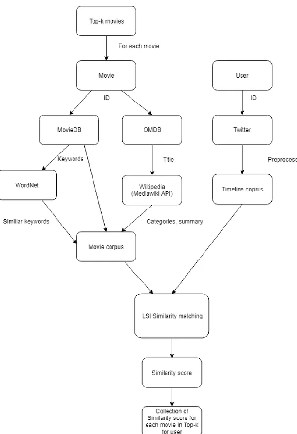
The social media matching module of the recommender system matches all movies in the top-k recommendation list passed on to it with the pre-processed tweets from the user. The dataflow inside the social matching module is shown in Figure 8. The social matching is done by assembling separate corpora of words for both a user’s tweets and for each movie. The corpus of words for each movie is created through a pipeline of different Web APIs. The user tweet corpus is pre-processed as described in section 4.1.1. Each movie corpora is matched with the user’s tweet corpora using LSI and cosine similarity. The list of resulting scores for each movie are sent back to the recommender system and the top-k is rearranged depending on the matching score of each movie.

(41)

31

Figure 8. Social match module diagram depicting the data pipeline and social matching process in the social module.

(42)

32

Movie Corpus

For each movie, a corpus of words that describe the movie is generated. The pipeline for this process consists of OMDB, MovieDb, Wordnet, and MediaWiki. All of them are accessed through rest APIs that return data requested.

In a final step for creating the movie corpus, the collection of words extracted from the different web services need to be pre-processed with the same techniques as user tweets. This is necessary to ensure that the LSI algorithm has the best preconditions for matching similarity in the two corpora.

OMDB

OMDB is a user-generated Movie database Web service (Online movie Database API, n.d.). It can be accessed through a rest API. OMDB can be used to obtain movie metadata like title, year, genre, directors, actors, etc. It accepts the IMDB movie ID, that is found for each movie reviewed in the MovieTweetings dataset, as a query parameter for requests. This is used to convert the IMDB movie ID to a Title and year for each movie.

MovieDB

MovieDB is also a user-generated movie database that can be accessed through a REST API (The Movie database API, n.d.). It is used to request movie keywords. These are a collection of words that describe the movie.

WordNet

WordNet is a lexical database that can be used to get similar words, not only in the sense of word forms and strings of letters but also in the senses of words themselves (Miller, 1995). Through an HTTP API, similar words can be requested for a query. By querying the WordNet API with the keywords for each movie, the keywords are expanded to a bigger collection of words representing the movie.

MediaWiki

MediaWiki is the engine software on which Wikipedia is built on (MediaWiki API, n.d.). The MediaWiki API enables access to the data on Wikipedia through a web service. By querying the API with the Movie title converted from the movie ID through OMDB corpus of words for each movie is further expanded. The data that is added to the corpus of each movie from Wikipedia through MediaWiki API is categories and summary.

Categories are groupings of related pages to the Wikipedia movie article and summary is the summary of each Wikipedia movie article that can be found at the top of a Wikipedia article.

(43)

33

5. Result

In this section, results are presented in the form of general statistics about the system observed after running the dataset and experiments. Each experimental setup is presented in table form. Each table of results is accompanied by a brief description of the experimental setup and its result. Indices showing a result of specific interest are shown in bold.

5.1 General statistics of the systems

The 100 000-ratings dataset used for all experiments except for experimental setup 7 contains 1188 users and 2867 movies. From these 1188 users’ tweets could only be extracted and used from 724 users since the other user’s Twitter accounts were either private or deleted

.

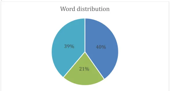
Figure 9 distribution of languages in tweets extracted

A total of 18 769 296 words, numbers, symbols, emoji, and web addresses were found in the tweets extracted from Twitter for the 724 users who did not have a private or deleted Twitter account. From these 18 769 296 only 11 220 676 where Latin character words and only 7 285 873 of these Latin character words were identified as English words through English dictionary lookup.

40%

21% 39%

Improving movie recommendations through social media matching

Examensarbete

15 högskolepoäng, grundnivå

Förbättring av filmrekommendationer

genom social media matchning

Improving movie recommendations

through social media matching

Roman Kuroptev

Anton Lagerlöf

Sammanfattning

Abstract

Glossary

Table of contents

1. Introduction

1.1 Research question

1.1.1 Objective

1.2 The structure of this thesis

2. Background

2.1 Literature review

2.2 Recommender systems

2.2.1 Overview

2.2.2 Content-based filtering

2.2.3 Collaborative filtering

2.2.4 Model-based collaborative filtering using Matrix factorization

2.2.5 Memory-based collaborative filtering using KNN

2.2.6 Twitter as a data source

2.3 LSI

2.3.1 Vector space model

2.3.2 Latent Semantic Index

2.3.3 Cosine similarity

𝑠𝑖𝑚𝑖𝑙𝑎𝑟𝑖𝑡𝑦 = 𝑐𝑜𝑠 (𝛩) =

𝐴 ∗ 𝐵

|𝐴||𝐵|

2.4 Evaluating recommender systems

2.4.1 Item ranking prediction

2.4.1.1 Mean average precision

2.4.1.2 Normalized Cumulative Discounted Gain

𝐼𝑑𝑒𝑎𝑙 𝐷𝐶𝐺

= 𝐼𝐷𝐶𝐺

= ∑

𝑟𝑎𝑡𝑖𝑛𝑔(𝑖)

𝑙𝑜𝑔

(𝑖 + 1)

𝐷

3. Method

3.1 Design creation methodology

3.1.1 Activity 1

3.1.2 Activity 2

3.1.3 Activity 3

3.1.4 Activity 4

3.1.5 Activity 5

3.1.6 Activity 6

3.2 The data

3.2.1 MovieTweetings

3.2.2 Pre-processing the dataset

3.2.3 Sentiment classification

3.2.4 Twitter Data pre-processing

3.3 Experiments & Evaluation

3.3.1 Selected DS evaluation criteria

Criteria 1: Functionality

Criteria 2: Consistency (consistent behavior, stability)

Criteria 3: Accuracy (correctness and preciseness)

Criteria 4: Performance

3.3.2 Experimental overview

3.3.3 Main instance parameters

Purpose and parameter tuning

3.3.4 Two underlying algorithms

3.3.5 Randomization of top-k

3.3.6 Experiments

Experiment 1: Weighted Matrix Factorization (E1)

Experiment 2: Weighted Matrix Factorization with precision at k

threshold (E2)

Experiment 3: KNN(E3)

Experiment 4: KNN with precision at k threshold (E4)

Experiment 5: Optimal user (E5)

Experiment 6: Execution time of Artefact (E6)

Experiment 7: Execution time of offline- versus online-social matching (E7)

3.4

Method discussion

4. Design & implementation