Addition of the direct radiative effect of atmospheric aerosols into the Regional Atmospheric Modeling System (RAMS), The

(1)

000 Center for Geosciences/Atmospheric Research under grant

DAAD19·02·2·0005

THE ADDITION OF THE DIRECT RADIATIVE EFFECT OF

ATMOSPHERIC AEROSOLS INTO THE REGIONAL

ATMOSPHERIC MODELING SYSTEM (RAMS)

by David Stokowski

(2)

THE ADDITION OF THE DIRECT RADIATIVE EFFECT OF ATMOSPHERIC AEROSOLS INTO THE REGIONAL

ATMOSPHERIC MODELING SYSTEM (RAMS)

BY

DAVID M. STOKOWSKI

DEPARTMENT OF ATMOSPHERIC SCIENCE

COLORADO STATE UNIVERSITY

FORT COLLI NS, CO 80523

RESEARCH SUPPORTED BY

DEPARTMENT OF DEFENSE CENTER FOR GEOSCIENCES/ATMOSPHERIC

RESEARCH (CG/AR), UNDER COOPERATIVE AGREEMENT #DAAD-19-02-2-2005

1 NOVEMBER 2005

(3)

ABSTRACT

Forecasting of the radiative impact of atmospheric aerosol species is one of the largest problems remaining in detennining the magnitude of expected climate change over the next century and beyond. While much has been accomplished to achieve this goal, little has been done to this end in regional and mesoscale forecasting models. Models

including the aerosol radiative effect would allow for prediction of small-scale visibility degradation features, as well as more complete investigation of the radiative impact of aerosols on everyday weather.

Inthis project, the direct radiative effect of three atmospheric aerosol species was added to the Regional Atmospheric Modeling System (RAMS). Ammonium sulfate, sea salt and mineral dust were treated in an analogous manner to the hydrometeor species already in RAMS-they are assumed to have a log-nonnal size distribution, and are allowed to advect within. the model. The aerosols are assumed to interact with short- and longwave radiation, using Mie theory as a basis for these interactions. RAMS was set-up using a 2-D LES-type simulation with each model run initialized horizontally homogeneously, using a two second time step, for a total of 78 hours of simulation time. A matrix of

(4)

model runs was completed using assumed concentrations of ammonium sulfate and sea salt, with three experimentally determined mineral dust concentration profiles taken from the SaHAran Dust Experiment (SHADE). The effect of the presence of ammonium sulfate was negligible in nearly every field evaluated, while sea salt showed only minor changes to the downwelling longwave radiation profiles, as well as visibility profiles.

The most dramatic changes to the temperature and radiation profiles in the model were due to the radiative activity of mineral dust. First, where the elevated mineral dust concentrations are present, the atmospheric temperature is increased (up to 3°C per day), as mineral dust has a large imaginary part of the refractive index. The downwelling shortwave radiation is also decreased anywhere from 100-470W/m2through the dusty layers. Unfortunately this value is upwards of four times too great, as the maximum effect during the SHADE campaign was measured by Haywood, et. al(2003)to be-129 ± 5W/m2• Once sensitivity studies looking at the changes in the imaginary part of the

refractive index of mineral dust were completed, the maximum downwelling shortwave forcing from the model was reduced to-141W1m2

• The overall prediction of visibility

was also in the correct sense, but was not able to be quantitatively tested.

The initial results from this study are qualitatively positive. Once both three-dimensional testing is completed, and more accurate values of the refractive index of aerosol species are available (especially for mineral dust), the quantitative results can be used to check on

(5)

specific cases of visibility degradation, as well as how the radiative impact of aerosols will affect everyday weather phenomena.

David M. Stokowski Department of Atmospheric Science Colorado State University Fort Collins, CO 80523 Fall 2005

(6)

ACKNOWLEDGEMENTS

I would first like to acknowledge and thank Dr. William Cotton for taking a chance on me as a graduate student, as well as for his continued guidance and insight during the preparation of this paper. Also deserving thanks are Dr. Christian Kummerow and Dr. David Krueger for their time and thoughtful consideration of this work. As Dr. Cotton's research group has been of invaluable help, I would like to thank group members both past and present for imparting their knowledge upon me: Jerry Harrington, for his utmost patience in helping a new user understand the beast that it RAMS; Dr. Graham Feingold whose Mie scattering code forms the foundation of the radiation subroutine added to RAMS: to Dr. Hongli Jiang and Dr. Gustavo Carrio for their assistance in using RAMS as an LES-model; Dr. Susan van den Heever as a guide and giver of sage advice to a master's student; to Steve Saleeby as a constant help and source of scientific discussion, to Liz Zarovy for her help in understanding current avenues of aerosol research, both scientifically and as it relates to RAMS; to R. Todd Gamber and Jeremy Orban for robbing me of the joy of driving to and from Fort Collins, by keeping the RAMS computer network up, and accessible from my home; and to Brenda Thompson whose help saved me countless hours of work, and whose conversations gave me perspective impossible to have gained on my own. I wish to give my deepest gratitude to Jim

Haywood of the

u.K.

Meteorological Office, without whose guidance, patience, help and unlimited access to SHADE data, this project would not have been possible. To Luke

(7)

van Roekel, constant friend, intellectual stimulator, technical editor, source of comedy, and keeper of the futon - your friendship and support will mean more to me than you will ever know. To my dearest wife, best-friend and mother our child-Rachel, you are a saint for continuing to support me in these seemingly endless and unconnected

endeavors; your love and faith in me brings me to tears. To Benjamin, your innocence and presence have shown me what is truly important. And finally, to my Lord, Jesus Christ; after all of this 1 now truly understand what Paul wrote in Philippians 4: 13 - "I can do all things through Him who strengthens me."

This study was graciously and generously supported by the Department of Defense Center for Geosciences/Atmospheric Research, under cooperative agreement #DAAD 19-02-2-0005.

(8)

CHAPTER 5 - SENSITIVITY STUDIES...

60

5.1 - Model Sensitivity to Initial Sea Salt Concentrations... 60

5.1.1 - Changes in the Temperature and Moisture Profiles. 60 5.1.2 - Changesinthe Radiation Streams... 62

5.1.4 - Investigation into Visibility... 63

5.2 - Model Sensitivity to Changes in Refractive Index... 63

5.2.1 - Changes in the Temperature and Moisture Profiles... 64

5.2.4 - Investigation into Visibility.. 67

5.3 - Discussion of Results... 68

CHAPTER 6 - CONCLUSIONS...

70

6.1 - Summary and Conclusions... 70

6.1.1- Summary of Work... 70

6.1.2 - Conclusions... 72

6.1.3 - Scientific Implications of the Work... 74

6.2 - Recommendations for Future Work... 75

(10)

CHAPTER

1 -

INTRODUCTION

1.1 INTRODUCTION TO AEROSOLS

The American Heritage Dictionary defines an aerosol as "a gaseous suspension of fine solid or liquid particles." Meteorologically speaking, an aerosol is commonly defined as only the particulate matter (Seinfeld and Pandis, 1998). There are many types of aerosols that are prevalent in today's atmosphere: ammonium sulfate, sea salt, mineral dust, black carbon from industrial processes, smoke, and the list goes on. Aerosols can be classified in two different manners: they can be divided by causation as either natural or

anthropogenic; or by formation as either primary (lofted from the surface) or as

secondary (formed in the atmosphere). Mineral dust aerosols are primary aerosols whose mobilization is sensitive to factors including soil moisture and surface wind velocities (Ginoux, et. aI, 2001). These mineral dust sources can be both natural, as from deserts, or anthropogenic as from desertification through land-use changes (Myhre and Stordal, 2001; Tegen, et. aI, 1996). Similarly, sea salt production is also a function of surface wind speed through formation and subsequent evaporation of "film-" and "jet droplets" (Prupppacher and Klett, 1978). Black carbon has a variety of sources, the most prevalent of which are from biomass burning, and residential fuel burning (Streets, et. aI, 2004). In urban areas, emissions from diesel trucks also contribute greatly to the global black carbon burden (Schauer, et. aI, 1996). Atmospheric sulfur aerosols (commonly referred

(11)

to as sulfates) also have both natural and anthropogenic sources. Anthropogenic sulfates are emitted through industrial processes and fossil fuel burning, and account for

approximately 65% of the global sulfate burden (Chin and Jacob, 1996 and Chin, et. aI, 2000). Most natural sulfur is emitted as dimethylsulfide (DMS) from phytoplankton, and accounts for the remaining 35% of the global sulfate burden (Chin and Jacob, 1996; Chin, et. aI, 2000). Each of these aerosols has some effect on the atmospheric radiation

balance, but very few numerical weather prediction models take this effect into account, due to poor knowledge of spatial and temporal sources and sinks of the individual aerosols (Andrews, et. aI, 2004; Sokolik and Toon, 1996).

1.2 IMPORTANCE IN FORECASTING AEROSOLS

In recent years, the United States Military has increased its worldwide presence in areas susceptible to rapid changes in visibility due to airborne mineral aerosols. This issue was first documented during Operation Desert Storm in Iraq beginning in 1990, and has continued during Operation Enduring Freedom in both Iraq and Afghanistan since 2001. Kuciauskas, et. al (2003) recognized many of the problems that occurred in Iraq during frequent dust storms in the spring of 2003. From an operational cost standpoint, dust storms can degrade the performance of ground-based vehicles, which therefore require more frequent clean up and maintenance. As dust inhibits visibility, operations using laser-guided munitions are greatly limited. Soldiers "getting lost" in dust storms was also cause for great concern. Minimizing the loss of human-life is paramount in conducting operations in dust storm conditions. The most recent example for the need to accurately forecast dust came in the April 16, 2005 crash of a military helicopter in Afghanistan. It

(12)

was reported that low visibility caused by a dust storm was present at the time of the crash, killing 16 people during activities carried out as a part of Operation Enduring Freedom.

The importance of forecasting aerosols is also manifested in the civilian realm. One of the main points in the Executive Summary for Policy Makers of the International Panel on Climate Change's (IPCC) Third Assessment Report is that "[e]missions of greenhouse gases and aerosols due to human activities continue to alter the atmosphere in ways that are expected to affect the climate" (lPCC,2001). While our understanding of the future climate effects due to the so-called greenhouse gases is high, there is a low level of scientific understanding related to aerosol effects on future climate (IPCC, 2001). In fact IPCC states that the magnitude of the direct aerosol forcing could be on the same order of magnitude as that of the greenhouse gases, but in a negative sense (lPCC, 2001). The presence of aerosols can increase the effective albedo of the planet, through processes such as the Twomey (1977) Effect, where anthropogenic sulfate aerosols would increase the number of cloud droplets for a given water vapor content, causing a greater number of small droplets and hence a more reflective cloud. However, much of the trouble in determining the direct radiative effect of aerosols is that there is a very limited data set containing information about the spatial and temporal gradients ofatmosph~ricaerosols (Andrews, et. aI, 2004; Sokolik and Toon, 1996). Despite this, it is thought that

ammonium sulfate has an overall cooling effect on Earth (Ramanathan, et. aI2001). Depending on the size and location of mineral dust aerosol particles, they can have either a heating or cooling effect (Sokolik and Toon, 1996), while the anthropogenic forcing of mineral aerosols has been shown to have a cooling contribution (Tegen, et. ai, 1996).

(13)

Black carbon aerosols most often show a warming contribution to atmospheric forcing (Streets, et. aI, 2004; Conant, et. aI, 2002). Unfortunately, a literature search yielded no useful published information about the effect of sea salt particles on atmospheric temperature changes.

While many of the more widely known aerosol effects are given in terms of global-scale interactions, any modification to radiation streams within a numerical weather prediction model will have effects on model outputs. A recent modeling study of the presence of a Saharan Dust layer during the Cirrus Regional Study of Tropical Anvils and Cirrus Layers - Florida Area Cirrus Experiment (CRYSTAL-FACE), caused a decrease in modeled total precipitation over a control run with only background concentrations of mineral dust (van den Reever, et. aI, 2005). On an ever smaller scale, Miller, et. al (2004) discuss that the presence of a layer of dust will decrease turbulence in the planetary boundary layer, due to decreased down-welling solar radiation, and hence decreased turbulent flux of sensible heat into the boundary layer. This also leads to a decrease in surface winds, through a decrease in downward transport of momentum, and hence a decrease in the amount of dust that can be lofted into the atmosphere (Miller, et. aI, 2004). Therefore, in order to increase the accuracy of numerical weather prediction models on any scale, the inclusion of the radiative effects of aerosols is a desirable means toward that end.

(14)

1.3 HISTORY OF NUMERICAL MODELING WITH AEROSOLS

Over the past fifteen years, a number of numerical weather prediction models have been modified to allow for prediction on aerosol concentrations as well as their effect on the radiation streams within the parent code. Erickson, et. al (1991) introduced a 3-dimensional global sulfur cycle model to include sulfate aerosol effects on cloud nuclei (CN) concentrations. Their research was able to confirm a strong positive relationship between CN concentrations and sulfate. A few years later, Boucher, et. al (1995) specifically investigated the direct radiative effect due to the sulfur cycle, in a general circulation model (GCM) framework. The testing showed a relatively low sensitivity of changes in energy fluxes to sulfate aerosol size and composition, leading the authors to believe that sulfate concentration may be the only variable necessary to determine a good estimate of the sulfate radiative forcing (Boucher, et. aI, 1995).

The initial foray into 3-dimensional modeling containing dust was performed by Joussaume (1990). This global climate model was able to simulate many seasonal dust plumes qualitatively well, while recognizing that many oversimplified parameterizations were used (e.g., dust mobilization from wind speeds). The mineral dust model of Tegen and Fung (1994) became the first to account for dust particle size in radiative forcing calculations, while parameterizing sources and sinks of dust.

In the past few years, modeling with aerosols has become more commonplace, and the scale at which these models are being run is also decreasing. As a recent example, the Georgia Tech/Goddard Global Ozone Chemistry Aerosol Radiation and Transport

(15)

(GOCART) model has simulated the sulfur cycle, mineral dust cycle and carbon cycle (e.g., Chin, et. aI, 2000; Chin, et. a12002; Yu, et. aI, 2004), to yield their radiative forcing on the global scale. The estimated global annually averaged change in surface radiative forcing is -9.9W/m2_{for all atmospheric constituents (Yu, et. aI, 2004). On a smaller}

scale, Qian, et. aI, (2003) ran a regional climate model over China and was able to reproduce cooling that has been taking place in China over recent decades. The crux of their paper was that the cooling (up to -14W/m2_{or -1.2°C) was present when their model}

accounted for the direct radiative effect of ammonium sulfate, methane sulfonic acid, organic carbon, black carbon, sea salt and soil dust.

1.4 OBJECTIVE OF THIS RESEARCH

The main scientific objective of this research was to modify the Regional Atmospheric Modeling System at Colorado State University (hereafter RAMS) to account for the direct (and semi-direct) effect of atmospheric aerosols. A new module containing the FORTRAN code was created and integrated into the existing RAMS framework. The novelty of this approach is that all previous works on the addition of the direct radiative effect of aerosols to a numerical weather prediction framework were under global or regional climate model frameworks, whereas RAMS specific design is to be a mesoscale forecasting model. This new module updates the bulk optical properties of optical depth (t), single scatter albedo (w) and the asymmetry parameter (g), by combining the aerosol optical properties (aerosol direct effect) with cloud droplet and hydrometeor optical properties. These updated values are fed back into the model, modifying the atmospheric column heating rates and hence influencing the microphysics, constituting the semi-direct

(16)

effect. Because the aerosol direct effect is now accounted for, a simple code modification was made to determine a visual range, and hence a new forecast variable has become available. The new code has been tested using real data collected during the SaHAran Dust Experiment (SHADE) campaign, which was conducted over the Cape Verde Islands and other areas to the west of continental Africa. Atmospheric temperature and moisture profiles, values of radiation extinction along with radiation fluxes from RAMS have been compared to measurements made using a C-130 aircraft during SHADE.

The remainder of the paper will be organized in the following manner. A discussion about the history and governing equations of RAMS can be found in chapter 2. Chapter 2 also contains a discussion about the modifications made to RAMS, with details about the use and applicability of Mie scattering theory of radiation as well as the off-line code, which was used to generate the optical property look-up tables employed within RAMS. The goals and specific data used in the validation study from the SHADE campaign are presented in chapter 3. Chapter 4 contains information about the model-testing phase, including detailed set-up information as well as model results. Two simple sensitivity studies on the model results to the initial concentration of sea salt and the assumed absorptivity of mineral dust are the foci of chapter 5. A summary of the work with all pertinent conclusions, along with suggestions for future work can be found in chapter 6.

(17)

CHAPTER

2 -THE MODEL

2.1 THE REGIONAL ATMOSPHERIC MODELING SYSTEM (4.3.0)

The Regional Atmospheric Modeling System (RAMS), which was developed at Colorado State University, made its debut under the current architecture in 1991. This work was the merger of three previous mesoscale models: a non-hydrostatic cloud/mesoscale model (Tripoli and Cotton, 1982), a hydrostatic version of the above cloud/mesoscale model (Trembeck 1990) and a mesoscale sea-breeze model (Mahrer and Pielke, 1977). Since its 1991 debut, many updates to RAMS have been made, most of which are documented by Cotton et. aI, (2003).

For this study, RAMS version 4.3.0 was used. Large sections of RAMS code will not be discussed, as they were not specifically needed in the development and testing of the new radiation module. RAMS uses non-hydrostatic and Reynolds-averaged momentum and mass continuity equations as described in Tripoli and Cotton (1986). A leap-frog time differencing scheme is used to calculate pressures via the Exner function, with a forward time-differencing scheme used for all other prognosed variables. There are a total of 12 prognosed variables within RAMS: the u,v andw wind components, the ice/liquid water

equivalent potential temperature (eil),thedryair density, total water mixing ratio, and

(18)

aggregates). From these variables, pressure, potential temperature, vapor mixing ratio, and cloud mixing ratios (small and large cloud droplet modes) can all be diagnosed.

The RAMS model uses a C grid setup (Arakawa and Lamb, 1981; Randall 1994), allowing for straightforward calculation of the individual components of the vorticity equation. The user can define the grid to be either a Cartesian grid, or a polar

stereographic grid. The terrain-following vertical coordinate,Ozis used in RAMS

(Gal-Chen and Somerville, 1975; Clark, 1977). RAMS also has the capability of employing two-way interactive nested grids, where the nested grid contains higher horizontal resolution than its parent. These nested grids may (but are not required to) have enhanced vertical resolution.

The microphysics subroutines in RAMS were first developed and described by Verlinde, et. al (1990). This work showed that analytic solutions to the collection equations were possible if one assumed that the collection efficiencies were constant, allowing for prediction on the mixing ratio and concentrations of any of the hydrometeor categories within RAMS. Walko et. al (1995) describes how this was implemented within the RAMS framework. Later, Meyers et. al (1997) extended this prediction to mixing ratio and number concentrations of each of the hydrometeor species. Most recently, a second cloud droplet mode has been added to RAMS to better represent the dual mode of cloud droplets most often observed in nature (Saleeby and Cotton, 2004). For turbulence parameterizations, RAMS has a variety of user specified turbulence closure schemes to choose from, including the Smargorinsky (1963) deformation-K closure scheme, the

(19)

Mellor-Yamada (1982) ensemble-averaged TKE scheme and the Deardorff (1980) scheme, where eddy viscosity is a function of TKE.

Harrington (1997) developed the current radiation subroutines that were modified in this study. The radiation code uses a two-stream structure, computing the upwelling and downwelling components by integrating the azimuthally independent radiative transfer equation and applying the 6-Eddington approximation to solve this equation numerically (Harrington, 1997). These radiation calculations are done on eight broad radiation bands, three in the solar region and five in the near infrared. This eight-band structure was chosen to mimic the treatment of gaseous absorption and Rayleigh scattering of water vapor, carbon dioxide, and ozone of Ritter and Geleyn (1992). The overall scattering of radiation within RAMS also accounts for scattering due to the presence of the eight previously mentioned hydrometeor categories (Harrington, 1997). In order to allow these particles to interact with the radiation, three variables need to be defined: the optical depth (t), the single scatter albedo (00) and the asymmetry parameter (g). The optical depth is a proxy for total extinguished radiation, where the single scatter albedo describes what fraction of the extinguished radiation is scattered (absorption is the other assumed extinguishing process), and the asymmetry parameter describes the direction in which radiation is scattered as the intensity weighted average of the cosine of scattering angle (Seinfeld and Pandis, 1998). This information is then used to update the atmospheric heating rate profiles, and hence thermal properties throughout the modeL

(20)

2.2 MODIFICATION TO RAMS

The main scientific objective of this research was to add the direct and semi-direct radiative effects of aerosols into RAMS. Itwas determined that the best way to treat the particles was to assume that they were smooth spherical scatterers and absorbers, so that Mie scattering theory could be applied. Therefore the only required input information is the refractive index of given aerosol particles as a function of the wavelength of the incident radiation, as well as the particle size (usually as a radius) and the wavelength of the radiation involved in the interaction. This allows for direct calculation of the total amount and direction of the extinguished and scattered radiation. Once this aerosol effect was accounted for, it was combined with the optical depth('t), the single scatter albedo

(w) and the asymmetry parameter (g) from the cloud hydrometeors, giving a new total't,

wand g. The remainder of this chapter describes the details of the new module containing the aerosol direct effect.

2.2.1 BACKGROUND ON MIE THEORY

The interaction of radiation with particles is a problem that has no general analytic solution. However, with a few assumptions about the nature of the radiation-particle interaction, exact solutions can be derived. If there is no change in the wavelength of the radiation interacting with a particle, (otherwise known as elastic scattering), and if the particles causing the radiation to scatter are spherical, then the exact solution can be found using Mie (1908) theory. The elasticity assumption basically means that a photon can either change directions, or be absorbed as a change in internal energy. Since

(21)

bonding on the atomic level is beyond the scope of this study, it is reasonable to assume that changes in internal energy of a molecule are manifested solely through temperature changes. There is, however, a small body of research describing the validity of the spherical particle assumption as it relates to mineral aerosols. Pollack and Cuzzi (1980) explain that a mixture of small irregularly shaped particles, are expected to exhibit similar scattering behavior to an equivalent volume of spheres. This breaks down for elongated particles with a large total refractive index (Pollack and Cuzzi, 1980). However,

Mishchenko et. al (1997) found in a theoretical study, that the optical depth, single scatter albedo and the asymmetry parameter are only slightly different when spherical and non-spherical particles are compared using a known optical depth (i.e., known concentration).

Ittherefore seems plausible to assume that our use of Mie Theory for this application is entirely reasonable.

In order to use Mie theory properly, three key parameters are needed: the wavelength of the incident radiation, the size of particle, and the total complex refractive index (Seinfeld and Pandis, 1998). The first two of these parameters are often used together to create a dimensionless size parameter (radius of particle divided by wavelength of radiation). The complex refractive index insures that wavelength dependent information about the

absorption and scattering of the particle is taken into account. Once all of this information is sent to a "canned" Mie scattering routine, values for't, wand g can be easily obtained.

(22)

2.2.2 THE MIE SUBROUTINES

Inorder to get optical property values necessary for the RAMS radiation subroutine, a method to calculate these values using Mie theory was needed. The "canned" Mie scattering routine used in this study, called equim_5, was developed by Graham Feingold of the National Oceanographic and Atmospheric Administration (NOAA), [personal communication]. For the equim_5 code, only one input variable is needed, the complex refractive index of each aerosol species, all other necessary variables are internally defined. The refractive indices used in this study were adapted from d' Almeida, et. al (1991).

The equim_5 code was used to model three different aerosol species: ammonium sulfate, sea salt and mineral dust. One of the most convenient features of the equim_5 code allows the aerosol species to be either uniform, or an internal mixture, specifically a shell/core mixture. Ammonium sulfate was the only of the three species to be modeled with an insoluble core-having 10% (by mass) ammonium sulfate on a 90% insoluble core of mineral dust. Sea salt was assumed to have no insoluble core, while mineral dust had no soluble outer coating. The equim_5 code was run for each of these three aerosol species, generating 4 tables each: one containing the extinction coefficient (qext)' one containing the scattering coefficient (qscat)' one containing the asymmetry parameter (gasym) and one containing a deliquescence growth factor. The three optical property tables are a function of radiation band, particle size and relative humidity, whereas the deliquescence growth factor table is a function of particle size and relative humidity only.

(23)

Again, the only required input to the equim_5 code is the complex refractive index of each aerosol species as a function of wavelength. The particle size, and wavelength of radiation needed for Mie theory calculations are internally defined within the equim_5 code. Initially, the code defines a lower particle size limit at 15nm. From there, bin limits are created by determining the radius of particles for a mass four times greater than the mass at the previous bin limit. In order to best represent the larger particles in the model, seventeen bins were chosen, so that the largest bin limit is at 3.048 microns. Each bin is assigned a representative radius by taking the average of the lower and upper masses for each bin, as determined by the bin limit radii. Next, the radiation bands were chosen to mimic the eight bands currently in RAMS--three in the solar spectrum and five in the near-infrared. Each of the eight radiation bands was split into 100 smaller bands, each with an average wavelength. Now, since specific wavelengths of radiation and particles sizes were chosen, the Mie solution can be exactly calculated. At each small wavelength band, the model determined the intensity of the resultant scattered radiation in 10

increments, to determine the extinction coefficient, the scattering coefficient and the asymmetry parameter. The value determined for each broad radiation band was a simple arithmetic mean of the values for the 100 smaller radiation bands. Finally, the

deliquescence effect was determined by setting up relative humidity boundaries from 80% to 99%, in 1% increments. No deliquescence growth is assumed for environmental relative humidities of 80% or lower. The end result of this code is the four output tables as described above. Because the Mie theory solution to this problem is exact, it only needs to be computed once. Therefore, the results of this subroutine are placed in a

(24)

look-up table within RAMS, to increase the speed at which the model can calculate the overall changes in 't, 00 and g.

2.2.3 THE "OLD" RADCALC3 SUBROUTINE

Harrington (1997) wrote the

on driver ation driver From radiati

"

Initialize atmospheric soundings

•

Determine cloud optical properties

•

Determine shortwave radiative fluxes

•

Determine longwave radiative fluxes Back to radi ,r thickness ('t), the single

asymmetry parameter (g), due scatter albedo (00) and the determines the optical Figure 2.1). The code first subroutine radcalc3 (see

property values for optical The meat of this code lies in radiation code for RAMS. current version of the

to cloud droplets and Figure 2.1: Flow chart of the original radiation scheme by Harrington (1997).

hydrometeors. Next, path

lengths for water vapor, carbon dioxide and ozone (gases active in the Rayleigh scattering regime) are computed. Once this is complete, the code determines the downward solar fluxes and the Rayleigh scattering of this radiation caused by water vapor, carbon dioxide and ozone. Next, the blackbody fluxes are calculated over the five infrared bands, to give the two-stream results for all eight radiation bands. The three solar bands and the five infrared bands are treated separately, so that both longwave and shortwave heating rates

(25)

can be separately determined. This information is then passeq back into the model for modification of the ice-liquid potential temperature,Sil'

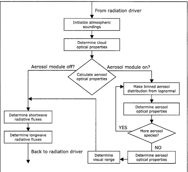
2.2.4 THE NEW AERORAD SUBROUTINE

Before discussing the new code, it is important to understand how aerosols are represented with in RAMS. As discussed previously, the aerosols are treated using a shell-core model. The remainder of the parameters describing aerosols are treated in an analogous manner to those describing hydrometeors. The number concentration of each aerosol species is assumed to be distributed log-normally, with a shape parameter of the distribution set at 1.8. The aerosols are also allowed to advect throughout the model. Finally, a number concentration and median radius of the distribution are both predicted for each aerosol species at each grid point. When the aerosol portion of the radiation subroutine is accessed (see Figure 2.2), through the radcalc3 subroutine, each aerosol category is treated separately, and these calculations are performed at each grid point. First, the total number concentration and median radius values are fed into a routine that creates a binned distribution of the aerosol. A look up table approach is used, where the percentage of the total concentration in each of the 17 bins was determined for 26 different median radii. A third order Lagrangian interpolation was used to determine the bin concentration for the given median radius. The binned concentrations were then fed into a subroutine that determines the total extinction and scattering, using the previously described look-up tables containing qexl' qscat, gasym and the deliquescence growth factor. The amount of extinguished radiation, scattered radiation and forward-scattered radiation were determined based on binned aerosol concentrations of the aerosol in question and

(26)

From radiation driver

Initialize atmospheric soundings

Determine cloud optical properties

Aerosol module off? Aerosol module on?

Make binned aerosol distribution from lognormal

Back to radiation driver

Determine visual range

Determine aerosol optical properties

Figure 2.2: Flowchart of the new aerosol radiation scheme.

the relative humidity the aerosol were subject to. This process is then repeated until all active aerosols have been accounted for at which point the extinction and scattering values were summed together at each grid point. The summed values for the total extinction, total scattering and forward scattering were then added to their analog from the cloud droplets and hydrometeors. Slingo and Schrecker (1982) developed the method for determining the optical depth (t), the single scatter albedo (OJ) and the asymmetry parameter (g), from the values of scattering and extinction calculated from the aerosol subroutines, which are already weighted by a model-layer thickness:

(27)

g

=

total forward scattering/total scattering 00

=

total scattering/total extinction

't

=

total extinction

These values of't, 00 and g now contain information about the direct aerosol effect in the model, and are sent onward to the remainder of the radiation scheme.

Once the optical properties were combined to yield an overall value of the optical depth ('t), the single scatter albedo (00) and the asymmetry parameter (g), a simple equation was used to determine visual range. The Koschmieder equation is simply:

Xv

=

3.912

*

bex! / (dzl

*

1000)

Where, bex/dzl is the optical thickness of the radiation band containing the visible spectrum,Xvis the visual range and both bex!andXvhave the same length units (i.e.,

meters, kilometers, etc.). This equation was empirically determined, assuming that an "average" human eye can distinguish a contrast value of 2% (Seinfeld and Pandis, 1998). The visual range is a scalar value that is determined for each grid cell, and is not pathway dependent.

(28)

CHAPTER

3 -THE SAHARAN DUST

EXPERIMENT

3.1 BACKGROUND ON THE SAHARAN DUST EXPERIMENT

The impact of atmospheric aerosols, as it relates to climate change, is still one of the most uncertain variables (International Panel on Climate Change, (IPCC), 2001). Dust

aerosols are of particular importance, due not only to their scattering and absorption of solar radiation, but the perturbation they introduce in the terrestrial radiation spectrum (Tame, et. aI, 2003). The Saharan Dust Experiment (SHADE) was designed to

experimentally determine parameters necessary to model the direct radiative forcing of Saharan dust. (Tame, et. aI, 2003) This was achieved by collecting concurrent

measurements of radiances and irradiances together with physical and optical properties of atmospheric aerosols, in order to provide a radiative closure between in situ and remotely sensed data. The experiment was conducted under the auspices of the UK Meteorological Office, taking place between 19 and 29 September 2000 off the coast of Mauritania in and around the Cape Verde Islands.

3.2 SYNOPTIC WEATHER CONDITIONS DURING SHADE

The specific data used from the SHADE campaign for this study, was collected on the 24th_{and 25}th _{of September 2000. These profiles were chosen due to the presence of the}

(29)

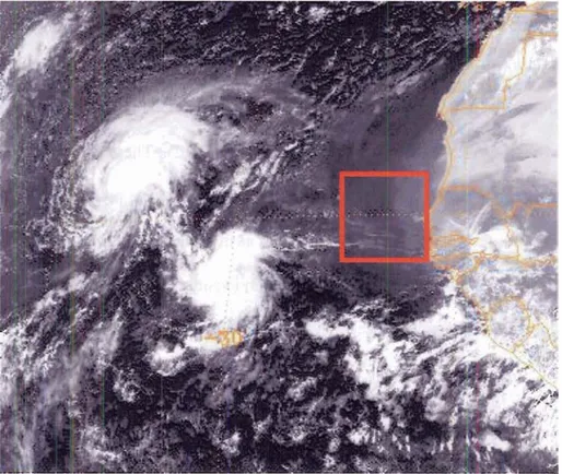
Saharan dust layers, and that the structure of these profiles was each markedly different, in terms of the vertical distribution of dust concentrations. Both days were relatively cloud-free in the area of sampling, despite slight discolorations present in the

METEOSAT satellite field (See figures 3.1 and 3.2). These discolorations are due to the presence of dust. There was no widespread airborne dust present on the 24th

,but there

were some small scale areas of dust, not easily seen on satellite (see figure 3.1). However, widespread dust was present and visible via satellite images on the 25th(see figure 3.2). Hurricane Isaac is located to the west of the sampling area, and had no

Figure 3.1: METEOSAT image off the western coast of Africa at113OUTC, on 24 September 20aO-red box is approximate location of sampling area.

(30)

Figure3.2: METEOSAT image off the western coast of Africa at 1130UTC, on 25 September 2000-red box is approximate location of sampling area.

impact on the sampling during these two days. The synoptic conditions were relatively benign near the sampling region (in the region of 15°N and 200

W) with little forcing present (see figures 3.3 and 3.4). However, a low-pressure circulation is present over the Sahara on the 24th_{generating surface winds, which were most likely responsible for}

lofting large amounts of dust into the atmosphere. The dust plume generated from this system was over the sampling area on the 25th•

(31)

27 1'18 ,·28136

?

~.Qp 2S~YL21io501 ZDL~2+0%·~

-35 - ~~'OB 2'-25 '-2~ 110603 10 -5 (

Figure 3.3: Surface pressure map, with plotted METARs over western Africa and the eastern Atlantic for 1200UTC on 24 September 2000. 28 221 . ....00+~I .. C6KD92102010,1 27 1'10.4101 102'1· 28 175 ~KR62~~O/ 211 07070" '.;";' . 26 13 :PCD~+20~ 2~...7.t.l~O:\. 30 127 ... .. 3'0 '" u'~~ri~5' -35 OA~F2ol... , -:'>5 -20 10 ··5

Figure 3.4: Surface pressure map, with METARs over western Africa and the eastern Atlantic for 12000UTC on 25 September 2000.

(32)

3.3 RELEVANT INSTRUMENTATION

All of the data used in this report, came from instrumentation aboard the UK Met Office's C-130 aircraft, described in Tame, et. a12003. Location of the aircraft was determined by a GPS transponder, while the meteorological conditions outside the aircraft were measured using a pressure probe, two temperature probes and two dew point/relative humidity probes. The size distribution of the aerosols was determined using a Passive Cavity Aerosol Spectrometer Probe lOOX, (PCASP). Dropsondes were launched periodically throughout the flights of C-130, recording temperatures, dew points, and positional data using GPS transponders. These sondes were launched so that vertical moisture and temperature profiles could be obtained through different Saharan dust layers present during the SHADE campaign. A TSI 3563 nephelometer was used to determine aerosol scattering at three distinct wavelengths in the visible spectrum at 450nm, 550nm, and 700nm. Also on board the C-130 were two broadband radiometers, one facing upward measuring radiation in a band from 0.3 to 3.0!-tm, and one facing downward, measuring radiation from 0.7 to 3.0!-tm.

3.3.1 DUST CONCENTRATION MEASUREMENTS

Throughout the SHADE campaign, the C-130 aircraft was operated on four different days dedicated to collecting data. The two specific days used for this study are the 24th and 25thof September, noted to have moderate and heavy dust loadings respectively. Each day's flight pattern consisted of three main types of legs: straight runs, low altitude orbits and profiles. For this study, three specific profiles were used, the first profile of the day

(33)

on the 24th, and two afternoon profiles on the 25th• All of the dust concentration data was

collected using a Passive Cavity Aerosol Spectrometer Probe (PCASP).

During the entire campaign, the PCASP recorded the aerosol concentrations of 15 different bins ranging from 0.05!-tm to 1.5!-tm, at a time resolution of one second

(Haywood, et. aI, 2003). All of the aerosols counted using the PCASP were assumed to be mineral dust. For this study, the dust concentration data was averaged in lO-second groupings, as was the latitude, longitude and height data. Only the nine largest size bins were used to determine the aerosol concentration (from 0.15!-tm to 1.5!-tm), as the

concentrations in the smaller bin were too noisy. After examining the PCASP data, the dust size distribution was assumed to be the sum of five lognormal distributions

(Haywood, et. al, 2003). In order to be consistent with other ongoing avenues of RAMS research, the dust concentrations have only two modes. Since there is a mismatch in the number of assumed lognormal modes of the dust concentrations, a method was developed to match the five-mode information from Haywood, et. al (2003) to a two-mode

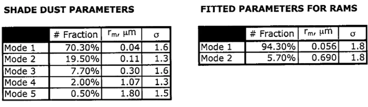
SHADE DUST PARAMETERS FITTED PARAMETERS FOR RAMS

# Fraction rmt !!m _a _# _Fraction

r

mt Ilm a Mode 1 70.30% 0.04 1.6 94.30% 0.056 1.8 Mode 2 19.50% 0.11 1.3 5.70% 0.690 1.8 Mode 3 7.70% 0.30 1.6 Mode 4 2.00% 1.07 1.3 Mode 5 0.50% 1.80 1.5

Table 3.1: Parameters for five-mode dust representation of Haywood, et. al (2003), along with the best fit parameters determined for RAMS.

(34)

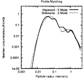
representation to be used in this study (see table 3.1). The parameters for the two-mode representation were determined by minimizing an error cost function

Cost function=~«[five-mode]- [two-mode])2

*

rbin2)

The error cost function is a function of the relative sizes of the two peaks, as well as their median radii. For each cost function, bins were set up from 0.5nm to 4!-tm, with a bin-width of 0.5nm. At each bin, the

Prol1le Malchmg

square of the difference in concentrations of the estimated five-mode dust distribution and the assumed two-mode

distribution, were multiplied by the radius squared-since particle extinction is a strong function of cross-sectional area. The sum

Hayw':lcd • 5 Mode -Stokowski . 2 Mode ••••••

w

.~ 0.1 ~. c: .2 '§ c·.Q1 'E

..

i! (;> 'J _0.001

!

i

0.0001 1e·05 0.001 0.Q1 01

ParlJcle radius~micrQns)

Figure 3.5: Size distributions for the five-mode dust profiles from Haywood, et. al (2003) and from this study. of these errors from 0.5nm to 4um constituted the total cost function. The minimization of the cost function yielded a two-mode distribution as pictured in Figure 3.5, with the five-mode distribution picture for reference. Once the two-mode distribution was determined, the sum of the concentrations of the nine bins from the PCASP were then extrapolated to the entire size domain, to determine an overall concentration value to be used in the model.

There were three dust profiles (see figure 3.6) that were used in this study, one from the initial ascent of the C-130 on 24 September 2000 (profile 1), and two afternoon profiles

(35)

on 25 September 2000 (profiles 2 and 3). Each of these profiles exhibits different magnitudes and locations of the dust concentration maxima. Profile 1, shows a maximum around the level of the marine boundary layer top (800m), with elevated concentrations(300-600/cm3) in the 3000-4800m range. The second profile shows a

small maximum around 1800m, and a much

MirHlral Dust Pro/des 5C<l0 4000 E ~3OO0 €, ~200C' 1000 Low _._ . Medium -High

---more highly concentrated dust(-1200/cm3) in the

2500-4500m layer. Profile 3 shows a strong maximum(-3800/cm3) just above marine

boundary layer top (800-1600m), and again

O -...' - - - - ' - - - - " - - - ' - - . . . . J

o 1000 2000 3000 4QOO 5000 Ccncenlration (in ,\'lcm3)

Figure 3.6: The three dust concentration profiles used in this study.

contains elevated concentrations above 3000m

(600-1200/cm3). Each of these profiles is

markedly different, and according to Haywood, et. al (2003), the height location of each maxima indicates a different source region within the Sahara, as determined by back trajectory analysis.

3.3.2 DROPSONDE MEASUREMENTS

Throughout the measurement campaign, dropsondes were launched to record temperature, moisture and wind profiles at various locations. For this study, the dropsonde most closely located in time and space to the given dust profile was used in comparison to the model results (Table 3.2). All three profiles showed good temporal co-locations (within 25 minutes of the end of a given vertical profile), but the spatial co-locations varied greatly. For the first profile, there was very good spatial co-location,

(36)

while the second profile had moderately good co-location. Unfortunately, there was not a particularly good spatial co-location for the third profile.

Profile # Date Time (UTe) Location (Avg) DroDsonde Point

1 9/24 1012-1037 16.78~N, 22.75~W 16.83 N, 22.49~W, 1050UTC 2 9/25 1501-1518 16.02"N,21.02 W 15.67"N, 20.04

"w,

1535UTC 3 9/25 1729-1745 15.11~N, 18.46"W 15.85°N, 20.45°W, 1810UTC

Table 3.2: Average spatial and temporal locations of the three dust profiles, along with the closest

corresponding dropsonde.

3.3.3 RADIATION MEASUREMENTS

Many different types of radiation measurements were taken during the SHADE campaign. For irradiance measurements in the shortwave, a total of four Eppley broadband radiometers were placed on the C-130 aircraft. Both the upward and

downward facing setups contained one radiometer measuring the 0.3-3.0!!m broadband with a clear dome, and one measuring the 0.7-3.0!!m broadband with a red dome (Haywood, et. aI, 2003). The longwave irradiance measurements were collected using upward and downward facing pyrgeometers covering a broadband of radiation from 3-50!!m (Highwood, et. aI, 2003). Data from theTSI3563 nephelometer recorded the amount of radiation scattered at 450nm, 500nm and 700nm (Haywood, et. aI, 2003). Since the most intense radiation incident on the Earth is near 550nm, that specific channel will be used for comparison to modeled values of extinction and hence will be a check on the modeled visual range. Finally, the SHADE campaign also recorded absorption at 567nm using a Radiance Research Particle Soot Absorption Photometer (PSAP). This was used to determine the imaginary refractive index of mineral dust.

(37)

CHAPTER

4 -THE MODEL

4.1 MODEL INITIALIZATION

The recently modified version of the Regional Atmospheric Modeling System (RAMS) was used in this study. Three sets of model runs were completed, one set for each of the three mineral dust concentration profiles used from the SaHAran Dust Experiment (SHADE). There were eight model runs in each set corresponding to a binary matrix of on/off switches for each of the three aerosol species considered. The following describes how the model was initialized for this particular study.

4.1.1 GENERAL MODEL INFORMATION

The model runs that were completed for this study were done using a single grid in large eddy simulation (LES) mode with two spatial dimensions, an east-west horizontal dimension and a vertical dimension, centered at IsoN,and 20oW. The grid-spacing was lOOm in the horizontal, with a variable spacing in the vertical-SOmin the lower Skm of the domain (so that the aerosol distribution could be well-resolved), and then stretching by a factor of 1.1 up to the model domain top (,..,23.2km). There were 100 horizontal grid points and 138 vertical grid points. The model was initialized at 1200UTC on the day that the dust profile was collected (either the 24th_{or the 2S}th_{of September 2000).}

(38)

The model was allowed to run for 78 hours, with a timestep of 2 seconds. The lateral (east-west) boundary condition was cyclic, with no motion allowed in the north-south direction. The Coriolis force was not included, as the model domain was at low latitude and contained only an east-west horizontal dimension. The Harrington (1997) radiation scheme was used, with radiative updates being performed every minute. The Deardorff (1980) TKE eddy diffusion scheme was used, since the model was being run as an LES model.

The model was initialized in a horizontally homogeneous fashion, with temperature, moisture and wind profiles given by NCEP reanalysis at the grid point closest to the profile in question (figure 4.1). No perturbations to the wind or temperature field were prescribed. The surface was assumed to be ocean, with an sea surface temperature (SST) also derived from the closest NCEP reanalysis grid point. Level 3 microphysics was used, with all of the hydrometeor species having prognostic calculations performed to determine their concentrations. The concentrations of cloud condensation nuclei (CCN), giant cloud condensation nuclei (GCCN) and ice-forming nuclei (IFN) were prescribed, and were initialized in a horizontally homogeneous fashion.

Profile # Date Time (UTe) Location (Avg) NCEP Reanalysis Point

1 9/25 1501-1518 16.02uN 21.02uW 15.0uN 20.0uW 1200UTC

2 9/24 1012-1037 16.78°N,22.75°W 17.5°N 22.5°W 1200UTC

3 9/25 1729-1745 15.11 ON, 18,46°W 15.0oN, 17.5°W, 1200UTC

Table 4.1: SpatIal and temporal locatIons of the three dust profIles usedIIIthIS study, along wIth the NCEP reanalysis data points used for model initialization.

(39)

4.1.2 PHYSICAL CHARACTERISTICS OF AEROSOLS

The main purpose of this study was to allow ammonium sulfate, sea salt and mineral dust to be radiatively active within the model. They are not all, however, new independent variables, as CCN is used as a proxy for

ammonium sulfate particles, and GCCN was used as a proxy for sea salt particles.

Therefore any changes to the concentrations of these species need to be looked at

carefully, as they come with a corresponding change in the number of CCN or GCCN available for the microphysics package. The initial vertical distribution of CCN

(ammonium sulfate) is pictured in figure 4.1a. The initial surface concentration was assumed to be 300/cm3,with an e-folding

height of 2.5km. After decaying up to

500C _4000 E ~3000 :E 'il' 12000 1000 O~~--l'-...L.-"""'_..i-;;IloI o 50 100 150 200 250 3-00 Con-:ep1ration~ln',".:m3J 'ol Sea Sal:

5000

1 2 3 4 5

Con-:entration{In#·',,:m3'1

Figure 4.1: Initial vertical profiles of (a) ammonium sulfate, and (b) sea salt.

5km, the concentration is assumed to hit a background concentration, which is present throughout the remaining depth of the model (at 40.6/cm3), and decreases to zero in the

(40)

Amm.Sull. -Sea Sail ---MmeralDust

---Water .

3.00,",f.=.la'~R::pea::::.I.t:.iar1~':.:;o...:fr~el.:.;rac:;:;"li:.:,'VQ=,._i::.;.;nd::.:e;::.x_ ...---._...,...~I"'""" ...,

2.75 2.50 ~2.25 "E2.00 .;; 1.75 ~1.50 ~125 ;Foo "'0.75 0.50 0.25 0.00 ...---...- - - -...- - -...-~----""'"""'" 1 10

WavelEmglh of radlalion (In microns)

fblIrna ina . art of refractrle Index

" ~le-02 I; ~ t

'e-

04 ~

£'

le-06

..,',

t

...

,/S:-~'.~._.:::;/~{ .'~,-<~.~/~;~~'~'~;y~

Amm. Sul,o - - /~ .:/ . Sea Salt --- .', " MmeralDus1 ...~/...' Waler ..., /-.. J .

:"

...-",~ le-08 , 10

Wavelengltl of radiation ':," microns)

Figure 4.2: Real (a) and imaginary(b)parts of the refractive index for the four species present in the aerosols modeled in RAMS.

distribution. A similar model is used for the concentration of sea salt (figure 4.1b). Following the idealized observed GCCN profile of Van den Heever, et. al (2005), a beginning surface concentration of GCCN (sea salt) was assumed to be 5/cm3_{with a}

median radius assumed to be O.3f.tm. Because the median radius was much larger than for the CCN, the e-folding height of sea salt was assumed to be 500m. Again after decaying up to 5km, the concentration was assumed to hit a background state for the remainder of the depth of the troposphere (4.54 x 1O-5/cm3), again decreasing to zero at the model top.

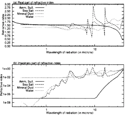
Because the backbone of the new aerosol radiative model is based on Mie theory, figure 4.2 shows the wavelength dependence of both the real and imaginary parts of the refractive index:

(41)

m =n

+

ik (Eq.4.1)

wherem is the total refractive index containing information about the ability of a species to refract(n) and to absorb(ik) radiation. In the visible range, where the bulk(-70%)of the energy exists, the real part of the refractive index is relatively constant but then varies dramatically when the wavelengths of radiation become infrared. As for the imaginary part of the refractive index-in the visible range, only mineral dust has any significant absorbing power, with values of 5 to 6 orders of magnitude greater than all other aerosol constituents. This gap closes, and all aerosol constituents are within an order of

magnitude at the highest modeled wavelengths.

4.1.3 MODEL RUN IDENTIFICATION

For each set of initialization conditions, eight model runs were performed, by varying which atmospheric aerosols were radiatively active in the model. Each model run was given an identification number using the following format:

MMDD_RASM

Where MM is the two-digit month of the simulation (always 09); DD is the two-digit date of the simulation (24 or 25); R is a binary value (0 - off, 1 - on) explaining whether the radiation module is active and A,S, and M are binary values explaining whether the ammonium sulfate, sea salt and mineral dust (respectively) are radiatively active in the model. When R was set to zero, M had a value of 1 or 2 denoting which dust

concentration profile was used on a given day. For the second profile on the 251 \ the

(42)

binary-on value was set to 2 for A, S and M. For example, 0925_1220 refers to the second model run on the 25thof September, with the radiation module active, and both ammonium sulfate and sea salt as radiatively active aerosol species.

4.2 RESULTS FROM PROFILE 1 - 25 SEPTEMBER 2000

For this set (and every subsequent set) of model runs, the analysis of the model output will be confined to four main areas: changes in the temperature profile; changes in the radiation profiles, changes to the vertical velocity profiles, and a discussion about the modeled visibility. This specific case will be covered in much greater detail than the remaining model runs, due to the fact that this set of runs was the baseline for the sensitivity discussion in Chapter 5. For all subsequent sets of model runs, pertinent details will be discussed, with similar results being highlighted and not discussed in great detaiL All of the data presented will be horizontally averaged, excluding the outermost two grid points on either horizontal extent of the domain, using 96 values.

This set of model runs was completed with

Dust Profile #1

the common thread being the initial conditions that were related to the mineral dust profile collected by the SHADE C-130 aircraft from 1501-1518UTC on the 25thof September 2005. The dust profile collected

5000 _4000 E E sooc· 1:: 2' ~2000 1000 400 BOO 1200 16C<l 2000 Conl:er'1ralion (in #km3.1

during this phase of the collection process is illustrated in figure 4.3. The main features of

Figure 4.3: Vertical concentration profile for dust profile #1.

(43)

this dust layer are highly elevated dust concentrations in the 3,000 - 4,500m range, with strong local maxima at 1,750m and ,..,4,350m. The dust concentration averaged between 1,000 and 1,200 partic1es/cm3in the dusty layer, with a profile maximum of 1,889 partic1es/cm3• Using this dust profile and the associated NCEP initialization point (see

figure 4.1), the following discussion highlights the differences caused by the radiative interaction of each of the three aerosol species.

4.2.1 CHANGES IN THE TEMPERATURE PROFILE

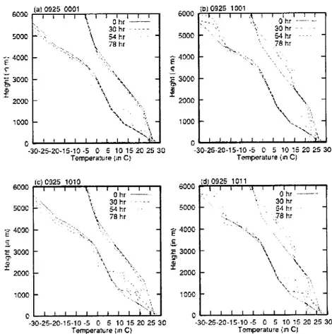
Temperature and moisture profiles are presented for each of the eight model runs in this data set (Figure 4.4). Times chosen for this analysis were the initial time (12UTC), and

1000 --_f: ·~ooo <;-g,3OO0

t

2000 ohr ---30 hr 54 hr 78 hr , 0' '\

\

'\.,... ... . I ...--:..\ ..~-~.~. O~"""'''''....J...I-'''''''-'''l-.J'''''''...L;'''''' -30-25-20-15-10 -5 0 5 1015202530 Temperature (mC) 1000 500e· E4000 £ ~3000

.!

2000 \

\

0 ...--10...- - ' -...1...-...--10... -30-25-20-15-10 -5 0 5 10 1520 25 30 Temperature 11IlC) 6000 ,dl0925 1011 ohr ---30ttr 54hr ]8hr " --.""'1, .-, 5000 1000 E400C' .§, 1:3000 g> :£ 2000 Ohr -30hr 54hr 78hr oL...J~...L...J...I-...I-..I..-l-.J---L-iL:W -30-25-20-15-10 -5 0 5 10 15202530 Temperature l,nC~ 1C<l0 :c3000 V' I 2C<lC·

(44)

0 ..." ...-.:.'-1 ·30·25·20·15·10·5 0 5 1015202530 Temperature 1m Ci o~ ..." ~u ·30·25·20·15·10·5 0 5 1015202530 Temperature (,nCt 6ooC' (e)0925 1100 5000

e-

4000 ';; - 3000 ~

l

2000 1000 Otu \ 30hr---\ SHu \. 78hr 6000 II} 0925 1101 5000 E4000 S; :&3000

:£

2000 1000 ".:..;... oh, 30 h, -54 hr . .78 h, \~

\ , \ \

' \ ' \

...' ... i o ...,,--.... .... ·30·25·20·15·10·5 0 [, 1015202530 Temperature {."C} oL...-J ;....L;-..J ·30·25·20·15-10·5 0 5 1015202530 Temperature (·n CI ..'... ohr .... 30 hr 54 h' 78hr 1000 6000 (ht0925 1111 5000 E4000 ~ E 3000 .'2' ! 2000 ohr . 30 hr 54hr .. 78hr 1000 5OOC' E4000 £ 2;; 3000 <;;> l 2000

Figure 4.4 (panels e-h): Temperature and dew point profiles for model runs from the 0925_0001 family.

18UTC for the next three days, representing 30, 54 and 78 hours of model simulation time respectively, so that successive daytime solar heating events could be tracked.

There are a few things worth noting as it relates to the temperature profile for the no active aerosol case (0925_0001, figure 4.4, panel (a». From the initial sounding, the temperature decreases slightly throughout the lower 4,000m of the model domain. Figure 4.4 only shows the temperature field below 6,000m, because there was essentially no change in temperature field with time above that level. Only very subtle changes occur to the moisture profile below 3,000m, with a general drying of the layers above that. An interesting feature to note is the development of a temperature inversion/moist layer that

(45)

grows in height with time. By the end of the model run (78 hours), the cloud base is at 1,600m. This value is quite high, and is rather unreasonable for the height of a marine boundary layer. This issue will be addressed in the sensitivity study in Chapter 5, with the results here taken as is, with the understanding that there is a lack of realism presented by these results.

Radiatively active aerosols within the model bring changes in the temperature and moisture profiles-some are subtle, others are hard to miss (figure 4.4, panels b-h). When looking at the effects of ammonium sulfate, there is only one readily apparent effect- it seems to keep the boundary layer from growing. In all four cases where ammonium sulfate is active, the temperature and moisture inversion is lower than during

I;";'Dust Only - 30 hrs (b> Dus1 and Salt,30hrs

16000r---r---r--;r--.,...--.,---,-,--..., 0925 1001 14000 HaDe· 0925 1010 0925 1011 6000 12000 -e-10000 Ii ~. 800e·

l

60:30 4000 .I "'-. ₁₂₀₀₀ E1000e, s .E 8000

'"

:f

4000 ..\.... " 2000

,"

{

C.I - -...;:.I...I~.I-...- - I _...J -4 -2 0 2 4 6 B 10 12

Temperature Olflerence (inC~ (c.l DustandAmmm1lum Sulfate -3C' hrs

16000r--,..~--,r---r-..,..--,-,...,

2000

e'--...L..--l-...I~...- - I _...J

-4 ·2 0 2 4 6 8 10 12

Tempilraturll Oi'ference :in GI (ell Ous1wlb-~thSaa and P.mm S'JIf. ,30 hrs

16000 r--..,-~--,r---r-..,..--,-,..., 14e<l0 12000 09251'00 -.-., 0925 1'01 14000 12000 0925 1110 0925 "11 E1000e, E"10000 ~ ,~ :E BOOO 1: 8000 )l' Q': 1 6000 1,:__ :f _&000 -L 400e, 4000 " , 2000 ~- 2000 J .•"'

.-_.c' OL-....L.--"'----''--...--'---'-_.L..-~ -4 ·2 0 2 4 6 8 '0 12

Temperature OiHerence (in C>

OL---'---'-_'--....L.---'----''--...~

-4 ·2 0 2 4 6 8 10 12

Tempilratufl'lOi~ference:,nCI

(46)

the corresponding runs without ammonium sulfate. Aside from that, there is very little to speak of as an ammonium sulfate effect on either temperature or moisture. Nearly the same thing can be said of sea salt, but with one major difference-in all four runs containing the sea salt radiative effect, the inversion layer is markedly higher than corresponding runs without sea salt as radiatively active. Again, there are very small, if any, noticeable temperature and/or dew point profile changes as a result of having sea salt radiatively active.

There are two effects from the radiative activity of mineral dust that are apparent in figure 4.4. The first is that the mineral dust, in general, suppressed the growth of the

(a) DustOnly - 78 hrs

16OOC,r----r---r.,--.,----r----,.,---r---r-..

(b~Dust and Salt - 78 hrs

14000 12C<l0 E1000D \; ~ 8ooC'

l

6000 14000 12000 E10aOO \; ~ 8000 ~ &000 4000

,-

. 0925 1010 . 0925 10'11 ...-.--2C'Ol) 2000 C 0 -4 -2 0 2 4 6 8 10 12 ·4 ·2 0 2 4 6 8 10 12

Temperature Di1ierence (in Cl Temperature Dilferer1ce !,Inq (c,l Dust and Ammoruum Sulfate - 78 hrs (til DustwlbolhSalt and Amm. S'JIf. - 78 hrs

16OOC' 16000 0925 1100 . . . ,, _{0925 1110} 14000 0925 1101 14000 ,, 0925 1111 12000 12000 E' 10ooC' E10000 ~ ,£

=

800D ...,,~. _1: ₈₀₀₀ 2' ,2' 1. 600D ~ 6000 4000

..

...::--~ 4000 .- -2ooC' .~- 200C-

-,'

D C--4 -2 0 2 4 6 8 10 12 -4 -2 0 2 4 E 8 10 12

Temperature Diflerence (inq Temperature Di!ference l;n C,l

(47)

mixed layer. However, the main aerosol effect that is seen through the temperature field is the dramatic heating in the highly concentrated dust layer. The magnitude of this effect with time can be seen in figures 4.5 and 4.6. After 30 hours of simulation time (two daytime periods), a maximum heating of 6°C is seen at 4,000m, and at 78 hours, the difference from the run with no radiatively active aerosols is overWoe. Again using

figures 4.5 and 4.6, small changes in the temperature profile are observed with the other two aerosol species, but nothing as pronounced as is seen when the dust layer is present. In general, the inversion layer is also suppressed by the presence radiative presence of mineral dust.

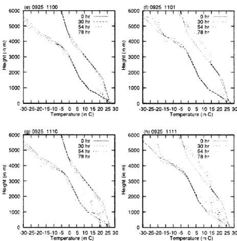
4.2.2 CHANGES IN THE RADIATION STREAMS

In order for the previously described temperature changes to occur, changes must also have been made to the radiation streams within the model. Because the changes to the radiation streams are immediate, the magnitudes of the irradiances will be shown for only two times, the initial time (12UTC) during nearly overhead sunlight, and 12 hours later (OOUTC), with no sunlight present. As previously stated the model contains three solar bands with modeled wavelengths from 245nm to 4.641J,m and five infrared bands ranging from 4.641J,m to 401J,m. Figure 4.7 shows the simulated upward and downward

irradiances for both the shortwave and longwave radiation in the model at 12UTC for all eight different aerosol representations. Again, there are a few subtle differences in the eight different panels on figure 4.7. There is no discemable change to the radiation field caused by the presence of ammonium sulfate. Only one subtle change is evident with the radiative treatment of sea-salt-a slight increase in downwelling longwave radiation near

(48)

16000 l.alOn50001-0 h,

•

, •

_·

• , 1

•

\ I l , • \"'l \ \, , •, 2000 4000

1&000 ,:i;:.bJ:..;0:.:9;;.2::;5.,..1.:.,:O;.:0:.:.1_-..:0,:.h::.r- r - - - ,...,... SW-UP 14000 SW· ON LIN· UP LW ON -oL-....J_..lJ...IL_.l-_L-...l....J o 200 400 600 800 1000 1200 frradJance {mWim2:1 12000 ElOOOO !i ~8000

i

6000 SW-UP SW·ON LW·UP LW· ON ----200 400 600 800 1000 1200 Irradiance (in W/m2/ 2000 4000 14000 - 8000 -§,

l.

6000 SW-UP SW·ON LW-UP LW· ON -SW·UP SWoON LW-UP LW ON -• "

_·

i~ \ 1 l I I

•

_" \, , •

.

\, \ 200C 4000 1400C 2000 Ol!----l_~'--..I!...--l_ _.L._.J-J o 200 400 600 800 1000 1200 lrradiance Ii"W/m21 16000 (fl0925 1101 - 0 hr

I

12000 Eloooe ~ -£,8000

-l.

6000 14000 ol:....---l_..I.L.'--...IL.._L....•...L_....L...J o 200 400 600 800 1000 1200 irraa.ance 1mWlm2) 4000 16000 ,ell0925 1011 - 0hr 12000 E10000 .E J: 8000 !2' :'i 600C \ \ ~ ~_, \

·

•I, : , i \ \ \ \

•

, \ \ \ 14000 16000~..::.::~..;l~0r.:ol0:::..;.-::,0;.:.h:..r-.,...-.,_-..., SW-UP SWoON LW·UP LW·DN 4000 2000 o"'----l--il...'--..l---'L.-..L.I._....L...J o 200 400 600 800 1000 1200 Irradiance (in W/m2f QLC-...L----'l...L.-'_.1.----l_Ll..._.J...J o 200 400 600 800 1000 1200 Irradlancefir. W/m21 12000 El0000 ~, :E8000 .;;> 1. 6000 4000 El000e C;; - 8000 -§,

1.

6000 200 400 600 80e· 1000 1200 !rradiance ,mW/m2.1 " ;,

..

_,

•

I

·

•

_·

,, \, \ \

..

\ o1L'_....J.._...u..-,-..ll:"""....J.._....L._....L...J o 4000 2000 14000 16000p';.:.h:..;10::.::9r-2::..5..;1~1,:.11.:...;.;.O:,:.::hr_..-._...-~,...., SW-UP SWoON LW-UP LW ON -12000 ElOOOO ,.§: J: 8000 2' :£ 6000 SW-UP SWoON LW·UP LW-DN I • \1_,I

1

\ 1, \ ,

·

\, , \ \, '. \, , 16000 I10925 1110 - 0 hr 4000 14000 o"'-...J._:'-l..I....-...1---''--.L.l.._....L...J o 200 400 600 800 1000 1200 Irradlance (inW./m2.1 2000 12000 E10e<JO

"

:E 8000 <;(' 1.6000

(49)

the surface. The most obvious changes to the modeled irradiances are manifested with the presence of mineral dust. Downwelling solar radiation is dramatically reduced to a surface irradiance value of 618 W/m2from 947 W/m2when dust is not present.

The change in nighttime radiation streams due to the radiative activity of aerosols is much less drastic than the effect during the daytime (figure 4.8). Again ammonium sulfate causes no immediately discernable changes in the radiation streams. The sea salt however causes one large change-a drastic and sudden increase in downwelling longwave radiation at 300m (e.g., figure 4.8, panel c). This change is indicative of the formation of a low-level cloud. The presence of mineral dust does cause an increase in

4000 12000 4000 OL-.--"'-...- ..._ ...--""-... o 100 200 300 400 500 600 irrad1ance\InW/m2:1 .2000 16000nlb~·I..:;;09:;:2:::.5...;1..:;;00T1:...;.'=,2;.:.:hr_-r-_,.---, ~SW.UP •. _SWDN -'UN·UP \ LW· DN

---.

\, \ •,_, \

·

•

I

.

"""'" " \. 14000 12000 E10000 s: :E 8000

'"

~ 6000 0 ...- ...- ...- -... o '00 200 30e 400 500 600

Irradiance (inWIm2> 16000 tal 0925 0001 - 12 hr .i 'OW-UP 'I ..., 14000 • SW ON -LW-UP LW -ON .----E10000 ~ F 8000

'"

!

6000

\

•\

.

\ \ \

.

•

_·

•

_•_, ", ...,..., 2000 " .. oL - - - - L _ - - ' - _...

_'.:.;:.-=

...

--'--~ o 100 200 300 400 50'0 600 Irradlance,mWim21 4000 12000 16000 ",;d-.'1-.09"'T2;.;.S;..1-.0,.'1;..-_';;;2i"'hr_-r-_,.----, SW·UP 'SWoON -LW-UP - ,-J...W, ON ---14000 - E10oo0 ~ 1:' 8000 ~ ~ 6000

-'00 200 300 400 500 600

Irradiance (inWIm2l

, '.

.

,_, , ••_•

_.

, " , ~, "

.

", . CU - - - I _ - - ' - _ - I . ...;;:.;--:.:;-=...-,"-.1.---' o ·\000 .2000 1";000 Ic,0925 1010·12 hr • • SW-UP --14000 ~ $W DN -I LW - UP - --. 12000 LW,ON ---f'10000 §. 'E 8000 ¥'J I 6000

Figure 4.8 (panels a-d): Short- and longwave radiation streams for model runs containing the 0925_0001 family after 12 hours of simulation time.

Addition of the direct radiative effect of atmospheric aerosols into the Regional Atmospheric Modeling System (RAMS), The

000 Center for Geosciences/Atmospheric Research under grant

DAAD19·02·2·0005

THE ADDITION OF THE DIRECT RADIATIVE EFFECT OF

ATMOSPHERIC AEROSOLS INTO THE REGIONAL

ATMOSPHERIC MODELING SYSTEM (RAMS)

by David Stokowski

ABSTRACT

ACKNOWLEDGEMENTS

u.K.

TABLE OF CONTENTS

CHAPTER 5 - SENSITIVITY STUDIES...

60

CHAPTER 6 - CONCLUSIONS...

70

CHAPTER

1 -

INTRODUCTION

CHAPTER

2

-THE MODEL

"

•

•

•

=

=

=

=

*

*

CHAPTER

3

-THE SAHARAN DUST

EXPERIMENT

?

r

*

w

..

!

i

"w,

CHAPTER

4

-THE MODEL

'e-

£'

..,',

t

...

,/S:-~'.~._.:::;/~{ .'~,-<~.~/~;~~'~'~;y~

:"

+

t

\

.!

\

e-

l

:£

\ , \ \

' \ ' \

l

'"

:f

,"

{

l

,-

=

..

-,'

•

·

•

i

l.

·

•

_·

_·

_·

_·

_.