The Relationship Between the Price of Oil and Unemployment in Sweden

J

I

B

S

JÖNKÖPI NG UNIVER SITY

T h e R e l a t i o n s h i p B e t w e e n t h e

P r i c e o f O i l a n d U n e m p l o y m e n t

i n S w e d e n

Paper within Economics Authors: Hannes Mellquist

Kanditatuppsats inom nationalekonomi

Titel: Sambandet mellan oljepriset och arbetslösheten i Sverige Författare: Hannes Mellquist och Markus Femermo

Handledare: Professor Scott Hacker och Doktorand James Dzansi Datum: Januari 2007

Ämnesord: Arbetslöshet, oljepriset, granger causality, Sverige

Sammanfattning

Oljeberoendet i världen har stigit i takt med den ökade industrialiseringen och olja har orsakat såväl kriser som krig. I arbetet undersöks oljeprisets inverkan på arbetslösheten i Sverige. Det är intressant att studera förhållandet i Sverige då det finns skillnader när det gäller arbetslöshet och ersättningssystem jämfört med andra industrialiserade länder. Syftet med uppsatsen är att se om en förändring i oljepriset kommer att påverka arbetslösheten vid en senare tidpunkt. Vi genomför en linjär regression och Grangers kausalitets test för att se om det finns ett samband.

Resultatet från våra regressioner tyder på att det existerar ett samband mellan priset av olja och arbetslösheten i Sverige. Vi kan inte bevisa att en ökning av oljepriset kommer leda till en positiv eller negativ förändring av arbetslösheten eftersom de estimerade koefficienterna i kausalitets testen är både positiva och negativa.

Bachelor thesis within economics

Title: The relationship between the price of oil and unemployment in Sweden

Authors: Hannes Mellquist and Markus Femermo

Tutors: Professor Scott Hacker and PhD Candidate James Dzansi Date: January 2007

Subject terms: Unemployment, oil price, granger causality, Sweden

Abstract

The dependence on oil has increased in many nations as a result of increasing industrialization and oil has been the factor of many crises as well as many wars. This paper examines how the price of oil affects the unemployment in Sweden. The case of Sweden is interesting since its politics are very different compared to other industrialized countries when it comes to unemployment and benefits. Our main objective is to see whether a change in the oil price will cause a change in unemployment at a later stage. We perform linear regression analysis relating current changes in the variables and Granger causality tests to conclude if there exists a direct relationship.

The result we received from our linear regression test on current changes and our Granger causality test showed a relationship between the price of oil and unemployment in Sweden. In the linear regression relating current changes in these variables, a positive relationship was indicated. Due to the fact that some of the coefficient estimates are positive and some are negative in the Granger causality regressions, we can not conclude whether an increase in the price of oil will cause a positive or negative effect on unemployment.

Table of Contents

1

Introduction... 1

1.1 Purpose ...2

1.2 Outline ...2

2

Background... 3

2.1 Oil price fluctuations prior to 1973 ...3

2.2 SOPI and NOPI ...4

2.3 Oil consumption...4

2.4 Unemployment ...5

2.4.1 Unemployment benefits...5

2.4.2 Unemployment in Sweden...6

3

Theoretical Framework... 8

3.1 Equilibrium unemployment model ...8

3.2 Granger causality ...9

4

Empirical work ... 11

4.1 Data...11

4.2 Linear regression...12

4.3 Granger Causality Test...14

5

Analysis ... 15

6

Conclusions and Suggestions for Further Research... 17

References ... 18

Appendices

Appendix 2 – Granger test calculations...21

1 Introduction

The importance of oil in our daily lives is well known and especially when it comes to transportation. Oil is a unique commodity because of its importance and its effect on the world economy. The largest oil region in the world is the Middle East, a region that has problems with terrorists, wars, and dictatorships. Since the countries in the Middle East control most of the supply of oil in the world this affects the way oil dependent countries maintain their relationship to these countries. Oil is therefore a political instrument that has to be treated carefully. The Organization of Petroleum Exporting Countries (OPEC) controls the largest oil supplies which gives it a huge power and it can control the supply and price of oil. In 1973 OPEC decided to cut oil production which resulted in almost a tripling of its price and the developed countries were sent into recession (Bade & Parkin, 2003).

History has shown that oil price shocks have led large economies into great recessions, e.g. 1973, but can we find evidence that the price of oil affects unemployment in a smaller economy?

Most of the earlier work concerning the connection between the oil price and unemployment has been done using US data. In this paper we are using Swedish data which might give a different result since countries usually measure unemployment in different ways. Even though almost every country in the world is dependent on oil the dependency differs from country to country. An average American consumer uses a lot more oil per year than an average Swedish consumer. So an increase in the price of oil might have a worse effect on the US economy compared to the Swedish economy.

The government in Sweden has to deal with many issues to create economic growth and will always have to be aware of fluctuations in the price of oil. To avoid recessions they have to follow the price of oil and make decisions depending how it is moving. The price of oil is of course not the only factor they are looking at, but it is an important part of the economy.

Swedish industry is also dependent on oil and when the price increases, this can have a major effect for their production. Many major Swedish industries have threatened to shut down production within the Swedish boarders due to the propositions of higher tax on gasoline made by the politicians. So if the price of oil increases, Swedish companies will leave for lower production-cost countries and will force the unemployment rate in Sweden to go up.

In this thesis we are going to examine the relationship between the price of oil and the unemployment rate in Sweden. It is important to understand this relationship since it reflects on the sensitivity of the Swedish economy to changes occurring in the volatile Middle East. So a decision in Saudi Arabia to lower the supply of oil during a period of time, for example, might force people in Sweden into unemployment a year later.

1.1 Purpose

The purpose of this thesis is to test if there exists a relationship between unemployment and the price of oil using Swedish data from 1980 to 2004. We will test whether the oil price Granger causes unemployment.

1.2 Outline

In section 2 there is a presentation concerning the price of oil and its influence on unemployment. Earlier work will be presented and discussed to show what has been done in this subject earlier. In section 3 a theoretical framework will be discussed and Granger causality will be presented since we will use it in our regressions, and it is an important part in the study of this subject. In section 4 we will use some of the theoretical framework to do our empirical work. We will use data of the Swedish unemployment and the price of oil averaging from three markets, USA, Europe and Asia. The oil price is adjusted for inflation. In section 5 we will present our analysis and in section 6 we will end up with our conclusion.

2 Background

2.1 Oil price fluctuations prior to 1973

There is a lot of research done in the field of oil prices and their impact on the macroeconomy. One of the first to examine the relationship between the change in price of oil and the way it affects the macroeconomy was James D. Hamilton. In 1983 he wrote a paper concerning this issue using U.S. data. From his empirical work he found a positive relationship between the increase in the price of oil and recessions in the U.S. since World War II. Even though he could not say that the increase in the price of oil was the only reason for the recessions, the correlation was statistically significant. He estimated that the U.S. economy turned into recession after around 9 months after an oil price shock. In his paper Hamilton had three different hypotheses that he worked with to explain the correlation.

- Hypothesis 1: The correlation represents a historical coincidence; that is, the factors truly responsible for recessions just happened to occur at about the same time as the oil price increases.

- Hypothesis 2: The correlation results from an endogenous explanatory variable; that is, there is some third set of influences that in fact caused both the oil price increases and the recessions.

- Hypothesis 3: At least some of the recessions in the United States prior to 1973 were causally influenced by an exogenous increase in the price of crude petroleum (Hamilton, 1983, p.230).

Hamilton (1983) used data from the period 1948-72 in his econometric work. With his first hypothesis he had to reject the null hypothesis of no relation between the oil price increases and the recessions. So now he knew that there must be a systematic relationship since there was no evidence for a historical coincidence.

After he had tested his second hypothesis he determined that there was no third set of influences from the ones he was considering, that could have been the reason for both the oil price increases and the following recessions. To test this hypothesis he used six different macroeconomic variables; real GNP, unemployment, implicit price deflator for non-farm business income, hourly compensation per worker (wages), import prices and money supply. None of these variables, single or collectively, showed any behavior that could have caused the oil price to increase in such a way as it did. He looked at these variables a year prior to the oil price shocks.

Since Hamilton rejected both the first and the second hypothesis he gained more evidence to support the third hypothesis, that some of the recessions between 1948-72 were caused by an increase in the price of oil. There is however not enough evidence to claim that an increase in the price of oil was necessary or a sufficient condition for the recessions. "Nor is it to assert that this correlation should be viewed as an immutable structural relation. Changes in expected inflation, the response of monetary policy to oil shocks, or the regime in which oil prices are determined could be expected to give rise to a different dynamic pattern”(Hamilton, 1983, p.247).

2.2 SOPI and NOPI

Mark A. Hooker wrote a paper in 1999 in which he used Hamilton’s work, but made some changes. When it comes to output he uses the changes from one year to another instead of every quarter and he argues that this is smoother. In his equations he excludes variables like inflation and interest rates.

Hooker´s result when studying the oil price series were divided into Scaled Oil Price increases(SOPI) and Net Oil Price Increases(NOPI). The result that one gets from SOPI is that an increase in the oil price might not be proportional to the size of the shock. It does not have to be independent from a shock in another time period. A price shock that is small will be scaled up if it happens in a calm period and scaled down in a period that is volatile. With NOPI one looks at the influence the shock has in a threshold way. If the shock does not bring the oil price up above previous years high it is scaled down to zero. Hooker wanted to test if SOPI and NOPI Granger cause output or unemployment and he found that asymmetric and nonlinear oil prices predict output, but not unemployment. When he used the real oil price level SOPI and NOPI predict unemployment but not output. According to this result different transformations of oil prices seem to affect unemployment and output (Hooker, 1999).

Lee, Ni & Ratti (1995) also express a similar result comparable to NOPI. They considered the role of price variability and argue that the change in the oil price should have a greater impact on real GNP in an environment where oil prices have been stable, compared to environments where oil prices have been unstable.

From their work they found that positive normalized oil price shocks are highly significant, while negative normalized oil price shocks are not statistically significant. This means that positive normalized shocks in real oil prices have a strong relation to negative real growth and negative normalized shocks in real oil prices are not significant (Lee, Ni & Ratti, 1995).

2.3 Oil consumption

The economic growth in large population countries, for example China and India, have put even greater pressure on oil demand than ever before. An average person in China and India consumes 1.7 and 0.7 barrels per person and day, compared with an average person in the U.S. and Sweden who consumes 25 and 13 barrels respectively. We expect that the average consumption in China and India will increase in pace with the growth but if this will ever occur the production of oil will have to increase substantially. Of 65 oil producing countries, 54 are already at their production peak and another five are expected to reach their peak in the next six years. The total world production is expected to reach its maximum in the next 20 years. It is only in the Middle East where the production of oil can be increased, but in order to keep the price at a high level they aim to have production at an even pace (Vetenskapliga argument i energidebatten, 1995).

There exist alternatives to oil which are planned to substitute the oil consumption in the long run. Some examples are wind power, solar power, tidal power, hydropower, methanol and ethanol (Energimyndigheten, 2003). The problem today with the alternatives is that the price is too high compared to the price of oil.

2.4 Unemployment

There are four types of unemployment: • Cyclical

• Frictional • Seasonal • Structural

Cyclical unemployment varies with recessions and expansions in the economy. It increases during a recession and decreases during an expansion. Frictional unemployment is unemployment that occurs from normal labor turnover. People who leave and enter jobs and the creation and destruction of jobs are part of frictional unemployment. This type of unemployment is permanent. Seasonal unemployment occurs because of the change in weather and other annual events from one season to another. If you are working as a ski teacher you are only working in the winter and during the summer you will experience seasonal unemployment. Structural unemployment occurs because of changes in technology or international competition. Some jobs disappear because of new technology and therefore people need to look for other jobs and sometimes improve their skills (Bade & Parkin, 2003).

Full employment occurs when unemployment consists only of structural, seasonal and frictional unemployment. When there is full employment the unemployment rate is called the natural unemployment rate (Bade & Parkin, 2003).

The calculated unemployment rate is the number of people unemployed divided by the size of the labor force.

2.4.1 Unemployment benefits

There are two ways in which unemployment benefits increase the unemployment rate. First, longer job search is allowed. If an unemployed person receives unemployment benefits it will give him the opportunity to look for a job during a longer period. Second, with unemployment benefits, the consequences of being between jobs are less severe. So the firms and the workers are less interested in creating a stable employment. Unemployment benefits increase the replacement ratio, which is the proportion between after-tax income while unemployed and the after-tax income while employed (Dornbusch, Fischer & Startz, 2004).

2.4.2 Unemployment in Sweden

At the beginning of the 1990´s the unemployment rate increased to a high level in Sweden. At the end of the 1980´s the inflation rate in Sweden was very high, and salaries and prices were increasing at a higher level compared to other developed countries. High salaries made Sweden less competitive and the industry production decreased by almost 10% from 1990 until 1992. An increase in the interest rate made it more expensive to borrow money and the savings rate went up. The increase in savings created a decrease in consumption, especially for domestic products. The politicians changed their economic policy to focus on the inflation rate instead of the unemployment level (Forslund & Holmlund, 2003).

In 2006, 37000 Swedish students were searching for a job according to statistics from SCB. This group of people is in most countries included in the unemployment rate, but this is not the case for Sweden (SCB, 2006).

In late 1992 Sweden was in a great recession. A reform was necessary to stabilize the Swedish economy. Monetary policy based on inflation targeting was at that time a relatively new phenomenon and there were many doubts on how the reform would work in Sweden. The 19th of November 1992 is considered a milestone for the Swedish Riksbank, when the fixed exchange rate was abandoned. The reform was followed by large currency outflows and an extreme interest rate hike in an attempt to protect the Swedish Krona (Heikensten, 1999). Unemployment 0,0000 1,0000 2,0000 3,0000 4,0000 5,0000 6,0000 7,0000 8,0000 9,0000 10,0000 1 9 8 0 Q 1 1 9 8 1 Q 4 1 9 8 3 Q 3 1 9 8 5 Q 2 1 9 8 7 Q 1 1 9 8 8 Q 4 1 9 9 0 Q 3 1 9 9 2 Q 2 1 9 9 4 Q 1 1 9 9 5 Q 4 1 9 9 7 Q 3 1 9 9 9 Q 2 2 0 0 1 Q 1 2 0 0 2 Q 4 2 0 0 4 Q 3 U n e m p lo y m e n t ra te ( % )

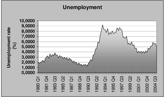
Figure 2.1 Unemployment rate in Sweden 1980-2004

Figure 2.1 displays the unemployment situation in Sweden during the 1980-2004 period. The rapid increase in unemployment that occurred in Sweden in 1992 can clearly be seen.

The governmental actions in 1992 that led to a high increase in unemployment can be explained by the Phillips Curve in figure 2.2, according to which there exists an inverse correlation between inflation and unemployment. When unemployment is high, inflation is low and when inflation is high, unemployment is low. It is important to note that the relationship can only be verified in the short run. In the long run, there seems to be no correlation between inflation and unemployment (Bade & Parkin, 2003).

3 Theoretical Framework

3.1 Equilibrium unemployment model

In 1998 Alan Carruth, Mark Hooker & Andrew Oswald (C, H & O) modified the Shapiro & Stiglitz (1984) model by adding a role for input prices to create an equilibrium unemployment model. In the C, H & O model, equilibrium unemployment, U*, is a function of five variables, as shown in the following equation:

U* = U*(r, p₀, b(µ), e, d), where,

r = interest rate p0 = price of oil

b(µ) = level of unemployment benefits e = on-the-job effort

d = probability of successfully shirking at work

According to the model, an increase in any of these five variables has a positive effect on U*, all else equal, with the exception of an increase in d, which has a negative effect. According to their logic, an increase in the price of oil will lead to less profit for the firms. To get back to zero-profit equilibrium one of the variables has to change. Since interest rates are largely fixed internationally, the price of labor has to alter. Considering unemployment and wages to be connected inversely by a no-shirking condition, equilibrium unemployment must rise. This is the only thing that will make the workers accept a lower salary. So unemployment will rise because of an increase in the price of oil.

3.2 Granger causality

Regression analysis constitutes the dependence of one variable on other variables but this does not automatically imply causation. The relationship between variables can not prove causality or the direction of influence.

It is different when we are dealing with time-series data. The time-series can not run backwards, for example, if event A happens before event B it can be that A causes B, but it is impossible for the other way around to occur. This is how the Granger causality test can be explained (Gujarati, 2003).

Granger causality (Granger 1969) is built up to evaluate the forecasting ability of one time-series variable by another. The effect can rule out that one variable is causing another by the idea that for an event to cause another event, it must at least precede it. By this reason this is probably as close as we can possible get in using data analysis to evaluate the concept of causality (Granger, 1969).

Lütkepohl (1993) found evidence for new theory of multivariable models. The vector of numeral variables Z is used in the addition to the variables of interest, X and Y, and it is possible that Y does not cause X in this case but can still calculate X for several periods ahead (Dufour & Renault, 1998).

We will now assume that the information set Ft has the form (xt, zt, xt-1, zt-1,...,x1, z1), where x and z are vectors and z may or may not include other variables than y. xt is Granger causal for yt with respect to Ft.. We can say that xt is Granger causal for yt if xt helps predict yt at some stage in the future.

There will often be cases known as “feedback systems”. In these cases xt Granger causes yt and yt Granger causes xt. Granger causality is basically assumptions about linear prediction, investigating if one thing happens before another so each test of Granger causality only considers Granger causality in one direction (Toda & Phillips, 1994).

Granger causality is often used to test the relationship between changes in oil prices and macroeconomic variables. When Hamilton wanted to show in his paper from 1983, that changes in the oil price affected the US GNP and unemployment rate he used Granger causality. In his work he used data until 1980 and he found that the oil price Granger caused U.S. GNP and the unemployment rate with bivariate equations and 6-variable equations (Sims, 1980). There are different opinions concerning the influence of the oil price changes on the economy. Lee, Ni and Ratti (1995) and Ferderer (1996) have the opinion that what matters are the measures of oil price volatility. Morks opinion is that only increases in the oil price have an influence on the economy.

When C, H & O wanted to test whether oil prices Granger cause unemployment they divided the entire sample into two subsamples. The entire sample (1954-1994) was divided into two subsamples with the split occurring at 1972-73. They used fairly long lags of 8 quarters in the subsample tests and 12 lags in the full sample tests. According to their results, real oil prices Granger cause unemployment.

Therefore, compared to what Hooker found before, oil prices still Granger cause unemployment in samples that include 1980´s and 1990´s data. C, H & O argue that the reason why there is a difference between their results and other research is the inclusion or exclusion of money market variables like Federal funds rates or Treasury bills. According to C, H & O there are two possible explanations. “The first is that oil prices do not affect the macroeconomy, but appear to do so because of their comovement with monetary policy, as Bohi (1989) has argued.... The second is that money market variables-due to Fed policy and to private sector expectations-now systematically respond to oil price changes, and so oil price effects now appear weaker due to multicollinearity”(Carruth, Hooker & Oswald, 1998, p.11).

4 Empirical work

4.1 Data

To be able to answer the question whether oil price changes Granger cause the unemployment level in Sweden we had to find the necessary data. The data ranges from quarter one in 1980 until quarter four in 2004.

The oil price we found is an average price from three markets; the U.S., European and Asian markets. The currency was in dollars so first we had to change the price into Swedish crowns(SEK) by using the exchange rate. The price of oil also had to be adjusted for inflation which we did by using the Swedish Consumer Price Index(CPI).

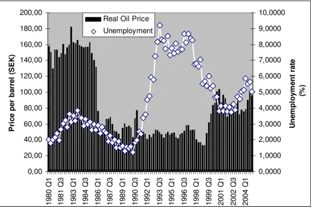
In figure 4.1 the change in the real oil price and unemployment rate from 1980 until 2004 is shown. During the beginning of the 1980´s the price was quite high, but at the end of 1985 the drop was extensive. After 1999 it stayed at a relatively even level except for some small ups and downs. After a big increase in 1999-2000 it has again stayed at a relatively even level. In the graph below it is shown how the price of oil and unemployment follow each other up to 1992 where unemployment increased drastically. We excluded the years between 1991-1992 from our regression tests since the big changes in unemployment during these years, caused many outliers.

0,00 20,00 40,00 60,00 80,00 100,00 120,00 140,00 160,00 180,00 200,00 1 9 8 0 Q 1 1 9 8 1 Q 3 1 9 8 3 Q 1 1 9 8 4 Q 3 1 9 8 6 Q 1 1 9 8 7 Q 3 1 9 8 9 Q 1 1 9 9 0 Q 3 1 9 9 2 Q 1 1 9 9 3 Q 3 1 9 9 5 Q 1 1 9 9 6 Q 3 1 9 9 8 Q 1 1 9 9 9 Q 3 2 0 0 1 Q 1 2 0 0 2 Q 3 2 0 0 4 Q 1 P ri c e p e r b a rr e l (S E K ) 0,0000 1,0000 2,0000 3,0000 4,0000 5,0000 6,0000 7,0000 8,0000 9,0000 10,0000 U n e m p lo y m e n t ra te ( % )

Real Oil Price Unemployment

4.2 Linear regression

First we did a simple linear regression with the change in unemployment as the dependent variable and the change in the oil price as independent variable to see if there was a relationship between them. We used seasonal dummy variables since there is a seasonal pattern and we wanted to avoid this factor in our regressions. The regression equation estimated is:

∆Ut = α + β ∆Poilt + γ1D1 + γ2D2 + γ3D3 + εt , where,

Ut = unemployment rate Poilt = price of oil

D1 = 1 if second quarter, otherwise 0 D2 = 1 if third quarter, otherwise 0 D3 = 1 if fourth quarter, otherwise 0

∆ is the first-difference operator and ε_t is the error term.

The results of this estimation are shown in table 4.1. To test whether there is a relationship between unemployment and the price of oil we set up two hypotheses. In the null hypothesis β is equal to 0 and the alternative hypothesis is that β is not equal to 0. The p-value for the ∆Poil coefficient estimate is 0.007 which means that we can reject the null hypothesis at the 1% significance level (0.01>0.007). By rejecting the null hypothesis we can conclude that there is a relationship between the change in the oil price and the change in the unemployment level. That relationship is estimated to be positive.

Table 4.1 Linear regression results with change in uemployment rate as dependent variable

MODEL Unstandardized Coefficients Significance

B Std. Error Constant -0.089 0.019 0.000 ∆Poil 0.184 0.067 0.007 D1 0.165 0.027 0.000 D2 -0.015 0.026 0.582 D3 0.232 0.026 0.000 R2 = 0.621

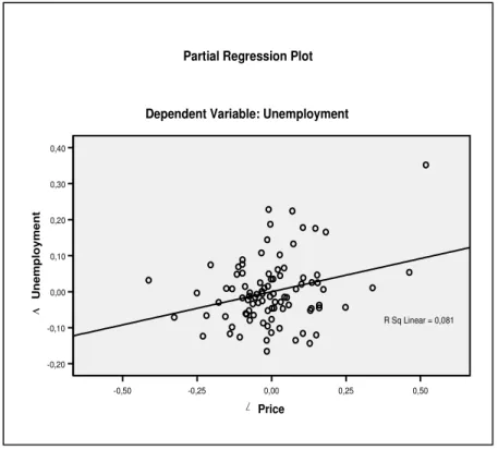
The partial regression plot shown in figure 4.2 plots two residuals against each other: the residuals from ∆U regressed against the dummy variables with intercept, and the residuals from ∆Poil regressed against the dummy variables with intercept. The positive relationship between ∆U and ∆Poil, after controlling for seasonal effects is shown visually.

0,50 0,25 0,00 -0,25 -0,50 Price 0,40 0,30 0,20 0,10 0,00 -0,10 -0,20 U n e mp lo y me n t

Partial Regression Plot

Dependent Variable: Unemployment

R Sq Linear = 0,081

∆

∆

4.3 Granger Causality Test

The general equation that we will be focusing on for our Granger Causality analysis is:

The change in the price of oil and the change in unemployment with data from different periods in time have to be included to test whether oil price changes Granger cause unemployment rate changes. Dummy variables are also included to even out the seasonal patterns. An error term is also added.

By doing F-tests we were able to choose the correct number of lags to be used in the Granger test. We began to use 5 lags (m=5) in the unrestricted regression and then we used lower values for m until βm=δm=0 could be rejected at the 5% significance level. From the lag tests we found out that the optimal number of lags to be used for the causality test to be 4 (see appendix 1). When we knew how many lags to use, we could do our causality test where the restricted regression did not have any lags for the price of oil. Below we present the two regressions used for our Granger Causality analysis:

Restricted regression Unrestricted regression

∆Ut = α0 + α1 ∆Ut-1 ∆Ut = α0 + α1 ∆Ut-1 + α2 ∆Poilt-1

+ α3 ∆Ut-2 + α3 ∆Ut-2 + α4 ∆Poilt-2

+ α5 ∆Ut-3 + α5 ∆Ut-3 + α6 ∆Poilt-3

+ α7 ∆Ut-4 + α7 ∆Ut-4 + α8 ∆Poilt-4

+ α11D1 + α12D2 + α11D1 + α12D2

+ α13D3 +εt + α13D3 +εt

Table 4.2 Restricted regression, ANOVA

Model

Sum of

Squares df Mean Square F Sig.

Regression 1.129 7 .161 20.306 .000(a)

Residual .627 79 .008

Total 1.757 86

Table 4.3 Unrestricted regression, ANOVA

Model

Sum of

Squares df Mean Square F Sig.

Regression 1.194 11 .109 14.476 .000(a)

Residual .562 75 .007

Total 1.757 86

The null hypothesis in our Granger test is α2=0, α4=0, α6=0, and α8=0. Our calculated F-value turned out to be 2.1686 which means that we can reject our null hypothesis at 10% significance level (2.1686>2.04) (see appendix 2). The result from this test is that the price

(

)

∑

5 Analysis

The result from our empirical analysis indicates that there exists a relationship between the price of oil and unemployment in Sweden. Due to the fact that some of the coefficients are positive and some are negative, we can not conclude whether an increase in the price of oil will cause a positive or negative effect on unemployment.

By using dummy variables in our linear regression test, we were able to even out the seasonal patterns that before made our result insignificant. The seasonal patterns could be explained by, e.g. seasonal unemployment due to shifting weather. Our significant result was found by ignoring the years of 1991-1992 in which outliers were found and the usage of dummy variables.

Regarding the Granger causality we wanted to test if the price of oil cause unemployment and that it is not the other way around. But consider this case of Christmas. We have stated in the theory above that if event A happens before event B, it can be that A, causes B, but it is impossible for the other way around to occur. Christmas Eve, in this example event B, make people buy Christmas trees, event A. In this case it can be proven that event B causes event A even though event B happens after event A. By this phenomenon we can not say that it is impossible for the other way around to occur, in this case that unemployment cause fluctuations in the price of oil.

The equilibrium unemployment model (Carruth, Hooker & Oswald, 1998) described in section 3.1, p. 8 seems very neat in theory. We agree that all the variables should be included but that it is very hard to apply the model in a real world setting with real data. For example how would we measure the required on-the-job effort and the probability of successfully shirking? The result gained from their model will show a more precise result since it consists of more variables.

If we consider the unemployment system in Sweden it is quite unique compared to other nations. The politicians put in great effort to drive down the unemployment rate. The 5% unemployment rate in 2004 seems relatively good but the reality is not as good. For example, many of the unemployed are influenced to continue with higher education with expectation of a future job. These tactics will only delay the problems. In 2006 we had 37000 graduated students in Sweden who directly became unemployed. This group of graduating students will now have to be included when measuring unemployment. The above information makes it hard to measure the true unemployment rate in Sweden, which can have an influence on the results of the tests. We must also consider the replacement ratio when we deal with the unemployment rate in Sweden. In certain jobs there exists a small difference between being employed and being unemployed when it comes to income. This contributes to a higher unemployment rate than we would have if the income would decrease a lot if one becomes unemployed.

The shift in the monetary policies in Sweden in 1992 made it harder to predict a clear relationship between the price of oil and the unemployment rate. The negative relationship in 1992 between the price of oil and the unemployment rate was partly caused by the shift from fixed to floating exchange rate. The theories discussed above state that there exist a negative relationship between unemployment and inflation (see figure 2.2 p. 7 Phillips curve). The Swedish government tried their best in holding back the rapidly increasing inflation after the reform. They basically traded less inflation for greater unemployment.

We were not able to find a strong relationship between the price of oil and the unemployment rate with the outliers in 1991-1992 included. The monetary governmental initiatives affected the result during this time period. Interpreting relationships between our variables is more difficult if we are not dealing with a pure market economy.

A Swedish citizen is less dependent on oil compared to an average American citizen. If this is the case a Swedish person will not be affected in the same proportion if an increase in the price of oil occurs. An average person in the U.S. consumes, directly or indirectly through industry, 25 barrels of oil per day compared to a person in Sweden who consumes 13 barrels. By this we can clearly see that a person in the U.S. will be more negatively affected in the event of an increase in the price of oil. If there is an increase in the price of oil in Sweden, this will not have the same effect compared with other large industrialized countries, since the dependence on oil is not as strong.

6 Conclusions and Suggestions for Further Research

Many researchers have through history concluded that changes in the price of oil cause changes in the unemployment level. Different tests with different variables by various researchers have altogether supported the existence of this phenomenon. Previous research has been done on the U.S. economy. Our tests have been conducted using Swedish data and the outcome turned out to be the same. Even though the scale of the economy and the dependence of oil are much smaller in Sweden compared to larger industrialized countries the result of the tests was significant.

The fact that we found a relationship between the oil price and unemployment shows how influential the price of oil is to the Swedish economy. Our linear regression relating current changes in these variables indicate a positive relationship between them. However, we are not able to conclude whether a change in the price of oil will have a positive or negative effect on unemployment in Sweden, due to the fact that some of the coefficients in the Granger causality regressions are positive and some are negative.

Resent research have been conducted in the field testing the oil price effect on unemployment. Bean 1994, Phelps 1994, Nickel 1997 and Blanchard 1999 present studies were oil act as a primary determinant of unemployment. They use fractional integration and cointegration instead of classical approaches. We suggest further studies in the area of different approaches to find out if there exist a relationship between the price of oil and unemployment in Sweden.

References

Bade, R, & Parkin, M. (2003), Foundations of Macroeconomics, Boston: Pearson, Addison Wesley

Bean, C. R. (1994) European unemployment: a survey, Journal of Economic Literature, 32, pp. 573–619

Blanchard, O. (1999) Revisiting European unemployment: unemployment, capital accumulation and factor prices. NBER Working Paper, No. 6566

Bohi, Douglas R., (1989) Energy Price Shocks and Macroeconomic Performance Washington D.C.: Resources for the Future

Carruth, A.A., Hooker, M.A., & Oswald, A.J. (1998), Unemployment Equilibria and Input Prices: Theory and Evidence from the United States, Warwick Economic Research Paper Series (TWERPS), No.496, University of Warwick, Department of Economics

C.W.J, Granger.(1969), Investigating causal relations by econometric models and cross-spectral methods, Econometrica, 37, No.3, pp. 424-438

Dornbusch, R, Fischer, S, & Startz R. (2004), Macroeconomics, Boston: McGrawHill

Dufour, Jean-Marie, & Renault, Eric (1998), Short run and long run causality in time series: theory, Econometrica, 66, No.5, pp. 1099-1125

Ferderer, J. Peter (1996), Oil Price Volatility and the Macroeconomy: A Solution to the Asymmetry Puzzle,. Journal of Macroeconomics, 18 pp. 1-16.

Forslund, Anders, & Holmlund, Anders (2003), Arbetslöshet och arbetsmarkandspolitik, IFAU

Gujarati, Damodar N. (2003), Basic Econometrics, Fourth Edition, Boston: McGraw-Hill Hamilton, J.D. (1983), Oil and the Macroeconomy since World War II, Journal of Political

Economy, pp. 228-248

Heikensten, L. (1999), The Riksbank’s Inflation Target – Clarification and Evaluation, Sveriges Riksbank Quarterly Review 1, pp. 5 – 17

Hooker, M.A. (1999), Oil and the Macroeconomy Revisited, Board of Governors of the Federal Reserve System (U.S.)

Lee, Kiseok, Ni, Shawn, & Ratti, Ronald A. (1995), Oil Shocks and the Macroeconomy: The Role of Price Variability, Energy-Journal pp. 39-56

Nickell, S. J. (1997) Unemployment and labour market rigidities: Europe versus North America, Journal of Economic Perspectives, 11(3), pp. 55–74

Phelps, E. S. (1994) Structural Slumps, Harvard University Press, Cambridge, MA.

Shapiro, Carl., & Stiglitz, Joseph E. (1984), Equilibrium Unemployment as a Worker Discipline Device, American Economic Review, 74, pp. 433-444

Sims, Christopher A. (1980), Macroeconomics and Reality, Econometrica 48 pp. 1-48

Toda, H.Y., & Phillips, P.C.B. (1994), Vector Autoregressions and Causality: A Theoretical Overview and Simulation Study, Econometric Reviews 13 pp. 259-285

Vetenskapliga argument i energidebatten (1995), Energiutskottet , no.1

Internet sources:

www.opec.org www.oecd.org www.scb.org (2006)

Appendix 1 – Lag Tests

Restricted regression (4 lags) Unrestricted regression (5 lags) ∆Ut = α0 + α1 ∆Ut-1 + α2 ∆Poilt-1 ∆Ut = α0 + α1 ∆Ut-1 + α2 ∆Poilt-1

+ α3 ∆Ut-2 + α4 ∆Poilt-2 + α3 ∆Ut-2 + α4 ∆Poilt-2 + α5 ∆Ut-3 + α6 ∆Poilt-3 + α5 ∆Ut-3 + α6 ∆Poilt-3 + α7 ∆Ut-4 + α8 ∆Poilt-4 + α7 ∆Ut-4 + α8 ∆Poilt-4 + α11D1 + α12D2 + α9 ∆Ut-4 + α10 ∆Poilt-4 + α13D3 + Σt + α11D1 + α12D2 + α13D3 + Σt H0 : α9=0 & α10=0 Calculation: RSS_r = 0.562 RSS_ur = 0.522 m = 5 n = 85 k = 13 F = ((0.562 – 0.522)/5)/((0.522)/(72)) F ≈ 1.1034

The critical F-value: (Gujarati, Damodar N. (2003), Basic Econometrics, McGraw-Hill, Fourth Edition)

= 2.37 > 1.1034 do not reject the null hypothesis

Restricted regression (3 lags) Unrestricted regression (4 lags) ∆Ut = α0 + α1 ∆Ut-1 + α2 ∆Poilt-1 ∆Ut = α0 + α1 ∆Ut-1 + α2 ∆Poilt-1

+ α3 ∆Ut-2 + α4 ∆Poilt-2 + α3 ∆Ut-2 + α4 ∆Poilt-2 + α5 ∆Ut-3 + α6 ∆Poilt-3 + α5 ∆Ut-3 + α6 ∆Poilt-3 + α11D1 + α12D2 + α7 ∆Ut-4 + α8 ∆Poilt-4 + α13D3 + Σt + α11D1 + α12D2 + α13D3 + Σt H0 : α7=0 & α8=0 Calculation: RSS_r = 0.658 RSS_ur = 0.562 m = 4 n = 86 k = 11 F = ((0.658 – 0.562)/4)/((0.562)/(75)) F ≈ 3.2028

The critical F-value: (Gujarati, Damodar N. (2003), Basic Econometrics, McGraw-Hill, Fourth Edition)

Appendix 2 – Granger test calculations

RSS_r = 0.627 RSS_ur = 0.562 m = 4 n = 86 k = 11 F = ((0.627 – 0.562)/4)/((0.562)/(75)) F ≈ 2.1686

Appendix 3 – SPSS regressions

5 lags – ANOVA

Model

Sum of

Squares df Mean Square F Sig.

Regression 1.203 13 .093 12.759 .000(a) Residual _{.522 72 .007} Total 1.726 85 4 lags – ANOVA Model Sum of

Squares df Mean Square F Sig.

Regression _{1.194 11 .109 14.476 .000(a)} Residual .562 75 .007 Total _{1.757 86} 3 lags – ANOVA Model Sum of

Squares df Mean Square F Sig.

Regression _{1.109 9 .123 14.616 .000(a)}

Residual .658 78 .008

Total _{1.767 87}

4 lags – Unrestricted regression, Granger test

Unstandardized Coefficients

Standardized Coefficients

Model B Std. Error Beta t Sig.

(Constant) -.069 .031 -2.263 .027 lag_unem _{.130 .111 .130 1.173 .244} lag_2unem .096 .111 .096 .862 .391 lag_3unem _{-.035 .111 -.035 -.318 .752} lag_4unem .358 .110 .358 3.243 .002 lag_price _{.015 .071 .015 .217 .829} lag_2price -.045 .073 -.045 -.617 .539 lag_3price _{.165 .073 .165 2.265 .026} lag_4price -.171 .072 -.171 -2.371 .020 D1 _{.111 .056 .335 1.998 .049} D2 .002 .029 .007 .076 .940 D3 _{.173 .055 .528 3.137 .002}