AbstractEvaluation of classifier performance is often based on statistical methods e.g. cross-validation tests. In these tests performance is often strongly related to or solely based on the accuracy of the classifier on a limited set of instances. The use of measure functions has been suggested as a promising approach to deal with this limitation. However, no usable implementation of a measure function has yet been presented. This article presents such an implementation and demonstrates its usage through a set of experiments. The results indicate that there are cases for which measure functions may be able to capture important aspects of the evaluated classifier that cannot be captured by cross-validation tests.
Index TermsClassifier performance, cross-validation, data mining, evaluation, machine learning
I.INTRODUCTION
The choice of which method to use for classifier performance evaluation is dependent of many attributes and, according to [1], there is no method that satisfies all the desired constraints. This means that, for some applications, we need to use more than one method in order to get a reliable evaluation. Another possible consequence is that, for a specific class of problems, there are some methods that are more suitable than others. It has been argued that the construction of classifiers often involves a sophisticated design stage, whereas the performance assessment that follows is less sophisticated and sometimes very inadequate [2]. Sometimes the wrong evaluation method for the problem at hand is chosen and sometimes too much confidence is put into one individual method. Also, it is important to note that nearly all methods measure classifier performance based solely on classification accuracy of a very limited set of given instances. Examples of such methods include cross-validation tests, confidence tests, least-squared error, lift-charts and ROC-curves [3]. There are however some alternative evaluation methods that take into account more than just accuracy. For example, [4] defined a fitness function consisting of one generalization term and one network size term for use with a genetic algorithm when optimizing neural networks. However, this method is classifier-specific and cannot be used for other types of classifiers than neural networks.
The use of measure functions for evaluating classifier
Niklas Lavesson is with the School of Engineering, Blekinge Institute of Technology, Box 520, SE-372 25 Ronneby, Sweden (telephone: +46-705-383338, e-mail: Niklas.Lavesson@bth.se).
Paul Davidsson is with the School of Engineering, Blekinge Institute of Technology, Box 520, SE-372 25 Ronneby, Sweden (telephone: +46-457-385841, e-mail: Paul.Davidsson@bth.se).
performance was proposed by [5], [6]. They argued that this alternative approach is able to handle some of the problems with the methods mentioned above. In experiments it was shown that a measure function could also be used to build a custom classifier targeted towards solving a specific class of problems. We will here present a new implementation based on the original function. The new version is able to evaluate classifiers that have been learned from data sets with any number of attributes, as opposed to the original function which is limited to classifiers that learned from two data set attributes.
In the next chapter, we introduce measure-based evaluation and then cross-validation evaluation, which will be used for comparisons. Chapter IV gives the details of the implementation of the multi-dimensional measure function, which is followed by a section about how to configure the measure function and an example of its usage. Then some experiments using the current implementation are described. The positive and negative aspects of measure-based classifier performance evaluation as well as future work are discussed in the conclusion.
II.MEASURE-BASED EVALUATION
According to [6] a measure function assigns a value describing how good the classifier is at generalizing from the data set, for each possible combination of data set and classifier. They also argue that most popular learning algorithms try to maximize implicit measure functions made up of one or more of three heuristics: subset fit (known instances should be classified correctly), similarity (similar instances should be classified similarly) and simplicity (the partitioning of the decision space should be as simple as possible).
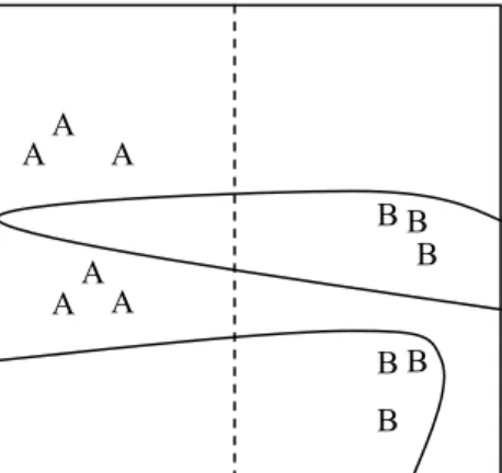
Most evaluation methods only take subset fit (or a version of subset fit where instances not present in the training set are also included) into consideration but the measure function proposed by [6] builds upon all three heuristics. There is often a trade-off between the three heuristics and the measure function reveals this trade-off. The measure function helps in analyzing the learned classifier and the partitioning of the decision space. For example, consider the two classifiers illustrated in fig. 1.
Both classifiers would get the highest score in a cross-validation test (since all instances are correctly classified by both classifiers). However, most people would regard the classifier making the simple division of the instance space using a straight line as better than the more complex one. A measure function would make it possible to capture this, e.g., by including simplicity and similarity as evaluation aspects.
A Multi-dimensional Measure Function for
Classifier Performance
Niklas Lavesson and Paul Davidsson SECOND IEEE INTERNATIONAL CONFERENCE ON INTELLIGENT SYSTEMS, JUNE 2004
Fig 1. The division of a two-dimensional instance space made by two different classifiers. One illustrated by the dashed line, and the other illustrated by the curves. The letters indicate the positions of the instances of the two categories (A and B).
Below, similarity and simplicity will be given a more detailed explanation. However, it is important to note that the concept of measure functions is not limited to the three heuristics discussed, but is a much more general concept where any aspect of the classifiers’ division of the instance space may be taken into account.
It is mentioned in the last chapter that similar instances should be classified similarly, but the question is how to define similar in this context. A classifier divides the instance space into several areas corresponding to different classes or categories, and we define a decision border as the border between two such areas. According to [6] one often used heuristic of similarity is that the decision borders should be centred between clusters of instances belonging to different classes. Thus in general terms, the distance between each instance and its closest decision border can be a measure of similarity.
The simplicity heuristic is used in order to reduce the chance of over-fitting the data. According to [6] simplicity is often measured with respect to a particular representation scheme. One example of measuring simplicity this way is to count the number of nodes in an induced decision tree. However, the measure function should be general enough to be applicable to any classifier independently on how it is represented and which learning algorithm was used to construct it. Thus, it should focus on the classifiers´ division of the instance space rather than on the classifiers themselves.
III.CROSS-VALIDATION EVALUATION
Cross-validation (CV) tests exist in a number of variants but the general idea is to divide the training data into a number of partitions or folds. The classifier is evaluated by its classification accuracy over one partition after having learned from the other. This procedure is then repeated until all partitions have been used for evaluation. Some of the most common types are 10-fold, n-fold and bootstrap CV [3]. The difference between these three types of CV lies in the way that data is partitioned. Leave-one-out is equal to n-fold CV, where n stands for the number of instances in the data set. Leave-one-out or n-fold CV is performed by leaving one instance out for testing and training on the other instances. This procedure is then performed until all instances have been left out once.
Bootstrap is based on sampling with replacement. The
data set is sampled n times to build a training set of n instances. Some instances will be picked more than one time and the instances that are never picked are used for testing. Even though CV tests can give a hint of how well a certain classifier will perform on new instances, it does not provide us with much analysis of the generalization capabilities and any analysis of the decision regions of the classifier. These and other bits of information extracted from a learned classifier may work as valuable clues when trying to understand how the classifier will perform on new instances. It has been argued that the design of 10-fold CV introduces a source of correlation since one uses examples for training in one trial and for testing in another [7].
IV.AMULTI-DIMENSIONAL MEASURE FUNCTION
The implementation discussed in this article builds upon the example measure function suggested by [6]. The main improvement is that the new version supports data sets with more than two attributes. In addition this version is integrated with WEKA, a popular machine learning environment, which makes it compatible with both the data set standard and the classifiers from that environment (this is further discussed in chapter IV). Since it is implemented in Java, the new version inherits the benefits of that language (e.g. platform independence and object-orientation). From now on we refer to the new implementation of the measure function as MDMF (Multi-Dimensional Measure Function) and to the Iris database [8], used for all experiments and examples in this article, as IRIS. In order to compute the similarity and the simplicity components, the instance space has been normalized. The instances of the data set are normalized by dividing their feature values by the highest found attribute value for each feature.
To measure similarity we need to calculate the distance,
d
, between each instance and its closest decision border. If an instance was correctly classified the similarity contribution of that instance is positive, otherwise it is negative. The reason for applying this rule is that correctly classified instances should preferably reside as far away as possible from the decision borders, as mentioned in the description of the similarity heuristic in chapter II. Incorrectly classified instances reside on the wrong side of the decision border so the contribution they make to similarity should be negative. Preferably these instances should reside close to the border of the correct class. This is implemented by letting the contribution be less negative if the instance is close to the correct class border. The formulas used to calculate the contribution ofd
to similarity are taken from the original measure function. The contribution from a correctly classified instance is 1 1/ 2− bd (1) and from an incorrectly classified instance 1/ 2bd−1 (2). The normalization constant,b
, for the similarity function is chosen in the same way as for the original measure function; the square root of the number of instances in the data set is used. Both (1) and (2) are functions with sigmoid-like behavior. They are asymptotically constant for large positive and negative values in order to capture the fact that instances very far from borders should not be affected by slight border adjusts. In order to find the A A B B A A A A B B B Bdecision border closest to an instance, we start from the location of the instance and search outwards. We cannot simply measure the length between an instance and a border in a trivial manner since it cannot be assumed that the classifier provides an explicit representation of the decision borders. By moving outwards in small steps and querying the classifier about the current position it is easy to determine if we have entered a region belonging to a different class than that of the instance. If this is the case a decision border has been found. The pseudo-code below shows the algorithm for computing the similarity.
Similarity(DataSet, Classifier) For Each Instance X in DataSet Prediction = Classifier.PredictClass(X) Class = DataSet.GetRealClass(X) Correct = (Class == Prediction) If (Not Correct) Class = Prediction SDist = 0
While (Class == Prediction) SDist += RadiusIncrease For Each Attribute Y in X
For Z=0 To Power(2, DataSet.NumAttr-1) Comb = ChooseCombination(Z) For Q = -SDist To SDist
Prediction = PredictNewPos(Comb, Q) Inc Q With ((SDist*2)/10)
If (Not Correct) ContributeDistNegative() Else ContributeDistPositive()
There are two functions that are not part of the pseudo-code and thus need to be explained further but first let us review the rest of the algorithm.
Each instance is classified and the result is compared with the correct class value. The search for a decision border starts at the position of the instance and the size of the search area is decided by SDist. SDist increases with RadiusIncrease (which is a configurable parameter of MDMF) for every search iteration. One search is conducted for each attribute and the search is organized as follows. First the ChooseCombination function is run: all attributes except the one to search are set to either a negative or a positive SDist value. The search attribute is set to a negative SDist value and then the PredictNewPos function is run: A prediction is made of the instance defined by the new attribute values. If the prediction differs from the earlier Prediction value we have found a decision border. If this is not the case, a new combination is chosen and the procedure is followed again. The distance between an instance and its closest decision border, d, is the Manhattan distance between the original instance position and the position of the instance defined by the current attribute values. Depending on the classification (Prediction was equal to Class or not) the contribution to similarity is computed with (1) or (2).
The computational effort needed to calculate similarity varies with the number of attributes per instance, the number of instances in the data set and the size of iterative search steps. The complexity of the similarity calculation is
( )
O nas where
n
is the number of instances,a
the number of attributes, ands
the number of possible search steps in each dimension.IRIS has four numerical attributes (and a nominal target attribute). To calculate similarity for a classifier learned
from this data set we have to search in four dimensions (one for each attribute) to locate the closest decision border for each instance. Actually, this is just an approximation since the closest border point may not be in one of these orthogonal lines. The data set consists of 150 instances so we need to perform 150 individual searches through all four dimensions to calculate the similarity aspect of MDMF. The step size is a parameter that can be decided by the user.
It has been suggested that simplicity can be measured by calculating the total size of the decision borders [6]. Unlike subset fit and similarity the simplicity value (the size of the decision borders) should be as low as possible. Although this is fairly simple to calculate in two or maybe even in three dimensions for classifiers that have explicit decision borders, it becomes increasingly hard to calculate for a larger number of dimensions, and for classifiers with implicit decision borders. The following way to approximate the decision border size was proposed by [6]: a number of lines are chosen each so that they cross the attribute space with a random direction and starting point. Decision border size is approximated as the average number of decision borders encountered when traveling along the lines. The procedure to find decision borders along a line is quite simple; at the start of the line the coordinates are used as attribute values for an instance and the learned classifier then classifies this instance and returns the predicted class. These events are then repeated at each step and if the class value returned has changed it means that we have found a decision border.
A problem with this way of measuring border size is the stochastic element: since random lines are chosen the result varies between runs and this should be avoided for stability and consistency reasons. Instead, we have implemented a deterministic simplicity calculation method. The results do not vary between runs simply because the stochastic elements have been removed from the solution. Simplicity is calculated by dividing the decision space into a grid and traveling along each grid line, querying the classifier for each position, in order to find out the average number of decision borders encountered. The size of the squares of the grid used for calculation of simplicity is changeable. Smaller size results in longer execution time but higher level of detail and vice versa. The complexity of the simplicity calculation is O g( )a where
g
is the number ofgrid squares per dimension and
a
is the number of attributes.TABLE I
MEASURE FUNCTION CONFIGURATION
Weight Affects Value
a0 Subset fit 1.0
a1 Similarity 1.0
a2 Simplicity 0.1
k1 Simi1 0.5
k2 Simi2 0.5
Detail Affects Value
square size Simplicity 0.0100 radius increase Similarity 0.0005
Default configuration of weights and level of detail for measure-based performance evaluation. Simi1 – Similarity of correctly classified instances, Simi2 – Similarity of incorrectly classified instances.
the original measure function: the learned classifier is evaluated using the training set and the subset fit measure result is calculated by dividing the number of correctly classified instances by the total number of instances. The complexity of the subset fit is
O n
( )
, wheren
is the number of instances.MDMF was implemented in Java using the WEKA machine learning workbench [3]. WEKA contains a collection of machine learning algorithms as well as tools for classification, visualization, regression and clustering. WEKA implementations exist for many of the well-known learning algorithms and these can be evaluated with MDMF. MDMF also makes use of the ARFF data set file format used by WEKA.
MDMF is very flexible and can be configured in many different ways, depending on the problem at hand. The different parts of the function are weighted in order to provide a way to focus on one or more specific aspects when evaluating and comparing classifier results. Subset fit, similarity and simplicity can all be weighted individually by changing variables a0, a and 1
a
2. Similarity is divided into two parts; similarity of correctly classified instances and similarity of incorrectly classified instances. These two parts of similarity can also be weighted differently and for this the variables k1 and k2 are used.0 1 1 1 2 2 2
a S u b setfit + a (k S im i + k S im i ) - a S im p (3) We can now describe the measure function as (3). Apart from tuning these weights, also the level of detail used for the simplicity and similarity calculations can be altered. Both simplicity and similarity are calculated by having the classifier query different points in the instance space in order to find out which class the point belongs to.
TABLE II DECISION TREE EVALUATION
Algorithm 10-CV MDMF
J48 0.953 1.086
J48-P 0.947 1.101
Pruned and unpruned decision trees evaluated with 10-fold cross-validation (10-CV) and measure function (MDMF).
Working with many data set attributes as well as large numbers of instances greatly increases the number of predictions that has to be made. As we learned from the complexity analysis of the similarity and simplicity computations, there is a trade-off between the level of detail and the execution time (as with most computational problems) and the balance depends on the specific problem to be solved. The MDMF configuration used in the example and the experiments of this article is detailed in table I.
Up till now we have presented the concept of measure-based evaluation and the implementation of the measure function. Let us demonstrate the functionality with an illustrative example. The WEKA implementation of C4.5 [9], which is called J48, is here used to induce two different decision trees from the IRIS data set. The first decision tree is left unpruned and reduced error pruning is applied on the second. The results are presented in table II.
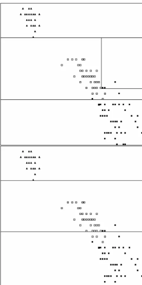
Fig. 2. Visualization of a two-dimensional decision space. An unpruned tree (top) and a pruned tree (bottom) have been produced by the J48 algorithm. Only two attributes of IRIS were used (petal width and height) in order to be able to visualize the decision space.
Table II shows that the two methods yield contradicting results. The unpruned decision tree obviously predicts with higher accuracy than the pruned tree in this example. The MDMF results can be explained by looking at table III.
TABLE III
MEASURE-BASED EVALUATION OF DECISION TREES
Algorithm Subset Similarity Simp MDMF
J48 0.980 0.756 2.724 1.086
J48-P 0.967 0.720 2.253 1.101
Subset – subset fit value, Simp – simplicity value, MDMF – resulting measure with the default configuration of MDMF.
In table III we can see that even though the accuracy is higher for the unpruned tree, the pruned version has a lower simplicity value indicating that it is a less complex, less over-fitted solution. Two-dimensional visualizations of the decision spaces of the two different decision trees can be seen in fig. 2. Intuitively the decision space of the pruned tree looks less over-fitted and less complicated.
What is important to notice here is the way the total measure gets calculated by combining the different parts along with their individual weights. After the evaluation has been performed the weights can be changed over and over again to reflect different views or perspectives of classifier performance. Different parts can be excluded by setting their corresponding weight to zero. The default configuration used in this article, discussed in chapter IV, is chosen so that each part contributes about equally to the resulting measure.
V.EXPERIMENTS
This section reviews two experiments conducted in order to demonstrate the usage of the new implementation. First
we describe an evaluation of classifiers learned by a number of commonly used learning algorithms. This is followed by execution time comparison.
Some of most common learning algorithms (each with a set of different configurations) have been used to produce classifiers and these classifiers have been evaluated using the default configuration of MDMF. See table IV for details.
TABLE IV
MEASURE-BASED EVALUATION OF COMMON CLASSIFIERS
Algorithm Subset fit Similarity Simp MDMF
J48 0.980 0.756 2.724 1.086 J48-p 0.967 0.720 2.253 1.101 IB1 1.000 0.692 4.300 0.916 IB10 0.967 0.717 3.762 0.949 BP2-500 0.987 0.720 4.196 0.927 BP2-5000 0.987 0.728 4.124 0.938 BP2-25000 0.987 0.723 3.935 0.955 BP3-20000 1.000 0.708 3.772 0.977 BP3-32000 1.000 0.707 3.778 0.976 NBayes 0.960 0.721 6.213 0.699
Evaluation of some of the most common classifiers, using the default configuration of the measure function.
Four different learning algorithms have been used to produce a set of classifiers for this evaluation experiment. The J48 algorithm, which we already have introduced in the example, has produced one pruned and one unpruned decision tree classifier. Both sub tree raising and reduced error pruning was applied on the first classifier. One of WEKA’s nearest neighbor implementations, called IBk, has been used to produce one classifier based on one neighbor (IB1) and another classifier based on ten neighbors (IB10). The back propagation (NeuralNetwork) algorithm has been used to produce five different neural network classifiers, each with a different combination of the number of hidden nodes (2 or 3) and the number of epochs for training.
The NaiveBayes algorithm has also been used to produce one classifier. Mitchell argues that this algorithm is known to perform comparably with decision tree and neural network learning in some domains [1]. This makes it an interesting algorithm to use in the experiments concerning the evaluation of classifiers using a measure function. Measure-based evaluation of the NaiveBayes classifier is compared with measure-based evaluation of decision trees and neural networks in order to find out if it performs comparably with them when measured with a multi-dimensional measure function instead of a CV test.
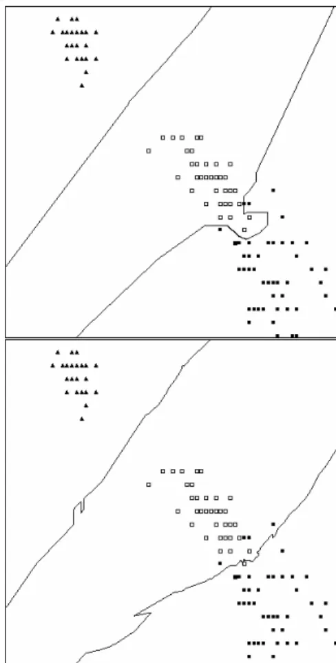
Let us first examine simplicity. It seems that the simplicity measure captured, quite well, the difference in decision space complexity between the pruned and unpruned decision tree. Fig. 2 shows this difference graphically (although only for two dimensions). The same pattern applies to the nearest neighbor classifiers. Fig. 3 shows the difference graphically between the decision spaces belonging to these two classifiers.
The Naive Bayesian classifier scored the highest (worst) simplicity value and the reason for that is easily interpreted by inspecting fig. 4.
If we look at the neural network classifier results we can see that the least complex classifier is the one produced with 3 nodes and with a training time of 20000 epochs.
Looking at the other node network with 3 nodes (trained for 32000 epochs) it seems to be a more over-fitted classifier, since both similarity and simplicity values are worse than that of the first classifier.
In the execution time experiment a number of classifiers were evaluated using two different configurations of the simplicity detail level property. Individual time measures are not important here, since they are tied to a very specific platform, but rather what is interesting is the difference in execution time for the different configurations and the difference in execution time when evaluating different classifiers.
Fig. 3. Visualization of a two-dimensional decision space. IB with 1 neighbor (top) and IB with 10 neighbors (bottom) have been produced by the IBk algorithm.
Fig. 4. Visualization of a two-dimensional decision space. A classifier produced by the NaiveBayes algorithm.
The correlation coefficient is 0.99 when calculated from the two different time measures in table V. We can therefore assume that the increase in execution is only related to the level of detail and not to which classifier is evaluated. It is easy to notice that the nearest neighbor
classifiers take by far the longest time to evaluate. This is attributed to the fact that the instance-based algorithms are lazy learners.
They learn quickly, by just storing the instance to be learned, but because of this they have a tendency to be slow at classification. In order to compute similarity and simplicity a large number of classifications must be executed, thus a slow classifier results in a slow evaluation.
The classifier need to be produced once prior to the evaluation when using MDMF, which means a slow learner does not affect the evaluation time much. This could be compared with 10-fold CV, for which the classifier must be produced 10 times, once for each fold, to compute the test score. Consequently the reverse situation holds for CV tests: a slow learner has a more negative affect on the evaluation time than a slow classifier. For example, back propagation is evaluated very slowly with CV, but instance-based algorithms are evaluated quickly.
TABLE V
TIME CONSUMED BY EVALUATION
Algorithm 10 grid 100 grid
J48 19 ms 337 ms J48-P 18 ms 368 ms 1-NN 1738 ms 25905 ms 10-NN 2103 ms 27501 ms BP2-500 56 ms 849 ms BP2-5000 58 ms 851 ms BP3-20000 69 ms 936 ms BP3-32000 64 ms 950 ms NBayes 83 ms 1148 ms
The time for evaluating some common classifiers using a) a simplicity level of detail of 10 grid squares per dimension, and b) a simplicity level of detail of 100 grid squares per dimension.
VI.CONCLUSIONS AND FUTURE WORK
Although Cross-validation tests are the most frequently used method for classifier performance evaluation, we argue that it is important to consider that it only take accuracy into account. We have shown, with a theoretical example in chapter II as well as in a practical experiment in chapter IV, that measure functions may reveal aspects of classifier performance not captured by evaluation methods based solely on accuracy. By altering the weights or changing the level of detail the measure function evaluation can be biased towards different aspects of classifier performance, useful for a specific class of problems. The new measure function presented in this article, MDMF, supports evaluation of data sets with more than 2 attributes, making it useful for a larger amount of evaluation problems than the original measure function example. It is however important to note that the concept of measure functions is not limited to the three heuristics discussed in this article. Thus, the implementation could be further expanded with more heuristics in the future. An important issue for future study is methods for determining the appropriate weights for a given domain (data set).
Currently, MDMF only supports normalized data sets with numerical features and a nominal target attribute. This means that it can only evaluate classifiers learned from one specific type of data set. Although this type probably is the most common, it would be interesting to extend the
capabilities of the measure function so that it can manage evaluations of also other types of data sets containing, e.g., Boolean and nominal features.
The method used to calculate simplicity in MDMF is very different from that of the original measure function, in which the total length of the decision borders was used as a simplicity measure. Since the new implementation supports n dimensions it is not possible to measure the decision border lengths (at least not for dimensions higher than 2). As a result another measure for simplicity has been used; the average number of decision borders encountered when traveling through decision space in any direction. Experiments have shown that this measure captures the difference between pruned and unpruned decision trees but there may be other measures of simplicity that are less complex and have even better qualities.
The measure function, as an evaluation method, could be combined with optimization methods such as genetic algorithms and simulated annealing to produce optimal classifiers given a specific class of problems. Simpler version of this approach has been done by using accuracy measures as fitness functions or thresholds [10], [11].
We plan to develop a public web site that demonstrates the functionality and benefits of the multi-dimensional measure function. Users will be able to interactively supply data, choose a learning algorithm and configure both the algorithm and the measure function. The user would then have the possibility to view the resulting measure with the present configuration or change the different weights and see the changes in realtime.
REFERENCES
[1] T. M. Mitchell, Machine Learning, International Edition, McGraw-Hill Book Co, Singapore, ISBN: 0-07-042807-7, 1997.
[2] N. M. Adams and D. J. Hand, Improving the practice of classifier performance assessment, Neural Computation, vol.: 12 issue: 2, MIT press, pp. 305-312, 2000.
[3] I. H. Witten and E. Frank, Data Mining: Practical machine learning
tools and techniques with Java implementations, Academic press,
Morgan Kaufmann publishers, ISBN: 1-55860-552-5, 1999. [4] G. Bebis and M. Georgiopoulos, “Improving generalization by using
genetic algorithms to determine the neural network size”, Southcon
95, Fort Lauderdale, Florida, pp. 392-397, 1995.
[5] A. Andersson, P. Davidsson and J. Lindén, Measuring generalization quality, Technical report LU-CS-TR: 98-202. Department of Computer Science, Lund University, Lund, Sweden, 1998.
[6] A. Andersson, P. Davidsson and J. Lindén, Measure-based classifier performance evaluation, Pattern Recognition Letters, vol.: 20 issue: 11-13, North-Holland, Elsevier, pp. 1165-1173, 1999.
[7] M.A. Maloof, “On machine learning, ROC analysis, and statistical tests of significance”, 16th International Conference on Pattern
Recognition, IEEE, vol.: 2, pp. 204-207, 2002.
[8] E. Anderson, The irises of the Gaspe peninsula, Bulletin of the
American Iris society, vol.: 59, pp. 2-5, 1935.
[9] J. Quinlan, Programs for Machine Learning, Morgan Kaufmann, San Francisco, ISBN: 1-55860-238-0, 1993.
[10] S.-Y. Ho, C.-C. Liu and S. Liu, Design of an optimal nearest neighbor classifier using an intelligent genetic algorithm, Pattern
Recognition Letters, vol.: 23 issue: 13, North-Holland, Elsevier, pp.
1495-1503, 2002.
[11] S. Chalup and F. Maire, “A study on hill climbing algorithms for neural network training”, 1999 Congress on Evolutionary