Optimization importance in high-frequency algorithmic trading

(1)

Optimization importance in high-frequency

algorithmic trading

Vadim Suvorin

Dmytro Sheludchenko

(2)

The thesis offers a framework for trading algorithm optimization and tests statistical and economical significance of its performance on American, Swedish and Russian fu-tures markets. The results provide strong support for the proposed method, as using the presented ideas one can build an intraday trading algorithm that outperforms the market in long term. Section 1 formulates the problem and reviews previous investigations in the area. Section 2 describes the data, trading algorithms, their optimization framework and testing methodology. Section 3 presents the empirical results of proposed framework implementation, compares its performance with random parameters trading and market buy-and-hold profit.

(4)

1 Introduction

Trading strategies have existed ever since first capital markets emerged, as every market participant follows some sort of trading rules. Ability of a trading algorithm to generate ex-cess return has always been closely connected to the Efficient Markets Hypothesis (EMH), which was independently proposed by Eugene Fama and Paul Samuelson in 1965. According to EMH, the market is efficient when prices of traded instruments fully reflect all available information. This theory is one of the most controversial in finance and has provoked many heated discussion between its supporters and challengers.

EMH theory suggests that there is no point in trying to identify mispriced securities or to utilize different analysis techniques to predict future price movements. As it was pointed out by Shostak (1997), EMH implies that the simplest buy-and-hold strategy is as profitable as any other and that there is no place for entrepreneurial activity in financial markets [8].

One of the biggest EMH supporters, Malkiel from Princeton University, claimed in 1973 that a blind-folded chimpanzee throwing darts at the Wall Street Journal could be as success-ful at selecting stocks as portfolio managers and stock analysts with many years of market experience and training [5].

The first tests of EMH were aimed at proving its weak efficiency, which implies that current stock prices fully reflect the information about historical prices. This question is thoroughly investigated in Fama’s working papers in 1965 and 1970 that revolved around measuring the serial correlation of stock market returns [4].

Similar studies were later performed by Conrad, Kaul, Lo and MacKinlay in 1988. They analyzed returns of NYSE stocks on per-week basis and found positive serial correlations over short time periods. However, the correlations were rather low, especially for large-cap stocks. Due to this fact, the respective authors could not prove existence of opportunities to earn excessive returns despite proving existence of short term trends.

The study by Jegadeesh and Titman (1993) pointed out ”momentum effect” in stock per-formance that continued over time. They compared two different stock portfolios: one con-sisting of best performing stocks in the past, while the other contained stocks that performed badly. They proved that the portfolio of best-performing stocks led to higher returns in the fu-ture, thus creating profit opportunities for investors. This fact is considered to prove short-term price momentum and undermine EMH.

Papers by Fama and French (1988) and Poterba and Summers (1988) found existence of prolong negative long-term serial correlation of the aggregate market, which implied market’s overreaction to particular news in one time period. This effect led to positive correlation over short-term horizon and eventual correction in following time period.

The first studies that investigated the ability of technical analysis to boost returns were conducted by Fama and Blume in 1966 and Jensen and Benington in 1970 and concluded that technical algorithms did not lead to increased returns. This result was not questioned for more than two decades. The study by Brock, Lakonishok and LeBaron published in 1992 changed this perception [1]. The authors investigated two very popular trading strategies, moving average and trading-range breaks, on a huge data sample of Dow Jones Average Index from 1897 to 1986 and concluded that even the simplest trading strategies had predictive

(5)

power and led to increase in returns. The researchers also proved that popular fitted time series models (random walk with a drift, AR, GARCH-M and EGARCH) could not explain the returns, generated by the trading strategies [2].

Similar results were obtained by Bessembinder and Chan in 1997. The authors examined returns of DJIA on four sub-periods from 1926 to 1991 and came to results, which support the previous study by Brock et al. However, they also suggested that high transaction costs could dismiss abnormal returns provided by market timing and lead to returns lower than market [1]. More modern studies, such as Holzmann and Reschenhofer (2010), confirm findings of Brock, Bessembinder and Chan, and also suggest that transaction costs are much lower nowadays and many brokers offer flat transaction rate, which is especially advantageous for high-frequency trading systems [7].

Despite a lot of studies concluded that algorithmic trading could outperform the market, there are not many works that investigate if historical performance of strategies is represent-ative. The latter is becoming a dominant issue as trading strategies’ complexity evolves on day-to-day basis and many practitioners, facing the challenge of choosing right trading rules with adequate parameters, base their decisions on backtesting results.

Although it’s obvious that history doesn’t always repeat itself on financial markets, some results from the business world suggest a positive effect of historical optimization on perform-ance of algorithmic trading strategy. One of numerous examples is XT-99, the algorithmic trading program that has generated average yearly return of 27,17% during time period between 1999 and 2011, while the average yearly return of S&P500 for the mentioned time period was 3,3% and return of Altegris 40 Index, which compiles 40 best returns from 500 CTA trading programs, was 6,56% [6].

The purpose of this paper is to determine if a trading strategy benefits from properly de-signed optimization. To achieve the purpose we test the hypothesis: historical optimization is able to improve out-of-sample performance of an algorithm.

The remainder of the thesis is organized as follows: Section 2 describes the data, trading strategies under consideration and optimization methodology; Section 3 presents the empir-ical results of proposed framework implementation, compares its performance with random parameters trading and the market; Section 4 concludes and summarizes our results.

(6)

2 Data and methodology

2.1 Data

In this study we focus on futures contracts, as transaction costs on this market are low enough to implement high-frequency trading ideas. We have chosen three markets with its most liquid instruments: E-mini S&P 500, OMXS30 and RTS index contracts, traded on CME, NASDAQ OMX and RTS Forts respectively. The sample contains minute timeframes from 15 Dec 2005 till 15 Feb 2012, which is equal to approximately 600 thousand returns for each market. The start date is chosen in such a way that volumes suffice for trading on minute timeframes. American market had enough liquidity even before the chosen date, but we decided to have the equal size of sample for all three instruments in order to facilitate the performance comparison. Due to lack of trading volumes, the night session was excluded from E-mini S&P 500 time series as well as the evening session on Russian market.

2.2 Trading strategy definition

In order to proceed, we should give a proper definition to a term trading strategy. It can be defined as a predetermined set of rules that one applies while making trading decisions [6]. In other words, it is an algorithm that one employs to filter out possibly predictive periods from non-predictive periods in time series. To give a mathematical definition, we must introduce the following notations:

O_t= open price for period t Ht= highest price for period t

Lt= lowest price for period t

C_t= closing price for period t

V_t= number of contracts traded in period t r_t=Ct/Ct−1− 1 = market return for period t

The processes above comprise a sequence of market information flow for technical trad-ing system. Then a tradtrad-ing strategy will be a function φ with parameters ψ, which maps information available up to moment (t-1) to trading signals (χ_{t,φ ,ψ}) (unique for every strategy) and stop loss/ take profit prices both for long positions (SL_{t,φ ,ψ}ˆ ,T P_{t,φ ,ψ}ˆ ) and short positions (SL_{t,φ ,ψ}ˇ ,T P_{t,φ ,ψ}ˇ ):       ˆ SL_{t,φ ,ψ} ˆ T P_{t,φ ,ψ} ˇ SL_{t,φ ,ψ} ˇ T P_{t,φ ,ψ} χt,φ ,ψ       = φ (ψ, Oi, Hi, Li,Ci,Vi), i= 1, 2, . . . ,t − 1

Based on trading signals χ we can define a setA_{φ ,ψ}ˆ that contains periods, during which a strategy φ with parameters ψ stays in long position, and a setA_{φ ,ψ}ˇ that contains corresponding

(7)

periods for short positions. To determine when a position is closed by stop loss or take profit we introduce following sets:

ˆ B_{φ ,ψ} = ˆA_{φ ,ψ}∩ {t : Ht≥T Pt,φ ,ψˆ } ˆ C_{φ ,ψ} = ˆA_{φ ,ψ}∩ {t : Lt ≤SLt,φ ,ψˆ } ˇ B_{φ ,ψ} = ˇA_{φ ,ψ}∩ {t : Lt ≤T Pt,φ ,ψˇ } ˇ C_{φ ,ψ} = ˇA_{φ ,ψ}∩ {t : Ht≥SLt,φ ,ψˇ }

Returns process for long positions of strategy φ with input parameters ψ will be: ˆ

r_{t,φ ,ψ} = rt1A\(B∪C)+ T Pt/Ct−11B\C+ SLt/Ct−11C

where T Pt =T Pt,φ ,ψˆ , SLt =SLt,φ ,ψˆ , A =Aφ ,ψˆ , B =Bφ ,ψˆ , C =Cφ ,ψˆ and 1A(t) denotes an

indicator function:

1A(t) =

(

1,t ∈ A 0,t /∈ A

For short positions process of strategy returns is built by analogy: ˇ

r_{t,φ ,ψ} = −r_t1_A\(B∪C)− T P_t/C_t−11_B\C− SL_t/C_t−11C

where T Pt=T Pt,φ ,ψˇ , SLt =SLt,φ ,ψˇ , A =Aφ ,ψˇ , B =Bφ ,ψˇ , C =Cφ ,ψˇ

Out of the described processes we obtain strategy returns r_{t,φ ,ψ}= (r_{t,φ ,ψ}ˇ +r_{t,φ ,ψ}ˆ )/2, which can be easily transformed to value process for our trading portfolio:

V(T ) = V (0)

T

∏

t=1

(r_{t,φ ,ψ}+ 1)

where t = 1, 2, . . . , T are rebalancing points for individual strategy [3].

In this paper we look closely at five different trading algorithms: Moving average, Relative Strength Index, Tweezer, Trading Range Break and Momentum. In order to obtain a repres-entative estimate of optimization applicability, the strategies were chosen in such fashion that they work completely different.

2.2.1 Moving Average

This is a classical technical analysis trading strategy, which employs two moving aver-ages of different time periods in order to find a trend’s direction. The buying opportunity occurs when the fast moving average goes above the slow moving average (the trend seems to become bullish). The trading strategy is set to open a short position when the fast moving average intersects the slow moving average from above. In our tests, we use this strategy in the canonical way described above. No stop loss or take profit is involved, which means that strategy is always in position. As we see from Figure 1, position is open on the next bar after moving averages cross.

(8)

Figure 1: Moving Average trade example. Optimization parameters:

ψ1= 10, 15, . . . , 60 = length of fast moving average1;

ψ2= 2, 3, . . . , 6 = ratio of slow moving average length to length of fast moving average.

2.2.2 Relative Strength Index

The Relative Strength Index strategy is also very popular among traders. It measures the current and historical strength or weakness of an instrument.

The trading strategy takes long position when RSI value crosses up a lower barrier (ψ1)

and closes it when the indicator reaches middle level 50. Short position is opened, when stock price is considered overbought but starts to move back to regular levels, e.g. when the indicator crosses below a higher barrier (100-ψ1).

Stop loss for long position is put ψ3 minimum price changes lower than the lowest price

of the signal bar. For short position stop loss is placed ψ3 ticks higher than its highest price.

Full trade example is depicted in Figure 2.

Figure 2: Relative Strength Index short trade example.

(9)

Optimization parameters:

ψ1= 15, 18, . . . , 42 = lower barrier;

ψ2= 10, 12, . . . , 20 = length of the indicator;

ψ3= 1, 2, . . . , 5 = distance between high/low and stop loss price in minimum price changes.

2.2.3 Tweezer

Tweezer belongs to the family of candlestick strategies. The long position is opened after the specific pattern Bullish Tweezer, which is defined as a black candle, followed by a white candle with the same low level. Stop loss is placed on the lowest price of the candlestick formation with an indent of ψ1ticks. Take profit is put ψ2 minimum price changes from the

price of position opening. The short sale is performed by analogy after Bearish Tweezer.

Figure 3: Tweezer short trade example. Optimization parameters:

ψ1= 1, 3, 5 = distance between high/low and stop loss price in ticks.

ψ2= 12, 16, . . . , 80 = the value of take profit in minimum price changes.

2.2.4 Trading Range Break

With this rule signals are generated when the price moves above or below predefined sup-port and resistance level(this strategy is also known as Supsup-port/Resistance strategy). Supsup-port level is constructed upon the minimum of four last down fractals. Resistance level is based on four last up fractals2. Stop loss for long trades is placed ψ1minimum price changes lower

than former resistance level. Take profit is calculated according to ψ2.

2_{Up fractal is a candlestick pattern, which has its highest high in the middle and two lower highs on the sides}

of formation. Down fractal also contains five candlesticks with lowest low in the middle and two higher low on the sides.

(10)

Figure 4: Trading Range Break trade example. Optimization parameters:

ψ1= 1, 2, . . . , 5 = distance between support/resistance level and stop loss price in ticks.

ψ2= 5, 6, . . . , 30 = the value of take profit in minimum price changes.

2.2.5 Momentum

This strategy is mainly aimed to obtain quick profits on rapid market swings. The main focus is to catch movement of price in one direction on high volume. As soon as a trader notices acceleration in stock price or trading volume the trader will either buy or short sell in hope that the impulse is going to have a positive response. To identify the impulse average market return and average trading volume are calculated for the last 30 time periods.

r_t = |rt−30| + . . . + |rt−1| 30

V_t =Vt−30+ . . . +Vt−1 30

Long position is taken when rt/rt ≥ ψ1and Vt/Vt≥ ψ2.

Short selling is initialized when −rt/rt ≥ ψ1 and Vt/Vt ≥ ψ2. Positions are held for 10

time intervals.

Optimization parameters:

ψ1= 2, 3, 4, 5 = current return to the average value ratio, sufficient to open a position

ψ2= 2, 3, 4 = current volume to the average value ratio, sufficient to open a position

2.3 Optimization framework

As it was mentioned before, the purpose of optimization is to choose right strategy with ad-equate parameters from a myriad of different trading techniques. We base our choice solely on in-sample performance of trading algorithm, however there’re several nuances of optimization procedure that are worth mentioning.

To avoid overfitting, we introduce the following requirements for the optimization sample: • statistical representativeness, which implies contents of market movements of different direction and amplitude (uptrends, downtrends, flat market, periods of both high and low volatility);

(11)

• sufficient length that leaves more than 99% of degrees of freedom after exclusion of data points, consumed by optimization parameters and trading rules.

The optimization method we use is the grid search, which calculates and ranks every histor-ical simulation specified. Only key parameters that have a significant impact on performance are optimized. The range of every parameter is chosen subjectively in such a way that even minimum and maximum values are common-sense and tradable. The optimization step is set to be minimal after consideration of computational speed.

To build objective function we use three factors: • return over the sample;

• maximum drawdown of capital in percentage; • correlation with the market.

The exact forms of objective functions are given in Section 3.

The open size is equal to one contract and position is always closed on the last bar of a trading day. Realistic transaction costs are incorporated in every trade.

After historical simulations a performance of every unique set of parameters is measured and an optimal ψ∗ is determined as the one that maximizes the objective function. Then we compare optimized strategies with each other and form a trading portfolio of several al-gorithms.

2.4 Testing methodology

For in-sample performance cannot be a representative estimate of real results, we construct so called rolling optimization with walk forward analysis. It implies that the trading rules are determined in-sample, following the framework from Section 2.3, but tested out-of-sample. Then both periods are shifted forward and optimization with consequent walk-forward tests are repeated. In order to implement this framework we divide the full sample into subsamples of equal size τ.

Final return of trading algorithm φ with parameters ψ over subsample i is denoted by:

R_{i,φ ,ψ} =

τ i

∏

t=1+τ(i−1)

(r_{t,φ ,ψ}+ 1) − 1, i= [1; N]

The final return over the full sample is:

R_{φ ,ψ} =

N

∏

i=1

(R_{i,φ ,ψ}+ 1) − 1

The length of subsample τ is chosen in such a way that every interval corresponds to previously specified requirements. This can be achieved by inclusion of approximately 80000 intraday returns in each subsample. Even the most data consuming strategy Moving Average Intersection with maximum length of indicators requires only 360 input points, which deprives us of approximately 0.45% of freedom.

(12)

To test statistical significance we use bootstrapping methodology, as it’s unrealistic to draw any assumptions about returns distribution [2]. To determine if optimization is helpful for a strategy φ we randomly choose parameters before each subsample and evaluate P(R > R∗) as a portion of randomly obtained returns that outperform the chosen optimal ψ∗ out-of-sample. Parameters are chosen from the predefined set that is used for optimization. Number of simulations is equal to 100 000. Null-hypothesis about randomness of achieved result is rejected, when p-value falls under specified significance level.

The framework performance is tested by analogy, but random strategies with random para-meters are taken to trade forward.

Final results are compared with the market performance to reason economical significance of the optimization algorithm.

(13)

3 Empirical results

In this section we implement the proposed framework to find out the set of optimal para-meters ψ∗ for each algorithm and calculate weights of strategies upon the results of optimiz-ation. Hereupon we perform walk-forward analysis and compare the final performance with random parameters trading and buy-and-hold market result.

3.1 Optimizing the algorithm

First we optimize each algorithm and check if it gives us significantly better results than trading the strategy with random parameters. To find ψ_i∗ we employ four different objective functions.

At first, we ignore the question of risk and assume that we can maximize strategy out-of-sample performance by taking the set of parameters that has given us the highest return over subsample. Therefore we use ψ_i∗ that solves max_ψ(Ri−1,φ ,ψ). The walk-forward results of

using return as an assessment criterion are given in Table 1.

Table 1: Walk-forward results for the Highest Return Optimization

φ E-mini S&P 500 OMXS30 Futures RTS Futures

R p-val R p-val R p-val

Tweezer −47.42% 2.68% 69.99% 5.42% 71.52% 4.78%

MA 61.30% 13.82% 56.35% 73.06% 31.29% 86.51%

RSI −11.55% 13.77% 114.96% 0.00% 373.25% 0.00%

Support/resistance −55.47% 0.21% 27.33% 64.57% 93.82% 0.03%

Market Impulse −7.23% 8.19% 6.26% 40.36% 23.97% 27.60%

Optimization with Highest Return objective function clearly gives us substantial excess performance over random parameters trading for Tweezer and Relative Strenght Index. Ob-tained p-values are lower than 10% significance level or close to it, pointing out that these returns are not achieved by chance. The results of the other strategies are controversial. Op-timization of Moving Average and Market Impulse shows some considerable improvement over trading with random parameters only on the American market. Support/Resistance ex-cess return is statistically significant on the American and Russian markets, but negligible while trading Swedish OMXS30 futures.

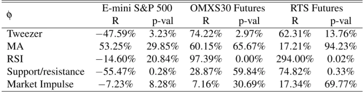
As a second criterion we use Reward to Risk Ratio, which interprets risk as a maximum drawdown of capital:

RRR_{i,φ ,ψ} = (

R_{i,φ ,ψ}/DD_{i,φ ,ψ}, if R_{i,φ ,ψ} ≥ 0 R_{i,φ ,ψ}DD_{i,φ ,ψ}, if R_{i,φ ,ψ} < 0

(14)

Table 2: Walk-forward results for the Highest RRR Optimization

Tweezer −47.59% 3.23% 74.22% 2.97% 62.31% 13.76%

MA 53.25% 29.85% 60.15% 65.67% 17.21% 94.23%

RSI −14.60% 20.84% 97.39% 0.00% 294.00% 0.02%

Market Impulse −7.23% 8.28% 7.16% 30.69% 17.34% 69.77%

After incorporation of risk in objective function, the returns of some trading strategies visibly decline. The corresponding p-values for Moving Average and RSI on the American market are no longer close to critical area, making these returns statistically insignificant. The rest of strategies perform almost the same as with the Highest Return optimization.

Designing the consecutive evaluation criteria we take into consideration the dependence on the market β , which is estimated as correlation between market and strategy returns within subsample. The combination of profitability and market dependence gives us two following indicators, which basically differ only in weights of described factors.

ζi,φ ,ψ =

(

R_{i,φ ,ψ} / |βi,φ ,ψ|, if Ri,φ ,ψ ≥ 0

R_{i,φ ,ψ} |βi,φ ,ψ|, if Ri,φ ,ψ < 0

ζ_{i,φ ,ψ}0 = (

R_{i,φ ,ψ} /p|β_{i,φ ,ψ}|, if Ri,φ ,ψ ≥ 0

R_{i,φ ,ψ} p|β_{i,φ ,ψ}|, if Ri,φ ,ψ < 0

β_{i,φ ,ψ} = Cor(rt, rt,φ ,ψ), t= 1 + τ(i − 1) . . . τi

Corresponding results are displayed in Tables 3 and 4.

Table 3: Walk-forward results for the Highest ζ Optimization

Tweezer −60.17% 92.67% 27.61% 92.69% 59.87% 18.04%

MA 44.76% 50.21% 57.48% 72.03% 170.09% 11.45%

RSI −23.88% 53.92% 36.94% 5.68% 217.59% 0.62%

(15)

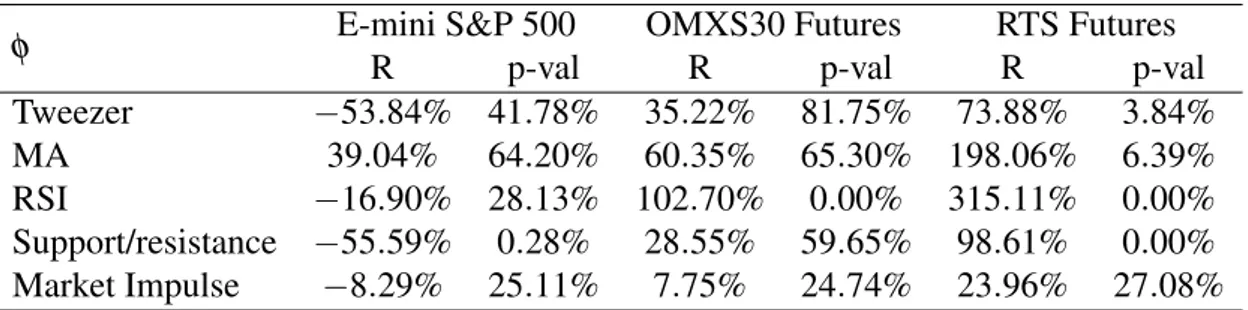
Table 4: Walk-forward results for the Highest ζ0Optimization

Tweezer −53.84% 41.78% 35.22% 81.75% 73.88% 3.84%

MA 39.04% 64.20% 60.35% 65.30% 198.06% 6.39%

RSI −16.90% 28.13% 102.70% 0.00% 315.11% 0.00%

Market Impulse −8.29% 25.11% 7.75% 24.74% 23.96% 27.08%

Incorporation of the market correlation considerably worsens out-of-sample return of all strategies. The only exception is Moving Average on the Russian market, whose perform-ance soars after taking β into account. Lowering the weight of β in the evaluation criterion increases the returns inessentially (Table 4). As an improvement over the Highest Return op-timization takes place only in one case on one market, we exclude ζ and ζ0 from the list of performance indicators while comparing the algorithms with each other.

To sum up, maximization of in-sample final return has a significant positive impact on out-of-sample performance of Tweezer and Relative Strength Index. Optimization of Moving Average, Support/Resistance levels and Market Impulse also gives significantly better results than trading with random parameters, but not on all the markets. Incorporation of capital drawdown in the objective function exerts a negative influence on performance in general, but the most of algorithms maintain the returns on the same level. Correlation with the market is not relevant to evaluate strategy performance.

3.2 Choosing the strategy

Next step after parameters optimization is choosing the strategy to trade forward. Fol-lowing the rules of diversification, it seems reasonable to include more than one algorithm in trading portfolio, therefore we divide invested capital into several parts. By analogy with optimization of parameters, the weights are based solely on in-sample performance, which represents a degree of strategy credibility. Performance is assessed with the help of two indic-ators: Return over the subsample and Reward to Risk Ratio.

We also introduce barriers and don’t trade forward the strategy if its best return is neg-ative in optimization subsample or maximum RRR is less than one. Weight of strategy φ in subsample i is calculated as following:

ω_i,φ = (R∗_i−1,φ)+/

∑

φ (R∗_i−1,φ)+ ω_i,φ0 = (RRR∗_i−1,φ− 1)+/

_∑

φ (RRR∗_i−1,φ− 1)+ R∗_i−1,φ = max ψ (Ri−1,φ ,ψ), RRR∗_i−1,φ = max ψ (RRRi−1,φ ,ψ), (x)+≡ max(x, 0)

(16)

3.3 Walk forward results

Walk forward results for the American market are displayed in Tables 5 and 6. We also calculate p-values for final returns over the full sample by simulating the trading of random strategy with random parameters.

Table 5: E-mini S&P 500. Walk forward results for the Highest Return optimization.

Subsample Portfolio Market

R DD RRR R DD RRR 2 0.11% 4.63% 0.02 6.67% 12.23% 0.55 3 5.94% 5.23% 1.14 −16.49% 22.73% 0.00 4 25.22% 8.45% 2.99 −25.84% 49.18% 0.00 5 2.44% 3.99% 0.61 25.51% 9.47% 2.69 6 4.41% 3.57% 1.21 10.60% 17.2% 0.62 7 5.82% 3.20% 1.82 5.28% 19.68% 0.27 Final 50.16% 8.45% 5.94 −3.42% 57.94% 0.00

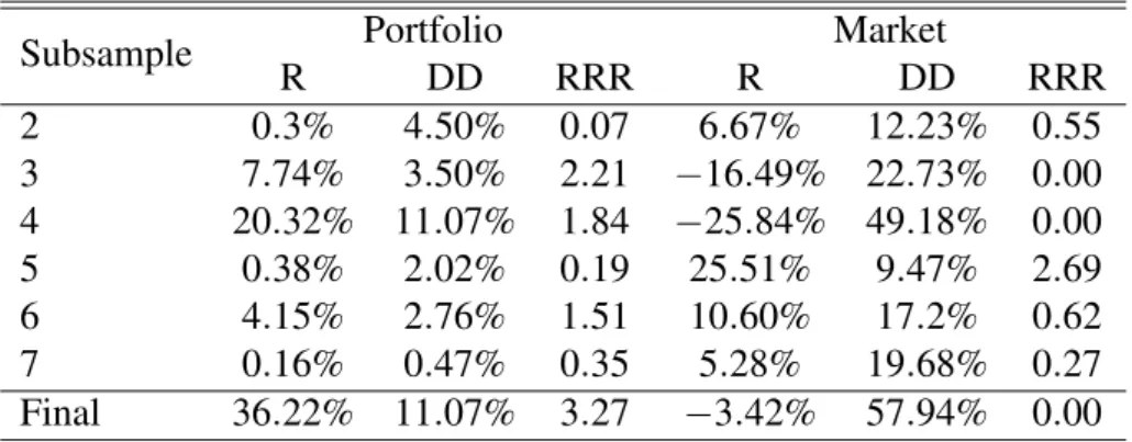
Table 6: E-mini S&P 500. Walk forward results for the Highest RRR optimization.

R DD RRR R DD RRR 2 0.3% 4.50% 0.07 6.67% 12.23% 0.55 3 7.74% 3.50% 2.21 −16.49% 22.73% 0.00 4 20.32% 11.07% 1.84 −25.84% 49.18% 0.00 5 0.38% 2.02% 0.19 25.51% 9.47% 2.69 6 4.15% 2.76% 1.51 10.60% 17.2% 0.62 7 0.16% 0.47% 0.35 5.28% 19.68% 0.27 Final 36.22% 11.07% 3.27 −3.42% 57.94% 0.00

P-values for returns of both strategy portfolios are less than 0.01%, which suggests that both optimization frameworks result in statistically significant improvement over random parameters trading. The Highest Return objective function helps to outperform the market in 4 of 6 subsamples and results in substantial performance improvement over the full sample. The Highest RRR objective function gives better results than the market in 3 of 6 cases and maintains outperformance of the overall return, though slightly decreasing the returns.

(17)

Table 7: OMXS30 futures. Walk forward results for the Highest Return optimization.

R DD RRR R DD RRR 2 11.6 − % 4.62% 2.51 −13.5% 31.50% 0.00 3 18.14% 6.82% 2.66 −34.06% 45.21% 0.00 4 8.73% 3.51% 2.49 44.45% 10.29% 4.32 5 4.45% 3.28% 1.36 15.10% 13.04% 1.16 6 12.43% 3.71% 3.35 −15.71% 29.46% 0.00 Final 68.35% 6.82% 10.02 −20.06% 57.94% 0.00

Table 8: OMXS30 futures. Walk forward results for the Highest RRR optimization.

R DD RRR R DD RRR 2 11.69% 3.51% 3.33 −13.5% 31.50% 0.00 3 21.54% 5.27% 4.09 −34.06% 45.21% 0.00 4 6.94% 4.13% 1.68 44.45% 10.29% 4.32 5 5.84% 2.79% 2.10 15.10% 13.04% 1.16 6 9.88% 3.16% 3.13 −15.71% 29.46% 0.00 Final 68.85% 5.27% 13.06 −20.06% 57.94% 0.00

The Swedish market (Tables 7 and 8) is outperformed in 3 of 5 cases by both objective functions. Corresponding p-values are 2.28% and 2.02%. The overall excess return, given by the algorithm is almost 90%, which is three times higher than one obtained on the American market. The latter supports the statement of less efficiency of NASDAQ OMX Nordic, as information on less efficient markets is absorbed slower giving additional opportunities for traders.

Table 9: RTS futures. Walk forward results for the Highest Return optimization.

R DD RRR R DD RRR 2 10.43% 5.96% 1.75 −1.79% 23.76% 0.00 3 36.58% 13.19% 2.77 −70.46% 78.26% 0.00 4 23.92% 6.51% 3.68 128.64% 36.11% 3.56 5 3.05% 6.88% 0.44 −8.46% 26.99% 0.00 6 7.06% 2.94% 2.41 33.78% 12.93% 2.61 7 5.50% 3.04% 1.81 10.88% 16.70% 0.65 8 11.19% 5.40% 2.07 −16.79% 41.43% 0.00 Final 141.86% 13.19% 10.76 −25.17% 81.34% 0.00

(18)

Table 10: RTS futures. Walk forward results for the Highest RRR optimization.

R DD RRR R DD RRR 2 13.42% 3.84% 3.49 −1.79% 23.76% 0.00 3 33.43% 10.00% 3.34 −70.46% 78.26% 0.00 4 21.37% 6.21% 3.44 128.64% 36.11% 3.56 5 7.35% 2.88% 2.55 −8.46% 26.99% 0.00 6 6.56% 1.79% 3.67 33.78% 12.93% 2.61 7 7.25% 1.87% 3.88 10.88% 16.70% 0.65 8 9.61% 2.70% 3.43 −16.79% 41.43% 0.00 Final 147.01% 10.00% 14.7 −25.17% 81.34% 0.00

The Russian futures market (Tables 9 and 10) is outplayed in 4 of 6 cases, giving the overall surplus return of 170%. These results are consistent with the notion that the Russian market is thought to be less efficient than Swedish or American. P-values are 6.05% for the Highest Return optimization and 5.43% for the Highest RRR.

The other important detail is the drawdown over the full sample. The first objective func-tion has given us 9% versus 58% on the American market, 7% versus 58% on the Swedish market and 13% versus 81% on the Russian market. The maximization of RRR has achieved the level of risk to 11%, 5% and 10% for corresponding markets.

Upon the simulation results we can conclude that on all markets under investigation the optimization helped to attain a significant outperformance both in return and risk level.

4 Conclusion

In the paper we investigate optimization of five high-frequency trading algorithms by util-izing the minute time series of E-mini S&P 500, OMXS30 and RTS futures for six years. Four different objective functions are used to specify trading algorithm parameters. For statistical inferences we compare the walk forward results with random parameters trading.

We find that maximization of in-sample return has a significant positive impact on out-of-sample performance of two trading algorithms. The other strategies also perform better than by chance, but not on all the markets. Inclusion of capital drawdown in the objective function exerts a negative influence on performance in general, but the most of algorithms maintain the returns on the same level. Correlation with the market is not relevant to evaluate a strategy performance.

After choosing optimal parameters we build a trading portfolio with weights, based on his-torical performance of each algorithm. The results reveal statistically significant improvement over trading the randomly chosen strategy on all three markets. We should also emphasize that proposed optimization framework helped to outperform the buy and hold result both in return and risk level, giving additional 170% of profit on the Russian market, 90% on NASDAQ OMX and 50% on CME. The latter is consistent with notion that the American futures market is considered to be more efficient than Swedish or Russian, and therefore gives its participants less opportunities.

(19)

References

[1] Bessembinder, H., Chan, K., Market Efficiency and the Returns to Technical Analysis, Financial Management, Summer, 1998.

[2] Brock, W., Lakonishok, J., LeBaron, B., Simple Technical Trading Rules and the Stochastic Properties of Stock Returns, The Journal of Finance Volume 47, Issue 5 (December 1992), 1731-1764.

[3] Kijima, M., Stochastic process with Applications to Finance, Chapman and Hall, 2003. [4] Lo, A.W., Efficient Markets Hypothesis, The New Palgrave: A Dictionary of Economics,

Second Edition, New York: Palgrave McMillan, 2007.

[5] Malkiel, B.G., The Efficient Market Hypothesis and Its Critics, Princeton University Working papers, 2003.

[6] Pardo, R., Evaluation and optimization of trading strategies, 2nd ed., Wiley, 2008. [7] Reschenhofer, E., Holzmann, C., How Do Apparently Successful Trading Strategies Really

Work?, The Open Business Journal, No.3, 2010.

[8] Shostak, F., In Defense of Fundamental Analysis: A Critique of the Efficient Market, Review of Austrian Economics 10, No.2, 1997.

(20)

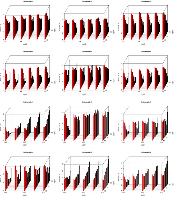
A

Backtesting results

Figure 5: E-mini SnP 500. Tweezer.

(21)

(22)

Figure 8: E-mini SnP 500. Support/Resistance.

(23)

Figure 10: OMXS30 Futures. Tweezer.

(24)

(25)

Figure 13: OMXS30 Futures. Support/Resistance.

(26)

Figure 15: RTS Futures. Tweezer.

(27)

(28)

Figure 18: RTS Futures. Support/Resistance.

(29)

B

Weights calculation

Table 11: E-mini S&P 500. The Highest Return optimization

φ Subsample 2 3 4 5 6 7 R∗_i−1,φ Tweezer −8.25% −2.77% −11.71% −5.51% −13.06% −4.02% MA 7.87% 8.51% 11.56% 37.88% 9.5% 6.2% Rsi 6.62% 0.9% 0.16% 2.88% 15.15% 5.3% Channels −2.09% −1.76% −12.63% −21.58% −9.75% −7.35% Momentum 0.02% −1.38% 1.12% 1.58% 2.01% 0.31% ω_i,φ Tweezer 0% 0% 0% 0% 0% 0% MA 54.22% 90.45% 90.02% 89.47% 35.63% 52.54% Rsi 45.64% 9.55% 1.28% 6.8% 56.82% 44.86% Channels 0% 0% 0% 0% 0% 0% Momentum 0.15% 0% 8.69% 3.73% 7.55% 2.61%

Table 12: E-mini S&P 500. The Highest Reward to Risk Ratio optimization

φ Subsample 2 3 4 5 6 7 RRR∗_i−1,φ Tweezer −0.95 −0.66 −0.87 −0.36 −0.93 −0.57 MA 4.98 4.09 4.42 7.24 3.22 1.15 Rsi 3.52 0.69 0.05 15.27 12.28 22.23 Channels 0 0 0 −0.01 0 0 Momentum 0.02 0 0.69 0.59 2.65 0.12 ωi,φ Tweezer 0% 0% 0% 0% 0% 0% MA 58.59% 100% 100% 32.16% 17.76% 4.92% Rsi 41.41% 0% 0% 67.84% 67.67% 95.08% Channels 0% 0% 0% 0% 0% 0% Momentum 0% 0% 0% 0% 14.58% 0%

(30)

Table 13: OMXS30 Futures. The Highest Return optimization φ Subsample 2 3 4 5 6 R∗_i−1,φ Tweezer 11.96% 12.74% 31.47% 10.51% 11.95% MA 32.09% 14.3% 38.77% 17.86% 16.52% Rsi 7.46% 19.74% 35.99% 18.94% 9.87% Channels 26.42% 18.82% 36.22% 12.91% 6.69% Momentum 1.29% 6.28% 7.7% 2.9% 2.78% ωi,φ Tweezer 15.1% 17.72% 20.96% 16.65% 25% MA 40.51% 19.9% 25.82% 28.3% 34.55% Rsi 9.41% 27.46% 23.97% 30% 20.65% Channels 33.35% 26.18% 24.12% 20.45% 13.99% Momentum 1.63% 8.74% 5.13% 4.6% 5.81%

Table 14: OMXS30 Futures. The Highest Reward to Risk Ratio optimization

φ Subsample 2 3 4 5 6 RRR∗_i−1,φ Tweezer 7.65 4.69 6.68 4.56 5.47 MA 14.51 3.25 7.11 4.76 5.52 Rsi 6.78 14.34 11.21 18.08 7.63 Channels 16.7 7.01 8.89 6.11 1.63 Momentum 3.03 5.5 3.9 1.59 1.95 ωi,φ Tweezer 15.72% 13.48% 17.68% 12.99% 24.64% MA 29.81% 9.33% 18.81% 13.57% 24.85% Rsi 13.94% 41.23% 29.66% 51.52% 34.37% Channels 34.31% 20.15% 23.52% 17.4% 7.36% Momentum 6.23% 15.81% 10.33% 4.53% 8.78%

(31)

Table 15: RTS Futures. The Highest Return optimization φ Subsample 2 3 4 5 6 7 8 R∗_i−1,φ Tweezer 14.75% 2.03% 33.43% 23.18% 1.7% 3.49% 9.59% MA 28.27% 13.57% 145.97% 52.58% 17.77% 10.69% 17.31% Rsi 32.45% 23.56% 83.33% 44.69% 18.39% 8.81% 13.3% Channels 1.22% 5.42% 16.23% 16.3% 12.38% 9.77% 9.39% Momentum 2.59% 11.74% 5.44% 9.66% −0.12% 5.24% 5.76% ω_i,φ Tweezer 18.61% 3.61% 11.75% 15.83% 3.37% 9.18% 17.32% MA 35.66% 24.09% 51.33% 35.92% 35.37% 28.12% 31.27% Rsi 40.93% 41.84% 29.3% 30.52% 36.6% 23.2% 24.03% Channels 1.54% 9.62% 5.71% 11.13% 24.65% 25.72% 16.97% Momentum 3.26% 20.85% 1.91% 6.6% 0% 13.78% 10.41%

Table 16: RTS Futures. The Highest Reward to Risk Ratio optimization

φ Subsample 2 3 4 5 6 7 8 RRR∗_i−1,φ Tweezer 13.63 0.34 6.84 7.88 0.53 2.89 5.32 MA 12.42 3.37 12.54 7.39 3.84 3.15 4.54 Rsi 44.38 18.6 19.38 22.26 13.17 4.46 8.75 Channels 0.52 1.34 2 9.57 11.95 14.5 17.91 Momentum 1.03 8.49 1.25 4.27 0 3.04 6.26 ωi,φ Tweezer 19.07% 0% 16.28% 15.34% 0% 10.32% 12.44% MA 17.37% 10.6% 29.86% 14.38% 13.25% 11.23% 10.61% Rsi 62.11% 58.5% 46.13% 43.33% 45.48% 15.91% 20.45% Channels 0% 4.2% 4.76% 18.62% 41.27% 51.71% 41.88% Momentum 1.44% 26.69% 2.97% 8.32% 0% 10.83% 14.63%