COMPARISON OF THE GRAPH-OPTIMIZATION FRAMEWORKS G2O AND SBA

V¨

aster˚

as, Sweden

Thesis for the Degree of Master of Science in Engineering - Robotics

30.0 credits

COMPARISON OF THE

GRAPH-OPTIMIZATION

FRAMEWORKS G2O AND SBA

Henning Victorin

hvn10001@student.mdh.se

Examiner: Mikael Ekstr¨

om

M¨

alardalen University, V¨

aster˚

as, Sweden

Supervisors: Giacomo Spampinato, Carl Ahlberg

M¨

alardalen University, V¨

aster˚

as, Sweden

Company supervisor: Bj¨

orn Holmberg

Unibap AB, Uppsala, Sweden

Abstract

This thesis starts with an introduction to Simulataneous Localization and Mapping (SLAM) and more background on Visual SLAM (VSLAM). The goal of VSLAM is to map the world with a camera, and at the same time localize the camera in that world. One important step is to optimize the acquired map, which can be done in several different ways. In this thesis, two state-of-the-art optimization algorithms are identified and compared, namely the g2o package and the SBA package. The results show that SBA is better on smaller datasets, and g2o on larger. It is also discovered that there is an error in the implementation of the pinhole camera model in the SBA package.

Table of Contents

2.2 Sensor selection . . . 7

2.3 Mono, stereo or RGB-D . . . 7

2.4 Feature based or direct . . . 8

2.5 SLAM or PTAM . . . 8 3 Related Work 9 4 Method 11 4.1 Research Question . . . 11 4.2 Research Method . . . 11 4.3 The Equations . . . 11 4.3.1 The Error . . . 11

4.3.2 The Error Function . . . 12

4.3.3 The Levenberg-Marquardt Algorithm . . . 12

4.3.4 Differences . . . 13

4.4 Comparison . . . 14

4.5 Platform . . . 14

5 Results 16 5.1 Previous Results . . . 16

5.1.1 The SBA Experiment . . . 16

5.1.2 The sSBA Experiment . . . 16

5.1.3 The g2o Experiment . . . 16

5.1.4 Consistency Checks . . . 17 5.2 Expected Results . . . 17 5.3 Thesis Results . . . 19 6 Discussion 23 6.1 Computational Speed . . . 23 6.2 Convergence . . . 23 6.3 Average Error . . . 23 7 Conclusions 25 7.1 Research Answers . . . 25 7.2 Research Contributions . . . 25 7.3 Future work . . . 25 References 28

Appendix A Results from all runs 29

A.1 New College . . . 29

A.1.1 g2o . . . 29

A.1.2 SBA . . . 29

A.2 Venice . . . 29

A.2.1 g2o . . . 29

A.2.2 SBA . . . 30

Appendix B g2o Subset Creation Program 31

1

Introduction

Simultaneous Localization And Mapping (SLAM) aims to answer the questions ”What does the world around me look like, and where am I in it?”. SLAM is a mean of giving a robot a sense of direction. It is a very useful tool for numerous robotic applications. For example assistance in rescue missions[1], exploration of planetary bodies[2] and landmine detection[3]. SLAM has been around for a couple of decades now and the interest in it is growing quickly. It is one of the most important research fields of robotics today. This thesis aims to identify the best open source SLAM solutions available today, targeting the IVS-70 platform from Unibap AB. The IVS-70 is a safety critical stereo camera with computational power to do the image processing and analysis on board. SLAM is a big research field with several important sub-fields. To narrow the search down, this thesis is focusing on the final and perhaps most important step of SLAM called graph-optimization. To put this into context, an introduction to the different steps of SLAM follows.

1.1

Data Acquisition

To be able to map the surrounding, a robot with a SLAM system needs a way to observe the world. Therefore, SLAM systems are typically equipped with one or more sensors. The first step in any SLAM algorithm is to read the sensor values. This is referred to as data acquisition. Data acquisition can be simple and straight forward, depending on sensor type, but there is still important research beeing done in this field. Examples are improving the performance of Inertial Measurement Units (IMUs) or GPS, fusing data from an IMU and the optical flow in a camera or new calibration techniques. A SLAM system is no better than the quality of its aquired data.

1.2

Feature Detection

After acquiring the data, it is normally discretized in some way. To be able to associate the data acquired from different locations, a way to describe the data is needed. This step is called feature detection. How to do feature detection depends on what kind of sensor there is and what kind of environment the robot is supposed to operate in. A famous feature detectable by many kinds of sensors is the corner. It is a feature of high contrast and can be detected with, for example, sound, light or touch. Feature detection is also an important research field and it is very useful not only for SLAM but for many other applications aswell, especially within the field of computer vision. Two examples of early feature detectors are the Harris corner and edge detector and the Canny edge detector[4]. Detected features that qualify for usage in the SLAM algorithm are called landmarks.

1.3

Data Association

Data association is the phase when features from one pose is associated with features from an adjacent pose. This is the part where the robot realizes that two features detected in different poses actually represent the same landmark but from different views. The quality of the data association algorithm directly affects the performance of the SLAM algorithm. With robust data association, the features can be correctly associated despite beeing seen from quite different perspectives. This means that the robot can move further before data has to be acquired again, with the practical effect that the robot can move faster while performing SLAM. An important property of the robustness of the data association algorithm is the detection and removal of outliers. Outliers are feature pairs that are wrongly associated and, if included in the SLAM algorithms, worsens performance. A commonly used method for outlier removal is Random Sample Consensus (RANSAC)[5].

1.4

Loop Closure

While the data association solves the problem of relating data from one pose to the other, loop closure is used for the larger scale. The loop closure algorithm detects when the robot revisits a known location. If a robot is doing SLAM while moving around a building, loop closure would occur when the robot has completed one lap returning to its starting position. Loop closure is very useful, critical in some cases, for correcting different drift errors. Drift errors are errors that

accumulate over time and increasingly distorts the map. A well performing loop closure package is the FAB-MAP package[6].

1.5

Tracking

Having associated the newly acquired data with aldready known landmarks, an estimation of the robots position and orientation can be made. This step is called tracking. Tracking is most often formulated as a standard triangulation problem. Tracking is important for a successful SLAM algorithm, however it is not as complicated as the other parts and hence not commonly researched.

1.6

Mapping

While the tracking part tracks the movement of the robot, the mapping part tracks the landmarks and builds a map of the world. In many cases, tracking and mapping is done together, using the same algorithm. Mapping, however, extends to storing landmark positions in a map. These maps can take several forms such as state vectors, voxel grids or pose graphs. For details on which is

used for what, see section2. The mapping algorithm and the map structure affects how quick and

effective steps as data association, loop closure and tracking can be performed.

1.7

Graph Optimization

When using pose graphs, see section2.1, the final step of SLAM is graph optimization. Taking

the full history of measurements, landmarks and robot poses in consideration, the pose graph is optimized to produce the best fit. This is a very important step and around half of the algorithms on OpenSLAM [7] adress graph optimization only, instead of providing full SLAM solutions. Graph optimization produces much better accuracy of the map but it takes extra time. When used for SLAM, this step is often the most time consuming. Therefore, a big portion of the research beeing conducted on this is focusing on reducing the time to do graph optimization. The importance of graph-optimization for the accuracy and speed of the SLAM algorithm are the main reasons for focusing on graph optimization in this thesis.

2

Background

This section gives some background on SLAM and what choices that leads to the focus of this thesis.

2.1

Filter based or non-filter based SLAM

SLAM has been around for decades and during this time, a lot of different approaches have emerged. The perhaps most well known is the Kalman Filter (KF). The Kalman filter is based on two steps: prediction and update. Consider a system of a robot driving around a room, trying to localize itself and a set of landmarks. The prediciton would then be the expected position of the robot and the landmarks. For most cases, the prediction is based on the previous state of the system, a dynamic model of the robot and the control inputs. The predicted movement is then updated with actual measurements aquired with some sensor, in example a laser range finder. The laser measures the relative position of the landmarks, and this measurement is compared to the predicted position. Based on how consistent these values are, each landmark is assigned a covariance value. The covariance describes how good the landmark is as a landmark. If it is easy to detect and predict its position, the covariance will be low. If it is not detected in every timestep or if it seems like the position vary a bit, the covariance will be high. Based on the prediction, measurement and covariance, the state of the system is updated. The KF is optimal for solving linear filtering problems, however most systems are not linear. Because of this, several versions of the KF have evolved. There is the Extended Kalman Filter (EKF) which uses Taylor expansion to linearize the problem and then applies the KF. The Unscented Kalman Filter (UKF) is similar to the EKF but relies on the unscented transform instead of Taylor expansion. Then there are Particle Filters (PF) which sustain a population of several states, each associated with a probability of beeing correct. Each individual in this population could be an EKF on its own. This particular approach is known as FastSLAM and has gained a lot of attention. More detailed explanations of the different KF based solutions, and the required mathematics, can be found in [8]. There are many more variants of the KF algorithms and research is still beeing conducted[9][10][11][12]. All of EKF, UKF and PF are also currently used as SLAM solutions[13][14][15]. These solutions are called filter based solutions.

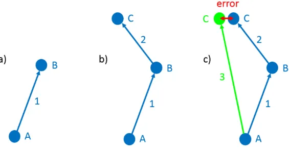
In contrast to filter based solutions, there are the non-filter based solutions, of which graph-based SLAM is most commonly used. The main idea here is to store poses (position and orientation)

as nodes connected by edges, referring to transformations derived from measurements, see fig. 1.

The graph is built by storing the initial pose A of the robot and a measurement, i.e. a laser scanning, of this pose. Then the robot is moved and a new measurement acquired at the new pose B. The measurements in A and B are used to calculate the transformation, edge 1. Then the transformation edge 1 is applied to pose A which results in pose data for pose B. Next time the robot moves it takes a new measurement from the new pose C. The same procedure is repeated and edge 2 and pose C is derived. If there is sufficient overlap between the measurements from pose A and C, a third edge can be added, edge 3, and a new estimation of pose C can be obtained. Due to noise and imperfection of the algorithms, the two estimations of pose C (green and blue in the figure) probably differs a bit. The difference is the error. The algorithm optimizes the graph by fine tuning all poses to minimize the error. Instead of just trying to get an as good last pose estimation as possible, as in filter based solutions, the whole pose history is optimized and updated every time step. A good tutorial on graph-based SLAM can be found in [16].

The filter based solutions are well known and widely used and therefore quite robust. Since they only need to consider the current state and the latest measurement, they are more memory efficient than non-filter based solutions. Non-filter based solutions have typically been used offline because of that. Offline means that first, all the data is collected. Then, the SLAM algorithm is applied. One example where this has been the preferred approach is within the field of photogrammetry. With computers ever increasing performance, non-filter based solutions have become a considerable alternative to, and have now been shown to outperform, the old filter based algorithms. Both in

terms of speed and accuracy[17][18]. Graph-based SLAM is the current state of the art and

Figure 1: Nodes and edges of a typical graph-based SLAM approach

2.2

Sensor selection

There are several ways to detect a change in pose, a movement. Typical for the KF solutions have been to use some dynamic model for prediction and some type of sensor for the update. The sensors could be accelerometers and gyros which measure acceleration and rotational velocity respectively. Wheel odometry is not uncommon, which is measuring how many turns the wheels have taken and derive translation and rotation from that. For this type of measurement different sensors are available, for example lasers (LIDAR), RADAR, ultrasonic sensors, cameras, GPS and compasses. The best result is often given by combining several methods, known as sensor fusion. Since the focus of this thesis is the underlying SLAM algorithm and not sensor selection, only one type of sensor is used. The sensor used in this case is the camera. Though LIDARs are traditionally the most precise, cameras have several advantages. First of all, they are cheap, for example there is a camera in almost every smartphone. Cameras are also smaller and less power consuming than lasers and they are more similar to the human eye, and hence camera data is more intuitive. Another good property is that, while beeing used for SLAM, they can still be used for many other things at the same time, such as face or text recognition. To use cameras for SLAM is also a very popular research field which is often called Visual SLAM, or VSLAM[19][20].

2.3

Mono, stereo or RGB-D

VSLAM can be divided in several categories. One important is how many, and what kind of, cameras are used. There are basically three options, mono, stereo and RGB-D SLAM. Mono SLAM means that only one camera is used. The procedure then is to take a picture, move a bit, take a new picture and derive the movement between them using some computer vision algorithm. A problem with mono is the absence of an absolute scale. Usually the first measurement is used as a reference but as the camera moves away from the initial pose, the scale begins to drift, which can result in different scales at different locations in the map. Pure mono slam algorithms are heavily dependent on good loop closures to adress this problem. Two examples of mono SLAM solutions are presented in [18] and [21].

In RGB-D SLAM, each pixel is extended with a depth value, typically from an infrared (IR) camera. The most famous example of a RGB-D camera might well be Microsofts Kinect. This type of SLAM generates a point cloud for each pose and the SLAM algorithm tries to match these point clouds together. A point cloud is a set of points with at least positional data, typically x, y and z. The Iterative Closest Point (ICP) algorithm is commonly used for this problem. The RGB-D approach eliminates the scale drift problem of the mono slam. Examples can be found in [22] and [23].

Stereo SLAM can be viewed either as mono or RGB-D SLAM. Depending on the stereo camera quality and setup, it can either generate point clouds or just one pair of mono images. The last case results in a mono slam algorithm but without the drifting scale. For every pose, there will always be a pair of images with a known absolute baseline. This thesis is targeting a such stereo vision system and that is why mono SLAM algorithms are beeing evaluated. The core of the SLAM algorithm is still the same, only the scale drift is missing. Examples of stereo SLAM are the work in [17] and [24].

2.4

Feature based or direct

After aquiring an image, the standard approach for VSLAM is to do feature detection. Features in this case are set of pixels that can be classified such as lines, corners, blobs or homogeneous patches. A good feature is recognizable despite different view points and scales. The algorithms rely on detecting the same features in two images. All features do not need to be present in both images, but there needs to be a sufficiently overlapping set of features. After detecting and associating these features, the pose change can be estimated. The most commonly used feature detectors are SIFT[25], SURF[26] and FAST[27][28]. This approach is called a feature based solution. Non-feature based or direct solutions do not rely on Non-features at all. They try to match the images pixel by pixel. One might argue that comparing every single pixel is more computationally heavy than just a set of features. On the other hand the whole process of feature detection can be skipped which in turn makes the algorithm faster. There are also arguments that information is lost when just comparing a few features instead of every pixel, which would give a less accurate estimate. But, again, one could consider feature extraction as extracting even more information from the image instead of just looking at pixels. For more details on direct SLAM, see the work in [29] and [30]. This thesis is comparing feature based approaches because they are well known and more research has been conducted on the subject.

2.5

SLAM or PTAM

In the traditional SLAM approach, localization and mapping are tightly coupled and depend

on each other. When a new landmark is detected, the landmarks position can be estimated

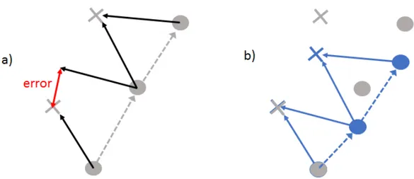
since the robots pose is known and since there is a measurement from the robots pose to the landmark. In the next step, when the robot has moved, the new pose can be estimated from already known landmarks and the relative measurement. The Parallell Tracking And Mapping (PTAM) approach, introduced in [31], is to have two separate threads, one managing mapping and the other managing tracking of the robot. The advantage of separating the two is that minor errors in pose estimation will not add up and contaminate the whole map and all following pose

and landmark estimations, as is the case for traditional SLAM, see fig. 2. Another benefit is

that the tracking (pose estimation) can be run at a much faster rate as the whole map does not need to be updated every time step. The map is then updated in the second thread when there is time for it. When using PTAM for VSLAM the mapping is done with image alignment tools. This is computationally heavy and the major drawback of PTAM. In [8] it is argued that an approach that separates tracking an mapping will never be successful since they are so tightly coupled. However, recent studies show that some the best localization and mapping algorithms are PTAM algorithms[18][32]. This is much thanks to the increasing computational power available, and thanks to significant progress made in the field of linear algebra, for more details see section 4. Because of these reasons, this thesis considers algorithms suitable for PTAM.

Figure 2: Figure a) shows the ground truth for the robot poses (circles) and landmark positions (crosses). Measurements taken by the robot are shown with black arrows. There is an error in the second measurement shown in red. Figure b) shows the true poses and landmarks in grey, overlayed by the estimated poses and landmarks in blue. Note how the whole map after the second measurement is distorted. This is because of the error in the second measurement.

3

Related Work

The focus of this thesis lies in the graph optimization of PTAM based VSLAM solutions. Nearly all of these solutions rely on bundle adjustment (BA). The BA problem is to optimize a set of camera poses and corresponding pictures. The name refers to bundles of light rays travelling from the features to the camera poses. The camera poses are then adjusted to find the best fit. BA has been around for decades and in 2000, [33] was published. The intention was to pass on the knowledge from the photogrammetry society to the computer vision and robotics societies. The work describes BA in detail, but these are the basics: Given an estimated camera pose and an estimated landmark position, the expected position of the landmark in the picture is calculated, typically using the pinhole camera model[34]. The expected position is given in pixels and the result is compared with the actual measured pixel coordinates of that landmark in the picture. The difference is an error. All the errors, taking every camera pose and every landmark in account, are gathered in an error function. Then the camera poses are adjusted to minimize the error function. This is done iteratively, typically using the Levenberg-Marquardt algorithm[35], a more detailed

description is given in section4.3.3.

BA is computationally very heavy which has been the greatest problem for using it for online SLAM. The reason is that the computations needed involve operations with huge matrices. To remedy this, a sofware package for Sparse Bundle Adjustment (SBA) was presented 2009[36]. SBA utilizes the sparsity of the huge matrices to increase the computational speed. Sparse means that, thanks to the way the matrices are constructed, most of the elements are actually zero. Only a few elements along the diagonal and the edges are non-zero. In the same work[36], SBA was also compared to BA on two datasets and SBA was 1660 respectively 5447 times faster than standard BA.

PTAM was invented 2007 and was presented in [31]. That means that it was invented before SBA and used normal dense BA and was nevertheless running at videorate, though only in small workspaces. In [37] they even managed to get PTAM running on an iPhone. This was 2009 and they managed to do it by reducing the computational load by other means, in example to not run BA on the full dataset every time, but on the last few frames instead. They also reduced the number of features by beeing more concerned about getting robust features instead. PTAM has also been used for various research projects ever since. In [32], a SLAM solution based on PTAM for larger scales is presented. Another research group adjusted PTAM and used it to map Hofburg Festsaal in Vienna[38]. In [39] it was used to control a 3 degrees of freedom helicopter and in [21] PTAM is extended with superpixels. Superpixels are here big homogenous surfaces. The result was much better looking 3D-reconstruction of the scene than with the original PTAM.

In 2010 Sparse Sparse Bundle Adjustment (sSBA) was published[40]. sSBA is even more sparse than SBA and also uses different software packages for the Levenberg-Marquardt algorithm. It proved to be more than 100 times faster than SBA on large datasets. The largest dataset used in that comparison was around 3000 camera poses. In the sSBA paper[40] it is also pointed out that the dataset itself affects the performance very much. If it is a very dense dataset, with a lot of camera poses and a high degree of overlapping poses, the matrices will be denser and hence the computational effort will grow quickly with the number of poses. In a sparse dataset, where each camera pose only overlaps with a few other, the problem will grow almost linearly with the number of poses. Overlap here means that the same features are detected in two camera poses. A full VSLAM solution using sSBA for graph optimization can be found in [41].

g2o[42] was released 2011. It is a general graph optimization framework and can do all sorts of graph optimization, including BA. It is similar to the sSBA package but can also solve other problems than just BA. In [42] g2o was also compared to sSBA and proved to be a little bit more efficient on small datasets and a little bit less efficient on large datasets. g2o is considered state of the art and has been used in several SLAM solutions[30][19][43].

sSBA and g2o are both released by Willow Garage and the author of sSBA is also a co-author of g2o. The general approach of both solutions is the same, namely the SBA approach. sSBA is an extension of SBA and g2o refers to SBA for details. However, there is a difference in the error function. SBA defines the error function as the squared sum of all errors, whereas sSBA and

g2o both uses a weighted squared sum. For more details on this, see section4.3.4. There is also

one major difference in the BA, SBA and sSBA papers: SBA and sSBA follows the standard BA procedure. The error is defined as the difference between the expected projection of a landmark in the picture, and the measured projection of the landmark. g2o defines the error as the difference between the expected and the measured pose change, the translation and rotation between two poses. The source code of g2o is somewhat hard to follow. The notation differs between the paper and the code and the actual equations described in the paper are deeply hidden in different packages. However, after thoroughly analyzing the code, it can be concluded that g2o actually also follows the standard BA approach. This conclusion highlights an important matter when comparing different approaches. sSBA and g2o seemingly follow the exact same procedure for BA, they use the same mathematical packages and they still differ in performance. This means that the actual implementation of the code is very important and something that needs not to be forgotten. This thesis will compare the SBA package and the g2o package on BA problems. The com-parison will cover computational speed, solid state error and convergence. Speed for confirmation with earlier results. Solid state error to see if a secondary sparse structure affects not only the computational speed but also the accuracy. Convergence describes how fast an algorithm reaches solid state. Convergence is interesting to compare since a computanionally slow algorithm with fast convergence might reach solid state earlier than a fast algorithm with slow convergence.. There are mainly two reasons that sSBA is not included. First, it is very similar to g2o and even written by the same authors. Second, sSBA depends on ROS[44], which is not compatible with lUbuntu 15.10, which is the operative system used in this experiment. The datasets used for the comparison, New

(a) New College as shown in [47]. (b) Venice as shown in [42].

Figure 3: Pictures of the datasets

4

Method

This section states the research problem and method. Then follows a detailed explanation of the method used to solve the BA problem. After that, a comparison of the chosen algorithms is made and the final subsection contains information about the physical platforms used.

4.1

Research Question

The research question of this thesis is: Which of the graph-optimization packages SBA and g2o is the best?

4.2

Research Method

To find out which is the best of SBA (sba-1.6) and g2o, the two algorithms are evaluated on the same datasets. SBA was downloaded from [48] and g2o from [49]. After that, the results are compared, both with each other and with previous results from earlier studies. Special attention is paid to speed, accuracy and convergence.

4.3

The Equations

Both g2o and SBA use almost exactly the same equations. This section will first go through all steps involved and then point out the differences.

4.3.1 The Error

The core in the graph optimization is to minimize the error function. To be able to do that, the error needs to be defined. The error in BA is measured in pixels. It is defined as the difference between the expected measurement of a landmark and the actual measurement of a landmark. The expected measurement can be calculated given the estimated camera pose and landmark position. Then the pinhole camera model is used to convert the 3D position of the landmark to a

2D projection in the camera image plane, see fig. 4. Let the ith camera be ci and the jth point

pj. Let the pinhole camera function be f (ci, pj), the measured projection of a point in a camera

frame be z and the estimated projection ˆz. The estimated projection is then ˆz = f (ci, pj) and the

error eij is

Figure 4: ci is a camera and pj the estimated position of a point. The true position of that point

is the gray cross. ˆz is the pixel position where pj is expected to be detected and z is the pixel

position where it actually was detected. eij is the error

4.3.2 The Error Function

Once the error is defined, the error function needs to be defined. The error function evaluates how good the current state is. The course of action is to minimize the error function since if the error function returns a high value, the solution is bad. If it instead returns a low value, the solution is good. The error function is defined as the total sum of the squared errors. The vector with all the camera poses is called c and the vector with all the points p. Let the total error be E(c, p) and the error function is then

E(c, p) =X

ij

eTijeij (2)

There are two benefits with choosing this particular error function. One is that the square function makes positive and negative errors equivalent. Otherwise a negative and a positive error of the same size would negate each other and appear as zero error in total. The other benefit with the square function is that its minimum occurs not only when the errors are as small as possible, but also as equally distributed as possible. Consider a case where there are two measurements of a

point. The very simple error function E =P |e| has its minimum at all the points anywhere along

the straight line between the two measurements. The squared error function in equation (2) has

its minimum at the single point exactly halfway between the two measurements, see fig. 5.

4.3.3 The Levenberg-Marquardt Algorithm

The next step is to find the inputs c and p that minimizes the error function E. To find the minimum, the Levenberg-Marquardt algorithm is used. To ease notation, the considered camera pose c and point p are stacked in a parameter vector x. Then the error can be written e(x). What is sought now is an adjusted parameter vector, in the neighbourhood of x, that minimizes the error. The error for the adjusted parameter vector is

0 20 40 60 80 100 0 10 20 30 40 50 60 70 80 90 100

(a) Total asbolute error

0 20 40 60 80 100 0 10 20 30 40 50 60 70 80 90 100

(b) Total squared error

Figure 5: The value of the error functions. The red crosses represents the two measurement taken. The colormap describes the magnitude of the error function where red is high and blue is low. Figure (a) describes the total absolute error and figure (b) the total squared error.

and it is ∆x that is this adjustment that is sought. This error is approximated with Taylor

expansion yielding

e(x + ∆x) ' e(x) + J∆x (3)

where J is the Jacobian of e with respect to x. A Jacobian is the matrix form of derivative. In equation (3), J is the direction and ∆x is the step size of the update. In this case, J is defined as

J = δe

δx

Since both e and x are known, J can be derived analytically from equation (1). Next the second order derivative matrix, the Hessian, is approximated as

H ' JTJ

By left multiplicating equation (3) with JT and setting e(x + ∆x) = 0 (meaning the sought error

is 0) the equation system

H∆x = −JTe (4)

is obtained. To get better control over the step size ∆x the Levenberg-Marquardt algorithm

introduces a damping factor, λ. The resulting equation system is

(H + λI)∆x = −JTe (5)

Now it is just to solve for ∆x. The sSBA and g2o packages use a Cholesky solver from the CHOLMOD package[50][51] while SBA uses the Cholesky solver from the LAPACK package[52]. The new parameter vector x is evaluated and if the result is a decrease of the total error, the update is accepted, the damping factor λ is decreased and the algorithm is run for another iteration. If the result is an increase of the total error, then the update is rejected and λ is increased. The algorithm is iterated until the error is sufficiently small, for a certain amount of iterations, or until some other end conditions are met. For more details on the Levenberg-Marquardt algorithm see [53][54][55].

4.3.4 Differences

First of all there is a slight difference in the error function. In SBA the error function is defined as in equation (2), but in sSBA and g2o it is defined as

E(c, p) =X

ij

where Ωij is the information matrix. It contains values that describe how good the current

mea-surement is. The information matrix is the inverted covariance matrix which is described in section 2.1. However, in the sSBA paper[40], it is mentioned that this matrix is often the identity matrix

and can therefore be ignored. The appearance of Ωij in the error function causes it to appear in

the definition of the Hessian too. Hence in g2o only, the Hessian is defined as

H = JTΩJ

Another difference is in equation (4). In sSBA it is written just as that, which is also what is obtained by doing the operations explained above. However, in the SBA paper, the sign is altered

and the system is H∆x = JTe. In g2o the structure is a bit different and the resulting system is

the transpose of equation (4) defined as H∆x = −eT_{J. The different variants should not matter}

that much but are worth mentioning for the interested reader.

Apart from that there is yet another difference in the Levenberg-Marquardt equation system, equation (5). SBA and g2o follows the definition above but sSBA differs by using the diagonal of H instead of I. This is actually what is proposed by Levenberg and the method implemented by g2o and SBA is a simplification. The resulting equation is

(H + λdiag(H))∆x = −JTe

Finally, the most important difference is the difference in solvers used. The LAPACK solver is sparse but the CHOLMOD solver is even more sparse. In short, SBA uses a sparse approach for J while sSBA and g2o use a sparse approach for both J and H. For details see [40]. This is what makes sSBA and g2o supposedly superior to SBA. The use of secondary sparse structures and the CHOLMOD package was proposed as a future enhancement in the SBA paper[36].

4.4

Comparison

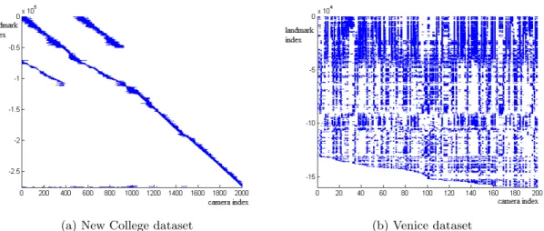
Two graph optimization alorithms, g2o and SBA, are compared, both performing BA. The datasets used are the New College dataset and the Venice dataset. It is the same datasets that were used as examples with g2o and the Venice dataset was also used by sSBA. The other datasets from the SBA, sSBA and g2o papers were either unavailable or an a format difficult to convert. Both the New College and the Venice datasets are large datasets and it is easier to scale down large datasets than to scale up small. New College has 3500 camera poses and Venice has 871. They are both also real world datasets. New College is a quite sparse dataset while Venice is quite dense. It means that in the New College dataset, a landmark is typically seen from a few adjacent camera poses. This structure generates sparser matrices which are mainly populated close to the diagonal and along the edges. The Venice dataset beeing dense means that a landmark is typically seen from several arbitrarily distributed camera poses. This property generates more dense matrices.

The density of the datasets is visualized in figure6.

To be able to compare on different sizes of datasets, both datasets were scaled down. The downscaling was made so that first n camera poses was chosen. Then a subset was created con-taining the first n camera poses of the complete dataset, and all points seen from at least two different poses. Subsets of the New College dataset was created containing 5, 10, 50, 100, 200, 500, 1000, 2000 and 3500 camera poses. From the Venice dataset, subsets with 5, 10, 20, 50, 100, 200, 500 and 871 camera poses was created. The datasets were available in the g2o format and thus needed conversion to the SBA format. The source code for the program used to scale down

the g2o datasets can be found in appendixB. The source code for the program used to convert

datasets from the g2o format to the SBA format can be found in appendixC.

4.5

Platform

This thesis is targeting the stereo camera IVS-70 from Unibap AB. It currently feaures an AMD G-series GX-415, Quad-core 1.5 GHz system on chip (SoC) computing module and a SmartFusion2

FPGA by Microsemi. Since the system was not available at the time, the experiments were

conducted on a laptop on one core of an AMD A10-5745M processor at 2.10 GHz running Ubuntu 15.10. 320 kB L1 cache, 8 MB L2 cache and 11.2 GB RAM. For reference, the g2o experiments

(a) New College dataset (b) Venice dataset

Figure 6: Graphs showing the density of the datasets. On the x-axis is the index i of the camera

ci in the camera vector. On the y-axis is the index j of the landmark pj in the landmark vector. j

is negated to retrieve visual properties similar to the sparse matrix as shown in [40]. If a landmark is seen from a camera pose, there is a blue mark on position (i, j).

were conducted on one core of an Intel Core i7-930 at 2.8 GHz, the SBA on a 1.8GHz Intel P4, 8 kB L1 cache, 256 kB L2 cache, 512 MB RAM, and the sSBA experiments on one core of an Intel i7 at 3.0 GHz, 49GB RAM. The sSBA paper claims that the platform they use features 8 MB of primary cache, which would be L1. It is more likely that it is L2 or L3 (or a combination) though.

5

Results

The first part of this section presents the results from the SBA, sSBA and g2o experiments. Given this information, the expected results of the experiment of this thesis are derived and in the final part, the produced results of this thesis experiment are presented.

5.1

Previous Results

This subsection presents results shown in the literature. Three experiments are presented here. The SBA experiment refers to the SBA algorithm beeing evaluated on eight datasets, namely the movi, sagalassos, arenberg, basement, house, maquette, desk and calgrid datasets[36]. The sSBA experiment refers to the sSBA and SBA algorithms beeing evaluated on four datasets, namely the Venice, Samantha Erber, Samantha Bra and Intel datasets[40]. The g2o experiment refers to the g2o and sSBA algortihms beeing evaluated on two datasets, namely New College and Venice[42].

5.1.1 The SBA Experiment

The SBA algorithm was initially evaluated on eight different datasets varying between 10 and 59 camera poses. None of these datasets could be used for the experiment of this thesis, but comparable sized datasets have been generated from the New College and Venice datasets. The

results of the SBA experiment are shown in table1.

Table 1: The results of the SBA experiment

Sequence Camera Poses Landmarks Average Errorˆ2 Iterations Time/Iteration (s)

”movi” 59 1778 0.3159 20 0.16 ”sagalassos” 29 1709 1.2703 30 0.11 ”arenberg” 22 1335 0.5399 18 0.14 ”basement” 11 305 0.2447 23 0.013 ”house” 10 515 0.2142 19 0.019 ”maquette” 54 5207 0.1765 22 0.33 ”desk” 46 3422 1.5760 22 0.25 ”calgrid” 27 722 0.2297 20 0.36

5.1.2 The sSBA Experiment

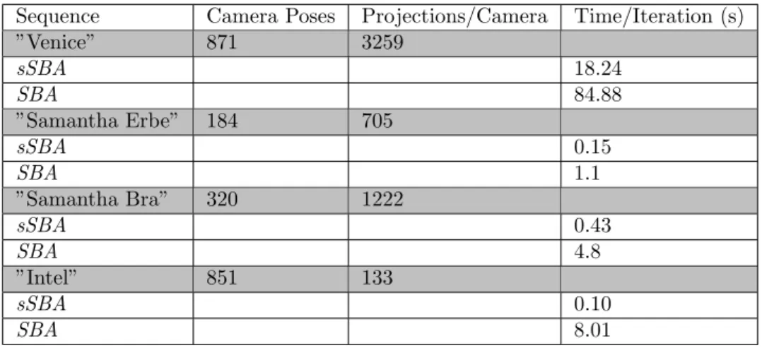
In the sSBA experiment, the SBA and the sSBA algorithms were evaluated on four different datasets, ranging from 184 to 871 camera poses. There is less result data available and neither total time, number of iterations nor average error are provided. The time is available as the average time per iteration. The missing error information might be the biggest problem. Without knowing the resulting average error it is hard to evaluate the algorithm. There is not much point in having a very fast algorithm if the result is of terrible quality. To be able to compare with the sSBA results, it is assumed that the average error in the sSBA experiments is similar to the results from the other experiments. A notable difference is also that not the number of landmarks but the average number of projections per camera is included in the results. The results of the sSBA experiment

are shown in table2.

5.1.3 The g2o Experiment

The results from the g2o experiment are somewhat scattered throughout the paper. However, there is in total quite much data presented on the Venice and New College datasets, compared

to the other datasets used in the experiment. Combining different graphs and tables, table3 can

be extracted for those two datasets. The average squared error in table3is computed by looking

closely at the total squared error shown in fig. 9 in the g2o paper, and dividing that total error with the number of constraints for each dataset. A constraint here is the same as a projection of a landmark on an image taken at a certain camera pose. All these numbers are for the g2o algorithm,

Table 2: The results of the sSBA experiment

Sequence Camera Poses Projections/Camera Time/Iteration (s)

”Venice” 871 3259 sSBA 18.24 SBA 84.88 ”Samantha Erbe” 184 705 sSBA 0.15 SBA 1.1 ”Samantha Bra” 320 1222 sSBA 0.43 SBA 4.8 ”Intel” 851 133 sSBA 0.10 SBA 8.01

however, it is shown in the g2o paper that sSBA and g2o have very similar performance, at least when it comes to time per iteration. For further comparisions, it is assumed that the sSBA times per iteration on the different datasets are the same as for g2o.

Table 3: The results from the g2o experiment

Sequence Camera Poses Landmarks Average Errorˆ2 Iterations Time/Iteration (s)

”Venice” 871 530304 7.2 100 13.03

”New College” 3500 488141 0.94 20 10.44

5.1.4 Consistency Checks

There are a few things that can be checked to investigate the consistency between the papers and

the presented results. Looking at table1it is clear that the SBA time per iteration increases quite

rapidly with the size of the dataset. The datasets SBA is evaluated on in the sSBA experiment are all larger than those in the SBA experiment. Given that, it is highly probable that the SBA

time per iteration should be higher in the sSBA experiments. This is confirmed in table2.

In the g2o paper, the Venice dataset is claimed to contain 871 camera poses and 2838740 constrains or projections. That would give 2838740/571 ≈ 3259.17 projections per camera, which

is also confirmed in table2.

In the sSBA experiment, the time per iteration is 18.24 seconds for the Venice dataset, running at 3.0 GHz. The g2o experiment run at 2.8 GHz. This means that the average time per iteration for the sSBA algorithm in the g2o experiment would be 18.24 ∗ 3.0/2.8 = 19.54 seconds. This is not the case. In the g2o experiment, the sSBA algorithm takes a little less than 13.03 seconds per iteration. This could be because the average might be taken on different sets of iterations. In the g2o experiment, the average is taken on the first 10 iterations. In the sSBA experiment this is unspecified. It is also likely that it is because of the computers used to run the experiments. In the sSBA experiment, the platform features 8 MB of L2 cache memory and 49 GB of RAM. In the g2o experiment, these numbers are unspecified.

5.2

Expected Results

Among the subsets created from the New College and Venice datasets, there are some that match quite well with datasets from the SBA experiment. In example the ”Venice 10” dataset features 10 camera poses and 493 landmarks compared to the ”house” dataset which has 10 camera poses and

515 landmarks. Looking at table1 it seems like the number of landmarks has a bigger influence

on the execution time than the number of camera poses. The BA procedure clearly depends most

of all on the number of projections (see section4.3) which is consistent with the SBA experiment.

is not given, nor is any information on sparseness or denseness of structures, so the predictions are expected to be correct more on the order of magnitudes than on the decimals. Taking all this into account, it can be expected that the sequences ”movi”, ”sagalassos”, ”arenberg” and ”New College 10” should give somewhat similar results. So should dataset ”New College 50”, ”Venice 20” and ”maquette”. ”New College 20” should be in between, maybe closer to ”desk” and ”Venice 50” should take much longer time per iteration. Considering that this thesis experiment runs on 2.1 GHz and the SBA experiment ran on 1.8 GHz there should be a slight improvement in performance. Using the above mentioned sequences from the SBA experiments total times and the relation between the processor frequencies, the SBA results on the subsets can be estimated,

see table4. The average squared error is hard to predict since it varies between sequences and the

subsets of Venice and New College datasets have not been used before.

In the sSBA experiment, both the SBA and the sSBA algorithm are evaluted on the Venice

dataset, see table2. There is some information on sparsity available in the projections per camera

column, though this value gives no information about which landmarks that are seen from which camera poses. There are 2124449 projections in the New College dataset, spread on 3500 camera poses, the projections per camera property on the New College dataset is 2124449/3500 ≈ 607. The Samatha Erbe sequence of the sSBA experiment is the dataset most similar to the New College with 705 projections per camera. Given all this, expected results on the full Venice and New College

datasets for both SBA and g2o can be estimated, see table4. The estimation on the New College

dataset needs some explanation. If the Samatha Erbe sequence and the New College dataset are assumed to be of the same sparsity, an expected estimation on the New College dataset time per iteration in the g2o experiment can be calculated by taking several parameters in account. The

ratio of camera poses(3500₁₈₄), the ratio in processor speed(3.0_2.8) and the unexpected high performance

of the g2o experiment (13.03_19.54, explained in the previous subsection). The expression obtained is

3.0 2.8∗ 3500 184 ∗ 13.03 19.54∗ 0.15 = 2.04

This is quite different from 10.44 seconds per iteration as is reported in the g2o paper. Assuming that this is due to different sparsity patterns, it can be compensated for in this thesis experiment

by replacing the unexpectedly good perfomance(13.03_19.54) with the unexpectedly bad performance

shown above(10.44_2.04). The estimation of the expected time per iteration is then

3.0 2.1∗ 3500 184 ∗ 10.44 2.04 ∗ 0.15 = 20.86

The calculation looks similar for the SBA case. These estimations should be quite accurate since a lot of information is given, especially for the estimation on the full Venice dataset. Considering the unexpected performance of the g2o algorithm the real numbers might differ anyway. The g2o experiment suggest other estimations of the g2o algorithm performance on the full Venice

and New College datasets. To illustrate this, the or-operator || is used in table 4 to represent

sSBA − based − estimation||g2o − based − estimation. If the difference lies in the implementation, then the g2o time per iteration should be the right value and SBA the left. If it is due to the computer, g2o and SBA should both be closer to the left or both to the right values.

Left is to estimate time per iteration for the g2o algorithm on the subsets. There is not much information, so based on the g2o and sSBA papers, the estimations are set to roughly 10 times faster than SBA.

Table 4: Expected results

Sequence Camera Poses Landmarks Average Errorˆ2 Iterations Time/Iteration (s)

”Venice 10” 10 493 SBA 19 0.016 g2o 19 0.0016 ”New College 10” 10 1600 SBA 20 0.12 g2o 20 0.012 ”Venice 20” 20 5204 SBA 22 0.28 g2o 22 0.028 ”New College 20” 20 2892 SBA 22 0.21 g2o 22 0.021 ”Venice 50” 50 34810 SBA 20 3.92 g2o 20 0.39 ”New College 50” 50 6907 SBA 22 0.28 g2o 22 0.028 ”Venice 871” 871 530304 SBA 7.2 100 121.26 || 80.82 g2o 7.2 100 26.06 || 17.37 ”New College 3500” 3500 488141 SBA 0.94 20 151.36 || 102.08 g2o 0.94 20 20.86 || 13.92

5.3

Thesis Results

The results from running SBA and g2o on the datasets are shown in table5. The g2o algorithm

behaved like expected, 3-4 times slower than estimated but still within the expected range. Con-sidering the New College datasets, the SBA algorithm also performed more or less as expected, but was 2-4 times faster than estimated on the smaller sequences. The result of SBA beeing faster and g2o beeing slower is that they perform equally well, interestingly, SBA is even a little bit faster on the smaller sequences. The same goes for the average squared error. As the datasets grow, the difference grows and on the larger datasets, g2o clearly outperforms SBA, both in terms of speed

and accuracy. See fig7for diagrams on how the performance changes with the size of the dataset.

As the initial total error grows, the worse the SBA algorithm performs. It returns ridiculously

high errors and crashes for several large, dense datasets. The cells marked with ∗ in table5means

that the SBA algorithm crashed due to too big numbers. According to the papers, g2o and SBA uses exactly the same algorithm for deriving the projection error and updating the damping factor. Clearly, they do not. By looking at the source code, it turns out that they do actually use the same function for updating the λ, but the pinhole camera function differs, referred to earlier as

f (ci, pj), see section4.3.1. To be able to explain the difference, a short introduction to the pinhole

camera function is needed.

The camera pinhole function is explained in [36] and [34]. The following notation is not

con-sistent with the one used in section4. The pinhole function describes the 2D projection (u, v) on

the camera image plane of a 3D point (x, y, z) given in the world coordinate frame. The output

pixel coordinates are gathered in the vector x = λ ∗ [u v 1]T , where λ is a scale factor, and the

input point coordinates in the vector X = [x y z 1]T. To project the point in the plane, two

things are needed: Transformation of the point coordinates to the camera coordinate frame and projection of that point on the image plane. For the transform, a normal transformation matrix is used, composed of two parts, the rotational matrix R and a translational vector t. The rotational matrix is derived from the quaternion and the translational vector is the positional data of the camera pose. The resulting transformation matrix is [R|t]. Having transformed the point to the camera coordinates, the intrinsic matrix K is used to project it on the image plane. The final

0 500 1000 1500 2000 2500 3000 3500 0 10 20 30 40 50 60 70 80 Camera Poses Average Time/Iteration (s)

SBA on New College g2o on New College g2o on Venice (a) Speed 0 20 40 60 80 100 0 0.5 1 1.5 2 2.5 3 3.5 4 4.5 5 Camera Poses

Average error in pixels

SBA on New College g2o on New College g2o on Venice

(b) Accuracy

Figure 7: Graphs showing the performance of the different algorithms on the different datasets. SBA on Venice is not included since it crashed on most of the subsets.

equation is

λx = K[R|t]X

The SBA code did not use the exact same notation here and was hard to decipher. Consequently, a new implementation of the pinhole camera model was made from scratch, replacing the original in the SBA code. Both implementations produced the exact same results. g2o uses a slightly

different version, see equation6, and when this was used for SBA the errors where correct.

λx = K[RT| − RT_{t]X (6)}

The difference between the equations is the transformation from one coordinate system to an-other. The matrix R and vector t describe the camera orientation and position in the world coordinate frame. The transformation matrix [R|t] then describes the transformation from the camera coordinate system to world coordinates not from world coordinates to the camera coordi-nate frame. Hence, the SBA algorithm does exactly the opposite of what was intended, a fairly common mistake[56]. This can be confirmed by looking at the landmark positions and the camera

trajectory after optimization, figure8, where the red markers move away from the landmarks. The

transformation from world coordinates to camera coordinates is the world origin described in the

camera coordinate frame. That gives the transformation matrix [RT| − RTt] which is used in

equation (6). Since the Jacobian is derived from this pinhole function, it also needs to be replaced. Without replacing it, the SBA algorithm finishes very early since the updating of the step is wrong. Recalculating J would have been too time consuming and no more effort was made in correcting SBA.

The convergence of the error is also interesting to observe. If the error drops fast each iteration, it can be worth to spend more time on each iteration. The most important time is the total time to complete the optimization. For SBA and g2o, the convergence should be the same since both algorithms use Levenberger-Marquardt for minimizing the error. However, the false pinhole function affects this property too. g2o produces a much better initial estimate and therefore reaches

the solid state error faster. See figure11 for an example of the difference in convergence on the

”New College 10” subset.

To get a picture of how big impact the false pinhole camera model has, the initial error esti-mation, before any optimization, is considered. The initial average squared error on each subset is calculated for g2o, SBA and the corrected SBA algorithm, called SBAv2. On the Venice dataset,

g2o and SBAv2 generates exactly the same error, figure9a, while the original SBA algorithm

gen-erates errors tens of trillions times too big, figure9b. The comparison on the New College dataset

shows similar results. The difference is that g2o and SBAv2 does not give exactly the same error

estimations. In this case, SBAv2 gives a smaller error on each estimation, see figure10. There was

no difference in time per iteration between SBA and SBAv2.

Table 5: Thesis results

Sequence Camera Poses Landmarks Average Errorˆ2 Iterations Time/Iteration (s)

”Venice 10” 10 493 SBA 29994716.84 19 0.0079 g2o 0.23 19 0.0066 ”New College 10” 10 1600 SBA 0.70 20 0.038 g2o 1.19 20 0.04 ”Venice 20” 20 5204 SBA 1456860461.80 22 0.13 g2o 0.78 22 0.088 ”New College 20” 20 2892 SBA 0.84 22 0.088 g2o 1.35 22 0.095 ”Venice 50” 50 34810 SBA * * * g2o 4.28 20 0.9 ”New College 50” 50 6907 SBA 9.60 22 0.31 g2o 1.39 22 0.25 ”Venice 871” 871 530304 SBA * * * g2o 18.70 50 71.55 ”New College 3500” 3500 488141 SBA * * * g2o 1.59 20 39.70 −10 −5 0 5 10 15 20 −20 −15 −10 −5 0 5 raw

(a) Before optimization

−10 −5 0 5 10 15 20 −20 −15 −10 −5 0 5 afterSBA

(b) After SBA optimization

Figure 8: Top view of the ”New College 50” dataset. Red stars mark the camera poses and blue dots landmark positions. Note how the camera trajectory has changed completely after optimization and moves away from the landmarks.

0 100 200 300 400 500 600 700 800 900 −100 0 100 200 300 400 500 600 700 800 900 Camera Poses

Initial Average Error

2

g2o SBAv2

(a) g2o and SBAv2

0 100 200 300 400 500 600 700 800 900 −0.5 0 0.5 1 1.5 2 2.5 3 3.5 4x 10 14 SBA (b) SBA

Figure 9: The initial estimation on the average squared error on the Venice dataset. Note that this estimation is made before any optimization is done. Also note the scale difference on the y-axis.

0 500 1000 1500 2000 2500 3000 3500 0 5 10 15 20 25 30 Camera Poses

Initial Average Error

2

g2o SBAv2

(a) g2o and SBAv2

0 500 1000 1500 2000 2500 3000 3500 0 2 4 6 8 10 12x 10 10 SBA (b) SBA

Figure 10: The initial estimation on the average squared error on the New College dataset. Note that this estimation is made before any optimization is done. Also note the scale difference on the y-axis. 0 10 20 30 40 50 0 0.5 1 1.5 2 2.5 3 3.5 4 4.5 5 Convergence Iterations

Average Error (Pixels)

g2o SBA

Figure 11: The conver-gence, that is how fast the error is reduced, of the two algorithms on the New College 10 sub-set.

6

Discussion

This section discusses the thesis results to be able to answer the research questions. Since one algorithm can be more accurate but slower, the discussion is kept separate for the three properties computational speed, convergence and accuracy.

6.1

Computational Speed

Based on previous experiments, g2o was expected to be at least 10 times faster than SBA on any

dataset, see section5.2. This was not the case. Given a sparse dataset, such as New College, the

average time per iteration seems to grow linearly for the g2o algorithm, and exponentially for the

SBA algorithm, see figure7. This is consistent with SBA beeing sparse in the first order and g2o in

the second. It is also consistent with the sSBA paper, which states that the time per iteration for the sSBA (or g2o in this thesis) algorithm should grow linearly with respect to camera poses given a sparse dataset. It should grow more exponentially on a denser dataset, in this case the Venice dataset. This is validated by the fact that SBA on the New College and g2o on the Venice dataset almost follow the same curve. An effect of this is that the difference in speed is larger on larger datasets, but not that large on smaller datasets. For the smallest, SBA is actually faster. These are interesting results since it is neither mentioned in the sSBA paper nor the g2o paper, about the superior performance of SBA on smaller datasets. Small datasets are also quite common, for example when doing online SLAM where the BA algorithm often is run on only the latest few frames. Another example is applications for smaller workspaces. The SBA package is also smaller and easier to follow and adjust.

6.2

Convergence

Figure11 shows that the convergences are quite similar. The convergence of the SBA algorithm

starts with an offset, introduced by the false pinhole camera model, but the behaviour is similar to the g2o convergence. Since both algorithms claim to use the same functions, the convergence should be exactly the same. Both algorithms converges so fast that a minor difference would not have any significant effect on how fast a tolerated error is reached.

6.3

Average Error

Due to the false pinhole model, some errors from the SBA results are way too high. Though, on the smaller New College datasets, they are within an acceptable range. Since both papers aim to use the same BA procedure and mathematics, the error should be exactly the same, as is the case

shown in figure9a. The reason they are not the same in figure 10a is probably due to a slight

difference in the datasets. When the datasets were converted from the g2o to the SBA format, only landmarks seen by at least two cameras, and only cameras seeing at least one landmark seen by another camera, were included. The Venice dataset featured only cameras and points that fulfilled these criterias, but, the New College dataset included some points and cameras that did not. These were removed during conversion and it is probably these features that introduces this extra error.

The figures10b and9bshows that the problem with erroneous error estimations exists from the

start, hence it is not introduced by the first Levenberg-Marquardt iteration. Given all this, it can be concluded that no results on accuracy from the SBA algorithm can be trusted. f and J should be replaced with the correct ones.

f and J of the SBA package are actually considered user supplied functions. However, the functions used in this thesis experiments are the ones included in the demo program, that comes with the original SBA package. The SBA package was downloaded from the website suggested by the SBA paper. This makes the results of the SBA paper doubtable. Not when it comes to the computational gain but to the initial and final errors presented in the paper. Also, the standard non sparse BA algorithm is used to compare with, but only the execution times are presented, not the initial or final error. There is also an argument in that SBA uses the same update of the

state vector but with a positive Jacobian term, section 4.3.4. Why would everything be exactly

the same except the sign of that term? There is a possibility that it has something to do with the inverted projection function. The sSBA experiment does not present any results on accuracy

either. Since g2o includes the correct pinhole camera model, and since it is partly developed by the creator of sSBA, it is likely that the sSBA algorithm also used the correct model. However, since neither the SBA nor the sSBA paper presented any comparison on accuracy, it is likely that the SBA implementation used the false model in both cases.

7

Conclusions

This section presents the conclusions that can be drawn thanks to this thesis experiment.

7.1

Research Answers

The answer to the research question ”Which of the graph-optimization packages SBA and g2o is the best?” is:

• For small datasets and applications, use SBA. SBA performs comparable to g2o on smaller datasets, the code is consistent with the paper, and it is less code than g2o.

• For larger datasets or for a wider span of applications, use g2o. g2o is much faster on larger datasets, the code is very robust and it can be used for both small and big datasets.

7.2

Research Contributions

The contributions of this thesis are:

• Showing that SBA is faster than g2o on small datasets.

• Discovering that the pinhole camera model included in the SBA package is wrong.

7.3

Future work

For future work it would be interesting to correct the SBA package and run the experiments again. Due to the false pinhole camera model, SBA could not be evaluated thoroughly on the dense Venice dataset.

Since the number of projections has such an impact on the computational speed, it would also be interesting to compare the number of projections to the error. Could the same, or same enough, average squared error be reached with a reduced set of projections? If so, the computational speed could be improved only by considering fewer landmarks.

Since the target platform is the IVS-70 from Unibap AB, an implementation on that platform would give more insight in what performance could be achieved on an embedded system.

The algorithms for solving the optimization problem could also be reviewed. [42] does some experiments on different solvers where CHOLMOD is not always the best. It is also suggested by [36] to replace the Levenberg-Marquardt algorithm with something more efficient. These are experiments that would contribute further on the graph optimization problem.

References

[1] S. A. Berrabah, Y. Baudoin, and H. Sahli, “Slam for robotic assistance to fire-fighting ser-vices,” in Intelligent Control and Automation (WCICA), 2010 8th World Congress on, July 2010, pp. 362–367.

[2] C. H. Tong, T. D. Barfoot, and . Dupuis, “3d slam for planetary worksite mapping,” in Intelligent Robots and Systems (IROS), 2011 IEEE/RSJ International Conference on, Sept 2011, pp. 631–638.

[3] S. M. Abbas and A. Muhammad, “Outdoor rgb-d slam performance in slow mine detection,” in Robotics; Proceedings of ROBOTIK 2012; 7th German Conference on, May 2012, pp. 1–6. [4] C. Harris and M. Stephens, “A combined corner and edge detector,” in In Proc. of Fourth

Alvey Vision Conference, 1988, pp. 147–151.

[5] M. A. Fischler and R. C. Bolles, “Random sample consensus: A paradigm for model fitting with applications to image analysis and automated cartography,” Commun. ACM, vol. 24,

no. 6, pp. 381–395, Jun. 1981. [Online]. Available: http://doi.acm.org/10.1145/358669.358692

[6] M. Cummins and P. Newman, “FAB-MAP: Probabilistic Localization and Mapping in the Space of Appearance,” The International Journal of Robotics Research, vol. 27, no. 6, pp.

647–665. [Online]. Available: http://ijr.sagepub.com/cgi/content/abstract/27/6/647

[7] [Online]. Available: http://openslam.org/

[8] F. Gustafsson, Statistical Sensor Fusion, 2nd ed., 2012.

[9] G. Tuna, K. Gulez, V. C. Gungor, and T. V. Mumcu, “Evaluations of different simultaneous localization and mapping (slam) algorithms,” in IECON 2012 - 38th Annual Conference on IEEE Industrial Electronics Society, Oct 2012, pp. 2693–2698.

[10] H. Temeltas and D. Kayak, “Slam for robot navigation,” IEEE Aerospace and Electronic Systems Magazine, vol. 23, no. 12, pp. 16–19, Dec 2008.

[11] G. P. Huang, A. I. Mourikis, and S. I. Roumeliotis, “On the complexity and consistency of ukf-based slam,” in Robotics and Automation, 2009. ICRA ’09. IEEE International Conference on, May 2009, pp. 4401–4408.

[12] T. S. Ho, Y. C. Fai, and E. S. L. Ming, “Simultaneous localization and mapping survey based on filtering techniques,” in Control Conference (ASCC), 2015 10th Asian, May 2015, pp. 1–6. [13] J. Choi, K. Lee, S. Ahn, M. Choi, and W. K. Chung, “A practical solution to slam and navigation in home environment,” in SICE-ICASE, 2006. International Joint Conference, Oct 2006, pp. 2015–2021.

[14] B. Vincke, A. Elouardi, and A. Lambert, “Design and evaluation of an embedded system based slam applications,” in System Integration (SII), 2010 IEEE/SICE International Symposium on, Dec 2010, pp. 224–229.

[15] M. Abouzahir, A. Elouardi, S. Bouaziz, R. Latif, and A. Tajer, “Fastslam 2.0 running on a low-cost embedded architecture,” in Control Automation Robotics Vision (ICARCV), 2014 13th International Conference on, Dec 2014, pp. 1421–1426.

[16] G. Grisetti, R. Kummerle, C. Stachniss, and W. Burgard, “A tutorial on graph-based slam,” IEEE Intelligent Transportation Systems Magazine, vol. 2, no. 4, pp. 31–43, winter 2010. [17] F. Bonin-Font, A. Cosic, P. L. Negre, M. Solbach, and G. Oliver, “Stereo slam for robust dense

3d reconstruction of underwater environments,” in OCEANS 2015 - Genova, May 2015, pp. 1–6.

[18] M. Persson, “Online monocular slam : Rittums,” Master’s thesis, Linkping UniversityLinkping University, Computer Vision, The Institute of Technology, 2014.

[19] J. H. Klssendorff, J. Hartmann, D. Forouher, and E. Maehle, “Graph-based visual slam and visual odometry using an rgb-d camera,” in Robot Motion and Control (RoMoCo), 2013 9th Workshop on, July 2013, pp. 288–293.

[20] W. Gouda, W. Gomaa, and T. Ogawa, “Vision based slam for humanoid robots: A survey,” in Electronics, Communications and Computers (JEC-ECC), 2013 Japan-Egypt International Conference on, Dec 2013, pp. 170–175.

[21] A. Concha and J. Civera, “Using superpixels in monocular slam,” in Robotics and Automation (ICRA), 2014 IEEE International Conference on, May 2014, pp. 365–372.

[22] C. Kerl, J. Sturm, and D. Cremers, “Dense visual slam for rgb-d cameras,” in Proc. of the Int. Conf. on Intelligent Robot Systems (IROS), 2013.

[23] F. Endres, J. Hess, J. Sturm, D. Cremers, and W. Burgard, “3D mapping with an RGB-D camera,” IEEE Transactions on Robotics, vol. 30, no. 1, pp. 177–187, Feb 2014.

[24] S. Se, D. Lowe, and J. Little, “Mobile robot localization and mapping with uncertainty using scale-invariant visual landmarks,” The international Journal of Robotics Research, August. [25] D. G. Lowe, “Object recognition from local scale-invariant features,” in Proc. of the

Interna-tional Conference on Computer Vision, Corfu (Sept. 1999), 1999.

[26] H. Bay, A. Ess, T. Tuytelaars, and L. Van Gool, “Speeded-up robust features (surf),” Comput. Vis. Image Underst., vol. 110, no. 3, pp. 346–359, Jun. 2008. [Online]. Available: http://dx.doi.org/10.1016/j.cviu.2007.09.014

[27] E. Rosten and T. Drummond, “Fusing points and lines for high performance tracking,” in IEEE International Conference on Computer Vision, 2005.

[28] ——, “Machine learning for high-speed corner detection,” in European Conference on Com-puter Vision, 2006.

[29] J. Engel, J. Stueckler, and D. Cremers, “Large-scale direct slam with stereo cameras,” in International Conference on Intelligent Robots and Systems (IROS), 2015.

[30] J. Engel, T. Sch¨ops, and D. Cremers, “LSD-SLAM: Large-scale direct monocular SLAM,” in

European Conference on Computer Vision (ECCV), September 2014.

[31] G. Klein and D. Murray, “Parallel tracking and mapping for small AR workspaces,” in Proc. Sixth IEEE and ACM International Symposium on Mixed and Augmented Reality (IS-MAR’07), Nara, Japan, November 2007.

[32] S. A. Holmes and D. W. Murray, “Monocular SLAM with conditionally independent split mapping,” IEEE Transactions on Pattern Analysis and Machine Intelligence, vol. 35, no. 6, pp. 1451–1463, June 2013.

[33] B. Triggs, P. McLauchlan, R. Hartley, and A. Fitzgibbon, “Bundle adjustment – a

mod-ern synthesis,” in VISION ALGORITHMS: THEORY AND PRACTICE, LNCS. Springer

Verlag, 2000, pp. 298–375.

[34] [Online]. Available: https://en.wikipedia.org/wiki/Pinhole camera model

[35] [Online]. Available: https://en.wikipedia.org/wiki/Levenberg-Marquardt algorithm

[36] M. A. Lourakis and A. Argyros, “SBA: A Software Package for Generic Sparse Bundle Ad-justment,” ACM Trans. Math. Software, vol. 36, no. 1, pp. 1–30, 2009.

[37] G. Klein and D. Murray, “Parallel tracking and mapping on a camera phone,” in Proc. Eigth IEEE and ACM International Symposium on Mixed and Augmented Reality (ISMAR’09), Orlando, October 2009.

[38] G. Gerstweiler, H. Kaufmann, O. Kosyreva, C. Schnauer, and E. Vonach, “Parallel tracking and mapping in hofburg festsaal,” in Virtual Reality (VR), 2013 IEEE, March 2013, pp. 1–2. [39] L. Shuailing, L. Hao, S. Zongying, and Z. Yisheng, “Vision based flight control of 3-dof

helicopter,” in The 32nd Chinese Control Conference(July 2013), 2013, pp. 4342–4347. [40] K. Konolige, “Sparse sparse bundle adjustment,” in British Machine Vision Conference,

Aberystwyth, Wales, 08/2010 2010.

[41] [Online]. Available: http://wiki.ros.org/vslam

[42] R. Kummerle, G. Grisetti, H. Strasdat, K. Konolige, and W. Burgard, “g2o: A general frame-work for graph optimization,” in ICRA, Shanghai, 05/2011 2011.

[43] A. Dine, A. Elouardi, B. Vincke, and S. Bouaziz, “Graph-based slam embedded implementa-tion on low-cost architectures: A practical approach,” in Robotics and Automaimplementa-tion (ICRA), 2015 IEEE International Conference on, May 2015, pp. 4612–4619.

[44] [Online]. Available: http://www.ros.org/

[45] [Online]. Available: http://ais.informatik.uni-freiburg.de/projects/datasets/g2o-datasets/

newcollege3500.g2o.gz

[46] [Online]. Available: http://ais.informatik.uni-freiburg.de/projects/datasets/g2o-datasets/

venice871.g2o.gz

[47] M. Smith, I. Baldwin, W. Churchill, R. Paul, and P. Newman, “The new college vision and laser data set,” The International Journal of Robotics Research, vol. 28, no. 5, pp. 595–599,

May 2009. [Online]. Available: http://www.robots.ox.ac.uk/NewCollegeData/

[48] [Online]. Available: http://users.ics.forth.gr/∼_{lourakis/sba/sba-1.6.tgz}

[49] [Online]. Available: https://github.com/RainerKuemmerle/g2o

[50] T. A. Davis, Direct Methods for Sparse Linear Systems (Fundamentals of Algorithms 2). Philadelphia, PA, USA: Society for Industrial and Applied Mathematics, 2006.

[51] H. Y. Chen and C. Y. Lin, “Rgb-d sensor based real-time 6dof-slam,” in Advanced Robotics and Intelligent Systems (ARIS), 2014 International Conference on, June 2014, pp. 61–65. [52] E. Anderson, Z. Bai, C. Bischof, L. S. Blackford, J. Demmel, J. J. Dongarra, J. Du Croz,

S. Hammarling, A. Greenbaum, A. McKenney, and D. Sorensen, LAPACK Users’ Guide

(Third Ed.). Philadelphia, PA, USA: Society for Industrial and Applied Mathematics, 1999.

[53] C. Kelley, Iterative Methods for Optimization, ser. Frontiers in Applied Mathematics.

Society for Industrial and Applied Mathematics, 1999. [Online]. Available: https:

//books.google.se/books?id=Bq6VcmzOe1IC

[54] K. Madsen, H. B. Nielsen, and O. Tingleff, “Methods for non-linear least squares problems (2nd ed.),” Richard Petersens Plads, Building 321, DK-2800 Kgs. Lyngby, p. 60, 2004.

[Online]. Available: http://f

[55] J. Nocedal and S. J. Wright, Numerical Optimization, 2nd ed. New York: Springer, 2006.