REPORT 4970
Ground-Level Ozone
– A Threat to Vegetation
Ozone in the lower atmosphere causes damage to plants and affects human health. It also contributes to the greenhouse effect and damages materials. These problems are a major con-sideration in current European negotiations on transboundary air pollution.
Ground-level ozone is formed from nitrogen oxides and hydro-carbons under the influence of sunlight. Transport is the single most important source of these pollutants, although energy production and various types of industry also account for signifi-cant emissions. Concentrations of ground-level ozone have risen substantially in the course of the 20th century. In addition, ozone ‘episodes’ – short periods in which ozone levels are greatly increased – sometimes occur, chiefly in the spring and summer. This report describes the mechanisms of ozone formation, current levels of ozone in Sweden, and national and international environmental objectives relating to ground-level ozone. The emphasis is on ozone’s effects on plants. On the basis of a wide range of experiments carried out in Sweden over the last 15 years, the report describes how ozone affects agricultural crops, forest trees and wild plants.
isbn 91-620-4970-4 issn 0282-7298
Ground-Level Ozone
– A Threat to Vegetation
EditorGr
ound-Level Ozone – A Threat to V
egetation
REPOR
Ground-Level Ozone
– A Threat to Vegetation
b
Editor
Håkan Pleijel
Environmental Assessment Department Environmental Impacts Section Contact: Ulla Bertills, telephone +46 8 698 15 02
The authors assume sole responsibility for the contents of this report, which therefore cannot be cited as representing the views of
the Swedish Environmental Protection Agency. The report has been submitted to external referees for review.
Translation: Martin Naylor Cover photograph: Ozone-exposed birch
Photographer: Gun Selldén
Most of the illustrations in this report have been redrawn by Johan Wihlke
Address for orders:
Swedish Environmental Protection Agency Customer Services
SE-106 48 Stockholm, Sweden Telephone: +46 8 698 12 00 Fax:+46 8 698 15 15 E-mail: kundtjanst@environ.se Internet: http://www.environ.se isbn 91-620-4970-4 issn 0282-7298
This report is also available in Swedish
ISBN 91-620-4969-0
P
REFACE
T
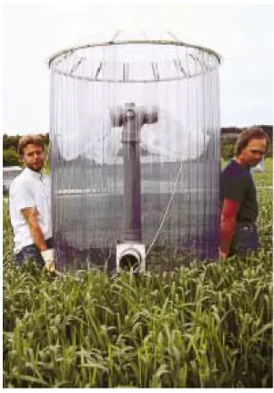
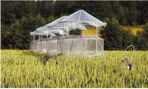
his report presents the final results of a series of experiments investigating the effects of ground-level ozone on plants, conducted since 1984 by the Swedish Environmental Re-search Institute (IVL) and the Botanical Institute at Göteborg University. Between 1985 and 1989, a field chamber experiment was carried out at Rörvik, some 40 km south of Göteborg, in which Norway spruces were grown at different ozone concentrations. This project was initiated by the power and district heating and forest products industries. Here we would therefore like to emphasize the important part played by Lars Lundgren, together with the late Hans Lundberg and the late Rolf Brännland, in developing this field of research. In 1987, experiments were started at Östads säteri, roughly 40 km north-east of Göteborg, to study the effects of ozone on field-grown agricultural crops. In 1990 the experiments on forest trees were moved to Östad. A larger-scale open-top chamber experiment was set up to study the effects of ozone, drought and phosphorus deficiency on Norway spruce, and this project continued up to and including 1996. 1994 saw the launch of the EC project ESPACE-Wheat, which studied the effects of elevated carbon dioxide concentrations combined with ozone and water availability on field-grown wheat over a period of three years. Between 1994 and 1996 research was also conducted into the effects of ozone on wild plants, and for this project, too, open-top chambers at Östad were used. In addition to this work, a series of experiments on pot-grown indicator plants for ozone have been undertaken at Östad since as early as 1988, in the framework of the Convention on Long-Range Transboundary Air Pollution (CLRTAP). An experiment to study the ozone sensitivity of birch was established in 1997.We would like to thank all the researchers, in Sweden and elsewhere, who have made important contributions to the experimental work carried on at Östad. In particular we would mention Dr D. Tingey, at the US EPA Corvallis, Prof. H. Sandemann, of GSF Munich, A. Berglen Eriksen, Senior Scientific Officer at the Phytotron, Oslo, Dr K. Ojanperä, at the Finnish Central Union of Agricultural Producers and Forest Owners, Jokioinen, and M. Werner MSc, of the Forestry Research Institute of Sweden.
Patrik Alströmer and Östads säteri played an active part in enabling the experiments to be conducted, by making available land, personnel and machinery, as well as contributing fi-nancially to the research relating to forest trees. We would like to express our special thanks to them for this. We are also greatly indebted to Cederroth International AB for the specially formulated nutrient solution used for the spruce saplings at Östad.
Finally, the authors wish to express their sincere thanks to Ulla Bertills at the Swedish Environmental Protection Agency for her enthusiastic involvement in their research, for her valuable comments and for the unstinting effort she has devoted to the preparation of this report.
GÖTEBORG, 19 APRIL 1999 THE OZONE RESEARCH GROUP
ATTHE SWEDISH ENVIRONMENTAL RESEARCH INSTITUTE (IVL) ANDTHE BOTANICAL INSTITUTE, GÖTEBORG UNIVERSITY
C
ONTENTS
E
XECUTIVESUMMARY6
1
O
ZONEANDTHEENVIRONMENT–
ABACKGROUND9
1.1 Introduction 9
1.2 Oxygen, ozone and life on earth 11
1.3 Ozone formation in the stratosphere and the troposphere 13
1.4 Ozone decreasing in the stratosphere, increasing in the troposphere 16
1.5 Ozone in environments with heavy traffic 19
2
I
NTERNATIONALANDNATIONALENVIRONMENTALOBJECTIVES21
2.1 Introduction 21
2.2 WHO and IMM guidelines on ozone – health effects 22
2.3 Effects of ozone on materials – a preliminary environmental objective 22
2.4 International control strategies 23
2.5 Critical levels of ozone 24
2.6 Swedish environmental objectives relating to ozone and ozone precursors 28
3
G
ROUND-
LEVELOZONEINS
WEDEN31
3.1 Introduction 31
3.2 Variation in ozone levels over Sweden 32
3.3 Ozone in mountain areas 33
3.4 Trends in ozone levels since the 19th century 33
4
E
FFECTSOFOZONEONAGRICULTURALCROPS37
4.1 Introduction 37
4.2 Experiments in Sweden 40
4.3 Effects on cereals 41
4.4 Effects on legumes 46
4.5 Effects on potato and tomato 47
4.6 Effects on oilseeds 48
4.7 Effects on forage crops 48
4.8 Exposure–effect relationships 49
4.8.1 Transport of ozone in the atmosphere 49
4.8.2 Transfer of ozone into the plant 50
4.9 The most ozone-sensitive crops 52
5
E
FFECTSOFOZONEONFORESTTREES55
5.1 Introduction 55
5.2 Effects on Scots pine 56
5.3 Effects on Norway spruce 56
5.3.1 Rörvik 1985–89 – Photosynthesis affected 57
5.3.2 The Ozone–Spruce project at Östad, 1992–96 – Growth affected 58
5.4 Östad Birch, 1997–99 66
5.5 Diagnosing the effects of ozone 70
5.6 Ozone combined with drought stress or phosphorus deficiency 71
5.7 Effects of ozone on older trees 73
5.8 Differing sensitivity to ozone 75
5.9 Gaps in current knowledge 76
5.9.1 How much ozone is taken up in different climates? 76
5.9.2 How ozone-sensitive are pine, oak, aspen and goat willow? 76
5.9.3 Sensitivity of seedlings, older trees and entire forests 77
5.9.4 Is it possible to develop diagnostic methods for field use? 77
5.10 Economic estimates of production losses 77
6
E
FFECTSOFOZONEONWILDPLANTS79
6.1 Introduction 79
6.2 Experiments in the Nordic countries 81
6.3 Effects on grasses and herbs 82
6.3.1 Visible injury and effects on growth 82
6.3.2 Ozone sensitivity in relation to systematics and growth strategy 82
6.3.3 The importance of competition 86
6.4 Effects on lichens and bryophytes 87
6.5 The most sensitive species 89
6.6 Important gaps in current knowledge 89
7
S
YNTHESISANDEVALUATION91
7.1 Effects of ozone on plants – current state of knowledge and research needs 91
7.2 Problems and prospects 93
8
S
OURCESOFFUNDING95
9
R
EFERENCES97
A
PPENDIXE
XECUTIVE
SUMMARY
O
zone in the lower atmosphere causes damage to plants and poses a threat to human health. It also damages materials and, furthermore, acts as a ‘greenhouse gas’, contributing to the greenhouse effect. Ozone forms, under the influence of sunlight, in air masses polluted with nitrogen oxides and hydrocar-bons. The single most important source of these ozone-forming compounds (ozone precursors) is transport, but industry and energy production also contribute. Emissions of ozone precursors have begun to fall in Europe and this trend may be expected to continue over the next ten years. Consequently, levels of ozone over the continent have probably also started to decrease. To some extent, ozone precursors disperse throughout the northern hemisphere, result-ing in an elevated background concentration of ozone. Some researchers take the view that this background level is rising, while others believe that it is more or less constant.There is now strong scientific evidence that production of sensitive agricul-tural crops, such as wheat and beans, is declining as a result of the ozone levels occurring across large areas of Europe. This is also the case in southern Sweden. Other plants, including various types of clover, spinach and tobacco, exhibit characteristic visible leaf injuries following ozone episodes, i.e. short periods of very high ozone concentrations. Such episodes chiefly occur in spring and summer in conjunction with high-pressure systems and sunny weather, when polluted air masses reach Sweden from more southerly areas of Europe. The main substances involved in ozone formation, which is a light-dependent pro-cess, are nitrogen oxides and certain volatile organic compounds. In southern Europe, ozone concentrations are locally greatly elevated from time to time during the warmer months of the year, and this can have very significant effects on certain crops, such as watermelon.
In various parts of the world, there is also evidence of ozone causing damage to forest trees. Here, though, the scientific case is not as compelling as in relation to agricultural crops, since most experimental studies have only involved young trees. The forests of the San Bernardino Mountains, south of Los Angeles, have suffered extensive ozone damage since the 1960s. Ponderosa (western yellow) pine especially has exhibited both significant visible injury symptoms and reduced production as a result of the very high ozone concentrations there. Ozone damage to forests has also been reported from the Mediterranean region.
In Spain, visible injury attributable to ozone has been observed in Aleppo pine, both in forest stands and in controlled experiments. In Sweden, detailed studies have been made of ozone’s effects on Norway spruce and silver birch. Following exposure to ozone, spruce needles that were more than two years old showed a decline in photosynthesis and chlorophyll concentrations. After four seasons, production was 5% lower in ozone-exposed spruce saplings than in a control involving preindustrial levels of ozone. Even cautious assumptions about the extent to which ground-level ozone interferes with the growth processes of forest stands suggest that present-day ozone concentrations will have an adverse effect of up to 10% on production in southern Swedish forests over an entire rotation. In a similar experiment on birch seedlings, ozone caused premature leaf-fall. The leaves were thus shed before their nitrogen content was returned to the stem, preventing the young trees from utilizing this nitrogen. In addition, after one season the birches exposed to ozone showed a decrease in the biomass of their roots. In the long term, high ozone concentrations probably depress production in birches. Reduced root growth may be assumed to restrict nutrient uptake, at any rate on less fertile soils, and earlier leaf-fall, combined with reduced with-drawal of nitrogen from the leaves to the stem, presumably further accentuates any nutrient deficiency.
Relatively little is known about the effects of ozone on wild plants. The enormous number of species involved is a major difficulty in this context. The experiments which have been carried out suggest that fast-growing species tend to be more susceptible to ozone than slow-growing ones. Quite a large number of wild species do not appear to be particularly sensitive to moderate increases in ozone concentrations. It should be borne in mind, though, that in the majority of ecosystems different herbs and grasses are in fierce competition with one another. This means that even fairly small differences in ozone sensitivity can result in shifts in the relative abundance of individual species if they are exposed to ozone.
The harmful effects of ground-level ozone on plants, health and materials are now an important driving force behind the international negotiations to reduce emissions of transboundary air pollutants in Europe. It is in this context that ‘critical levels’ of ozone have been formulated. These critical levels are currently based on the AOT40 concept (Accumulated exposure Over the Threshold 40 ppb ozone). AOT40 is calculated by adding together the amounts by which ozone concentrations exceed a level of 40 ppb. The purpose of the critical levels defined is to identify areas of Europe where ozone is having significant effects on vegetation. Critical ozone levels are currently exceeded in southern Sweden and, in the case of agricultural crops, to some extent in the north of the country as well.
There is now a shift in focus towards the amount of ozone taken up by plants, rather than simply the concentration in the ambient air. Sweden’s climate is favourable to ozone uptake. Long summer days and relatively high humidity mean that plants’ stomata (the tiny pores in their leaves) are open for long periods, resulting in comparatively high uptake of ozone. A given concentration may therefore have a more marked effect in this country than in an area with a drier climate and shorter days further south in Europe.
Over the next few years, research is likely to show that the exposure–response relationships that have been calculated on the basis of ozone concentrations overestimate the effects of ozone in southern Europe and underestimate its effects in the Nordic region. Preliminary estimates of ozone uptake in different parts of Europe point unequivocally in this direction.
Most of the studies presented in this report were carried out at Östads säteri. The experimental site can be seen at the bottom right of the picture. In the background, part of Lake Mjörn. Photograph: Svante Hultengren/Naturcentrum AB.
ppb – a unit to express ozone concentrations
Concentrations of ozone in air are usually expressed in either ppb or µg/m3. In this report we use the unit ppb, which expresses what is known as a partial pressure, or the proportion of the molecules in a parcel of air which are ozone molecules. The abbreviation ppb stands for ‘parts per billion’, i.e. the number of billionths (thousand millionths) of the air molecules present which consist of ozone.
The unit µg/m3 states the mass of ozone molecules present in a cubic metre of air, in micrograms (millionths of a gram). At normal pressure and temperature, the conversion factor is more or less exactly 2, i.e. 1 ppb O3 = 2 µg O3/m3, but to convert precisely from one unit to the other, pressure and temperature have to be taken into account. At high altitudes, the pressure is always lower and 1 ppb O3 corresponds to less than 2 µg/m3.
O
ZONE
AND
THE
ENVIRONMENT
– A BACKGROUND
Håkan Pleijel
S
UMMARYOzone is a factor behind a number of environmental problems. In the lower atmosphere, ozone formation is currently occurring as a result of emissions of nitrogen oxides and volatile organic compounds, and here the gas is affecting plants and human health and causing corrosion of materials. Ozone also contributes to the greenhouse effect. Periods of greatly increased ozone concentrations in the lower atmosphere are known as episodes. They chiefly occur in conjunction with stable high-pressure systems in summer, especially if air masses from the continent are involved. In areas with heavy traffic, ozone levels are locally lower, since ozone re-acts rapidly with the nitric oxide from vehicle emissions. The majority of the ozone in the atmosphere occurs in the ‘ozone layer’ of the stratosphere, at altitudes of about 10–40 km. Here, ozone levels are currently falling, owing to emissions of certain ozone-depleting substances, including CFCs (chlorofluorocarbons). This is a cause for serious concern, given that the stratospheric ozone layer protects life on earth from ultraviolet radiation.
1.1 Introduction
Ground-level ozone is a typical example of a regional pollutant. It forms when nitrogen oxides and volatile organic compounds undergo chemical reactions in the atmosphere under the influence of sunlight. It is no respecter of national boundaries and therefore constitutes an international problem. Ozone in the lower atmosphere has a number of different environmental effects. Apart from its effects on plants, which are dealt with in detail in this report, ozone at elevated concentrations also adversely affects human health (Bylin et al. 1996) and causes degradation of a variety of materials. Ozone is in addition a ‘green-house gas’, contributing to the green‘green-house effect.
In the United States, and especially in southern California, the problem of ozone attracted attention in the late 1940s. Emissions from road traffic were high even at that time and, in conjunction with the special climatic conditions
of the Los Angeles basin, they were giving rise to a mix of pollutants that is generally referred to as photochemical smog, or Los Angeles smog. The most important component of this smog is ozone, although it also includes a range of other pollutants, some of them particles which radically restrict visibility (figure 1.1). In Europe, too, high ozone levels are often associated with reduced visibility.
Figure 1.1. Photochemical smog in the San Bernardino Mountains in southern California. To the left is Paul Miller, a pioneer of research into the effects of ozone on forest trees. As early as the 1960s, he demonstrated the link between ozone and damage to ponderosa pine in the mountains south of Los Angeles. Photograph: Lena Skärby/IVL.
In Europe, extensive research collaboration relating to transboundary air pol-lutants and their chemistry has taken place since 1988 as part of the EUROTRAC project. In this forum, ozone formation has been seen as highly relevant in terms of effects on plants, human health, materials and climate (Borrell et al. 1997). Ozone-forming compounds (ozone precursors) and ground-level ozone feature very prominently in a protocol covering several different transboundary pollu-tants, currently being drawn up under the ECE Convention on Long-Range Transboundary Air Pollution. It is as part of the process of establishing a scientific basis for this protocol that ‘critical levels’ for the effects of ozone on plants have been identified. These critical levels are presented in chapter 2. In parallel with this work, the European Union (EU) is currently preparing a new directive on ground-level ozone. Control strategies will be linked to both the protocol and the directive, laying down how member states are to set about reducing ozone levels.
In several countries of Europe, the ozone issue is as serious a concern as acidification, for example. In this perspective, the health effects of ozone are a key factor, alongside its effects on plants. Compared with northern Europe, the countries of southern parts of the continent have less acid-sensitive soils and often appreciably higher ozone concentrations, and the balance of environmental concerns therefore differs. Nevertheless, ground-level ozone is a major envi-ronmental threat in Sweden, too, at least in the south of the country.
There are several common misunderstandings regarding ozone, its occur-rence and its environmental impacts. This is mainly because ozone forms in different ways, and has differing consequences for organisms on the earth’s sur-face, depending on where in the atmosphere it is found. To understand the issues involved, a historical, evolutionary approach may be helpful.
1.2 Oxygen, ozone and life on earth
When life on earth began, some 3500 million years ago, the atmosphere prob-ably contained no oxygen, or very little (Wayne 1985). Gradually, organisms capable of photosynthesis evolved, presumably a type of blue-green algae (cyanobacteria). Oxygen gas, or molecular oxygen (O2), is a by-product of tosynthesis. To begin with, virtually all the molecular oxygen generated by pho-tosynthesis was consumed by inorganic processes: the earth’s surface offered a plentiful supply of substances which it could oxidize, including sulphides and reduced (ferrous) iron. Around 2000 million years ago, there was little such material left to be oxidized, and from that point on oxygen gas began to accu-mulate in the atmosphere (Westbroek 1991). This had several important con-sequences, revolutionizing life on earth.
In many respects, oxygen is a poison. The gas itself and its by-products can oxidize molecules in the cells of organisms, which are then altered and cease to function. A significant part of the metabolism of an animal or plant is con-cerned with providing protection against the harmful effects of oxidizing agents. A key role in this protective system is played by substances known as antioxi-dants. Vitamin C (ascorbic acid) is one example of such a substance. Green plants in particular need to protect themselves against oxygen and other strong oxidants, since those substances are produced by photosynthesis. In certain re-spects, the life of a green plant is a balancing act between efficient production based on photosynthesis and a risk of self-poisoning by the by-products of that process. Some researchers believe that life on earth could not have come about if the atmosphere had contained oxygen gas from the outset. At the same time, the high concentration of oxygen in the atmosphere is the clearest sign that the earth is a planet supporting life.
Oxygen gas, then, can be dangerous because of its oxidizing capacity, but ozone is a far more powerful oxidant. Admittedly it occurs at much lower con-centrations, but it is more reactive, which is what makes it so harmful. Ozone is known to be capable of altering the chemical structures of fatty acids, modify-ing their chemical properties and possibly disturbmodify-ing their functionmodify-ing. Fatty acids are among the most important components of the membranes which round cells and cellular organelles and divide these structures from their sur-roundings. Ozone can also modify the chemical structures of proteins, which is a serious matter, since proteins of different kinds play a key part in the structure and metabolism of every organism. The differing functions of individual pro-teins are closely linked to their specific chemical structures.
Gradually, the earth’s organisms adapted to life in a world of high concentra-tions of molecular oxygen. Furthermore, some organisms began to exploit the considerable energy potential which lay in using oxygen gas to oxidize the or-ganic matter produced by photosynthesis. This process forms the basis for the supply of energy to the earth’s ecosystems at the present stage in the develop-ment of life, which began when the atmosphere started to contain large quanti-ties of oxygen gas (Goldsmith & Owen 1992). Animals, fungi and various other organisms are dependent on the oxygen produced by green plants, and the con-centration of molecular oxygen in the atmosphere thus needs to be fairly high; at present it is around 21%. It should be remembered, though, that 21% is not necessarily an optimum level for living organisms in every respect. It can be shown experimentally, for instance, that a lower oxygen concentration induces higher growth in plants, owing to a reduced oxidative stress. A higher concen-tration than that currently prevailing results in fires burning more vigorously, which results in oxygen being consumed. In other words, some sort of natural regulatory mechanism is in operation.
Had it not been for the change in the earth’s environment brought about by molecular oxygen, it is likely that life would have been a less prominent feature of this planet and would have consisted chiefly in mats of bacteria in the oceans. There are at least two reasons why oxygen was so important. Firstly, photosyn-thesis and respiration based on oxygen created conditions for far greater and more rapid conversion of energy than would otherwise have been possible. And secondly, the presence of oxygen in the atmosphere resulted in ozone begin-ning to form in the stratosphere. Ozone absorbs UV-B, an ultraviolet com-ponent of solar radiation which is very harmful to the majority of living organisms. Ozone formation therefore made it possible for life – previously concentrated in the protective oceans – to emerge onto the land. The ‘ozone layer’, which provides a shield against UV-B radiation, thus arose as an indirect
consequence of the accumulation of gaseous oxygen in the atmosphere. A major threat to the environment today is thinning of the stratospheric ozone layer at altitudes of around 15–40 km, so far primarily over the Antarctic, but to some extent also over other parts of the globe.
1.3 Ozone formation of ozone in the stratosphere
and the troposphere
The chemical basis for the formation of ozone (O3) is single atoms of oxygen (O). In the stratosphere, the latter can arise when short-wavelength and there-fore high-energy ultraviolet rays present in sunlight break down molecules of oxygen (O2):
Here, the symbol hn indicates that the reaction is dependent on light and the inequality above the arrow shows that the light must have a wavelength of less than 242 nm in order to drive the reaction. The shorter the wavelength, the higher the energy of the radiation. Ozone is then formed by single oxygen atoms combining with oxygen molecules:
The wavelengths in sunlight which are capable of driving reaction (1) do not reach the lowest layers of the atmosphere, and this process of ozone formation is therefore of no significance for the generation of ozone there. Solar radiation with a wavelength shorter than about 300 nm is absorbed by the ozone in the stratosphere. The layer of the atmosphere below it, extending to an altitude of about 10␣ km, is known as the troposphere. This is where the majority of impor-tant weather phenomena occur, and here ozone forms in a different way. In the troposphere, single atoms of oxygen are freed when nitrogen dioxide (NO2) is broken down into nitric oxide (NO) and an oxygen atom under the influence of sunlight:
Once again, the wavelengths in the sun’s radiation which drive the process are in the short-wave, ultraviolet region, but they are longer than those involved in reaction (1) and sufficient amounts of this radiation therefore reach the lower atmosphere. Reaction (2) occurs in the troposphere in the same way as in the stratosphere. NO + O l,410nm NO2+hv ➤ O3 O + O2 ➤ 2 O l,242nm O2+ hv ➤ (2) (1) (3)
S
TRATOSPHERICOZONEFORMATIONINBROADOUTLINEIn the stratosphere, short-wavelength, high-energy (ultraviolet) solar radiation can break down molecular oxygen, O2, into two single oxygen atoms, which are needed to form ozone, O3.
Ozone, too, can be broken down by sunlight. Normally, the two processes reach equilibrium at a fairly high ozone concentration.
When CFCs (chlorofluorocarbons) reach the stratosphere, they become chemically active as they are broken down by the short-wave radiation there and chlorine atoms, Cl•, are released. These chlorine atoms can participate repeatedly in the cycle of reactions by which ozone and single atoms of oxygen are transformed into molecular oxygen (O2). This reaction cycle reduces the ozone concentration in the stratosphere.
T
ROPOSPHERICOZONEFORMATIONINBROADOUTLINEAs in the stratosphere, the basis for ozone formation in the troposphere is single atoms of oxygen, O. Here, they are formed by longer-wavelength sun-light breaking down NO2 into NO and O.
NO reacts rapidly with ozone, which is consumed in the process. These reactions alone, therefore, do not result in really high ozone levels.
For there to be any net production of ozone, there has to be a reaction that competes with ozone for NO. At a certain stage in their decomposition in the atmosphere, volatile organic com-pounds (voc) can transform NO into NO2 without ozone being consumed.
Tropospheric ozone formation is complicated by two other important reac-tions. One is a comparatively rapid reaction between ozone and nitric oxide:
Reaction (4) consumes ozone formed by reaction (2). Reactions (2), (3) and (4) form a cycle which normally does not result in high ozone concentrations. For really high levels of ozone to arise, a further step is required. This is where vola-tile organic compounds come in. The majority of such substances are broken down in the atmosphere by a chain of reactions, some of which are dependent on light. If, to use the chemist’s terminology, we designate any organic com-pound of this kind as RH (the simplest of all hydrocarbons is methane, CH4, which in this terminology becomes CH3-H, with CH3 corresponding to R), the reaction steps we are most interested in here can be described as follows. In the atmosphere, hydrocarbons are primarily broken down by reactions with free radicals (usually short-lived, reactive particles). The most important of these in this context is the hydroxyl radical HO•. The dot after the chemical formula indicates that this particle has an unpaired electron, which is the main reason for its reactivity. Decomposition of hydrocarbons is initiated by the following reaction:
The free hydrocarbon radical R• then reacts rapidly with atmospheric oxygen to form a peroxy radical, RO2•. It is this radical which subsequently plays a part in ozone formation, in that it can oxidize NO to NO2 in competition with ozone:
Reaction (6) is important because NO is converted into NO2 without ozone being consumed as in reaction (4). Consequently, if suitable organic compounds are present in the air, nitrogen dioxide, which forms the basis for ozone forma-tion in the troposphere, can be regenerated time and time again. The radicals RO2• and RO• are short-lived reaction products formed during the decompo-sition of such organic compounds into carbon dioxide and water. (In the case of methane, the radicals concerned are CH3O2• and CH3O•, respectively.) It would not be unreasonable to say that organic compounds serve as the fuel and nitrogen oxides as the catalyst for tropospheric ozone formation. The organic compounds are oxidized and thus broken down or ‘burned’, primarily pro-ducing carbon dioxide and water. The nitrogen oxides, on the other hand, can be used repeatedly to form ozone without being consumed, which tallies with the definition of a catalyst. However, a nitrogen oxide molecule cannot participate indefinitely in ozone formation, since there are competing
NO2 + O2 NO + O3 ➤ R · + H2 O HO · + RH ➤ NO2 + RO· NO + RO2· ➤ (4) (5) (6)
processes which consume nitrogen oxides in the atmosphere. One of these is deposition onto vegetation and other surfaces. Another is chemical conversion of nitrogen oxides into other nitrogen compounds which play no part in the generation of ozone, chiefly nitric acid. Such reactions are more likely to occur in heavily polluted environments. The number of ozone molecules that can form per nitrogen oxide molecule emitted is therefore larger in comparatively clean environments, although the highest ozone concentrations are still found in the areas with the largest emissions of ozone precursors. Nevertheless, the higher rate of ozone formation per emitted nitrogen oxide molecule in cleaner environments is partly responsible for the wide geographical extent of the problem of ground-level ozone.
1.4 Ozone decreasing in the stratosphere,
increasing in the troposphere
More than 90% of the ozone in the atmosphere is to be found in the ‘ozone layer’ of the stratosphere. In recent decades, it has become clear that human beings have influenced the chemistry of the stratosphere in such a way that its ozone content has been depleted, a discovery that was rewarded in 1996 with the Nobel Prize for Chemistry. Certain air pollutants, above all chlorofluorocarbons (CFCs, or Freons), are able to cause changes in the stratosphere because they are highly stable, stability being one of the properties that have made such substances so useful for technical applications. As they do not degrade, they persist for a very long time in the atmosphere and are therefore eventually able to reach the strato-sphere. As noted earlier, this region of the atmosphere is exposed to shorter-wavelength and thus higher-energy radiation, in the face of which CFCs are no longer chemically stable. As they break down they release chlorine atoms, which can participate in catalytic reaction cycles that consume large amounts of ozone. These reactions are particularly efficient in association with certain types of stratospheric cloud. Such clouds only develop at very low temperatures, which primarily occur in the stratosphere over the Antarctic. This is an important part of the reason why the deepest ‘ozone hole’ is to be found in the stratosphere above the South Pole. Depletion of stratospheric ozone has also been observed over the planet as a whole, but not to the same extent.
In the troposphere, the opposite problem exists. Emissions of nitrogen ox-ides and volatile organic compounds, above all from transport, industry and energy production, have created the basic conditions for greatly increased tropo-spheric ozone concentrations in much of the industrialized world. True, a cer-tain amount of ozone was present in the troposphere even before the industrial revolution. Nitrogen oxides are formed by lightning discharges and forest fires
(Graedel & Crutzen 1993), for example, and volatile organic compounds that can play a part in ozone formation, chiefly terpenes and isoprene, are also emit-ted by plants (Simpson et al. 1995). However, in the course of the 20th century, background concentrations of ozone in Europe have increased by a factor of two to three from their preindustrial levels of 10–15 ppb (Borrell et al. 1997). In addition, what are known as ozone episodes occur. An episode is a relatively short period, anything from a few hours to a few days, of greatly elevated ozone concentrations, sometimes in excess of 100 ppb. In Sweden, ozone episodes usually occur when stable high-pressure systems, accompanied by strong sun-light and sun-light winds, move in across the country from the south, i.e. from the regions with major emission sources. As was noted earlier, sunlight – which is often strong during a period of high pressure – is important in ozone forma-tion. Since mixing of the air is restricted, ozone precursors – nitrogen oxides and volatile organic compounds – are not diluted and can reach high concen-trations. In Sweden, ozone episodes occur during most springs and summers, though to a very varying extent. Warmer, sunnier weather is normally accom-panied by more ozone episodes. High-pressure systems from the north do not usually produce ozone episodes, since they do not bring with them any appre-ciable quantities of ozone precursors.
Figure 1.3 shows how ozone levels at Rörvik, south of Göteborg, varied dur-ing the height of the summer of 1991. The values shown are 1-hour means. Fluctuations in the weather are clearly reflected in the ozone concentrations recorded: the diagram shows how spells of more or less unsettled low-pressure weather alternated with periods of high pressure. When low pressure prevailed, peak concentrations over each 24-hour period were not particularly high, per-haps reaching around 40 ppb, and levels were somewhat lower at night. At night, of course, no ozone is formed, since no light is available. High-pressure periods with more or less southerly winds were accompanied by ozone episodes. At such times, the ozone concentration rose to a diurnal maximum of almost 80 ppb, but frequently fell close to zero during the night-time. This considerable difference between day- and night-time levels is due to the fact that high-pressure systems are often associated with clear skies and little wind at night. Under such conditions, the ground surface cools down, since the thermal radi-ation which it emits to space is not reflected back by clouds, and a nocturnal inversion arises. The air nearest the ground ends up colder than the air above it, and vertical mixing in the lowest layer virtually ceases. All the ozone in the air closest to the ground is removed by deposition. Since mixing of the air is prac-tically non-existent, fresh ozone is not brought in from higher layers of the atmosphere, where, even at night, concentrations are usually quite high during episodes. Lows usually entail cloudy weather and it is generally windy enough,
Hourly mean O (ppb)3
albeit less so at night than during the day, to cause vertical mixing. For this reason, in such weather conditions, less marked vertical gradients of ozone con-centrations build up in the lowest part of the atmosphere.
Figure 1.3. Hourly mean concentrations of ozone (ppb) measured at Rörvik, some 40␣ km south of Göteborg, between 27 June and 12 August 1991. Redrawn from Pleijel et al. 1994c.
To sum up, most of the ozone in the atmosphere is to be found in the strato-sphere, where it ‘filters off ’ UV-B radiation which would harm organisms if it reached the earth’s surface. Stratospheric ozone levels are currently falling. In the troposphere, on the other hand, ozone concentrations are rising, owing to emissions of nitrogen oxides and volatile organic compounds. These diverging trends are illustrated by figure 1.4.
A subdivision of the ozone in the troposphere is also possible, into ground-level ozone and ozone in the free troposphere. The region of the atmosphere closest to the ground is known as the boundary, or mixing, layer. This layer is strongly influenced by mechanical turbulence, caused by friction between the air and the more or less rough ground surface, and by thermal turbulence, aris-ing from the fact that the surface and the air immediately above it are warmed by sunlight during the day. This heated air has a tendency to rise and thus to cause mixing. The depth of the boundary layer varies with the time of day and the season. Typical figures in summer may be 1000 m (about 10% of the entire troposphere) during the day and 100–200␣ m at night. Pollutants emitted at the ground surface disperse relatively quickly within the boundary layer.
Ground-level ozone is the ozone which occurs in this layer. Only high-altitude moun-tain areas reach into the free troposphere during the daytime.
There is no chemical difference between tropospheric and stratospheric ozone, but stratospheric ozone does not directly affect organisms on earth, since it is not inhaled by animals or taken up by plants. Between the troposphere and the strato-sphere there is a temperature boundary which greatly restricts transfers between these air masses. Sometimes, especially in early spring, some exchange does never-theless occur, especially at high latitudes. Since ozone concentrations are higher in the stratosphere, such an exchange involves a net input of ozone into the tropo-sphere. The dividing line between the boundary layer and the free troposphere is not at all as distinct, and exchanges between these two air masses occur regularly.
1.5 Ozone in environments with heavy traffic
The chemical reactions between primary air pollutants which are involved in ozone formation take some time and are regulated by sunlight, concentration changes, meteorology and other factors. This means that high levels of ozone can occur far away from emission sources and that the geographical link between sources and ozone formation is often fairly unclear. Nitrogen oxides released in one place may have an ozone-forming effect hundreds or thousands of kilometres away, by which time they will have been mixed with emissions from countless other sources. This explains the marked regional nature of the problem, and also means that emis-sions in other countries have a decisive impact on ozone concentrations in Swe-den. The ozone level at any particular location represents the sum of many small individual contributions from a very large number of sources. On the whole, there-fore, small-scale variations in ozone concentrations are limited. This is something
Altitude (km)
Ozone partial pressure (nbar)
Figure 1.4. Concentrations of ozone (expressed as partial pressure) at different altitudes. At about 10 km, there is a clear dividing line between the troposphere and the stratosphere. The measurements were made at Hohenpeissenberg in southern Germany. An upward trend in concentrations in the lower atmosphere and a downward trend in the stratosphere are clearly discernible.
of a problem for anyone wanting to study the effects of ozone. Concentration gra-dients are very useful for such purposes, but ozone concentrations vary on such a large geographical scale that, in order to find sites with substantially different ozone levels, very appreciable differences in climate and other natural conditions will also have to be taken into account.
There is one important exception to this rule, however, and one which also illus-trates the chemistry of ozone. In emissions from road traffic and combustion plants, the dominant nitrogen oxide is nitric oxide (NO). This means that the rapid reac-tion (4), in which ozone is consumed, is the first important reacreac-tion which comes into play when vehicle exhausts and flue-gas plumes mix with the ambient air. One consequence of this is that, in environments with heavy traffic, ozone levels are lower than in surrounding areas (Rodes & Holland 1981). This is in a sense a para-doxical state of affairs, in that transport emissions are at the same time the single most important cause of regional ozone formation, through reactions (2), (3) and (5). Because ozone concentrations are locally lower where traffic is heavy, ozone effects are in fact less marked in such areas, even though levels of several other primary pollutants emitted by vehicles are of course higher there. Figure 1.5 shows how the occurrence of visible ozone injury in an ozone-sensitive variety of clover varied with distance from the E6 motorway between Göteborg and Kungsbacka in the peak summer months of 1991 (Pleijel et al. 1994c). Noticeably less ozone dam-age was observed close to the road than 200␣ m away from it, where the degree of damage was at the level typical of rural areas of western Sweden during the period in question.
The local occurrence of lower ozone levels in the immediate vicinity of high road traffic emissions is the exception which proves the rule that concentra-tions of ground-level ozone do not vary appreciably, other than on a relatively large geographical scale.
No. of ozone-injur
ed leaves
Distance (m)
1 Aug 1991
12 Aug 1991, at harvest Figure 1.5.
Number of leaves of subterranean clover (Trifolium subterraneum ) injured by ozone, per pot, at different distances from the E6 north of Kungsbacka. The plants were exposed during the period covered by figure 1.3. From Pleijel et al. 1994c.
I
NTERNATIONAL
AND
NATIONAL
ENVIRONMENTAL
OBJECTIVES
Håkan Pleijel
S
UMMARYAt both the national and the international level, environmental objectives and limit values relating to ozone have been adopted. The UN agency WHO and the Swedish Institute of Environmental Medicine (IMM) have collated scientific data on levels of ozone that could be harmful to human health. WHO has proposed a level of 60 ppb for effects of this type, while the IMM wishes to set a more stringent limit of 40 ppb. In response to rising concen-trations of ground-level ozone in Europe, the ECE has developed critical
levels of ozone with regard to its effects on vegetation. These are being used to
design effects-based control strategies to reduce emissions of ozone precur-sors under the ECE Convention on Long-Range Transboundary Air Pollu-tion and within the EU. At present, critical levels are based on an exposure index known as AOT40, which refers to the accumulated exposure to ozone in excess of 40 ppb. Regarding the effects of ozone on materials, European experts have discussed using 20 ppb for the time being as a kind of critical level which should not be exceeded. In Sweden, official environmental objec-tives exist with regard to emissions of nitrogen oxides and hydrocarbons, the pollutants which result in ozone formation.
2.1 Introduction
As was mentioned in chapter 1, ozone is a contributory factor behind several types of environmental impact, both health effects and effects on plants and materials. As a result, various national and international bodies have formu-lated environmental objectives and limit values with respect to ground-level ozone and ozone precursors. The main bulk of this report is concerned with ozone’s effects on plants, and it may therefore be appropriate here also to touch on its significance for health and materials.
2.2 WHO and IMM guidelines on ozone – health effects
The World Health Organization (WHO), a specialized agency of the UN, issues guidelines on, among other things, the levels of air pollutants that are regarded as harmful to human health. As noted in chapter 1, ozone is a powerful oxidant. It has a relatively low solubility in water and is therefore drawn deep into the lungs when inhaled. After only fairly brief exposure, ozone produces inflamma-tory reactions in the respirainflamma-tory tract. These abate when exposure ceases. In experiments, such effects have been observed at ozone levels down to around 80 ppb. Ozone impairs lung capacity and reduces resistance to bacterial and viral infections. The first of these effects is particularly serious for individuals who already have impaired lung function, such as asthma sufferers. Irritation of the eyes is another common effect of elevated, but currently occurring ozone concentrations. People who spend a lot of time outdoors and are highly active physically are particularly at risk. This category includes those who engage in sports, but generally children also have a tendency to be especially vulnerable, since they are often in the open air and move about a great deal. Epidemiologi-cal research has shown that high ozone levels co-vary with hospital admissions for lung complaints. There are also studies suggesting that ozone may increase the risk of cancer, although this risk has not been adequately assessed. On the basis of the ‘lowest observed effects’ level, WHO has formulated a guide value of 60␣ ppb ozone as the maximum 8-hour mean (WHO 1995). At the same time, WHO stresses that this level probably does not represent any margin of safety for the most sensitive sections of the population with regard to certain types of acute health effect. The Swedish Institute of Environmental Medicine (IMM) has recommended a low-risk level of a 1-hour mean of 40 ppb ozone, as an upper limit for human exposure (Bylin et al. 1996). This was calculated using a safety factor of 2 in relation to the lowest observed effects level.2.3 Effects of ozone on materials – a preliminary
environmental objective
Ozone has long been known to affect polymers, i.e. molecules of the type found in the majority of fibres. The polymers affected are those containing carbon atoms with double bonds, which include many natural fibre materials, such as natural rubber, cotton and cellulose. Best known is ozone’s effect on rubber, and in the 1950s this material was used as a simple means of measuring atmos-pheric levels of the pollutant. Ozone causes rubber to crack, and the depth of the cracks that appear over a given time is a measure of how high the ozone concentration has been. This method proved to have a good degree of
preci-sion. One of the sectors interested in ozone levels back in the 1950s was manu-facturers of car tyres, which are made from rubber.
Ozone also affects a range of other materials, resulting in costs to society and damage to cultural assets. For example, it shortens the lifetimes of textiles, paints and other pigments (e.g. on museum exhibits). Unlike the effects of ozone on human health and plants, the scale of the damage it causes to materials is pri-marily determined by the long-term average concentration of the gas. In prin-ciple, all concentrations have some effect. Nevertheless, European experts have discussed setting a critical level for ozone with respect to effects on materials at an annual mean of 20 ppb. At present, this value is exceeded virtually through-out Europe. Current estimates of the financial cost of ozone’s effects on ma-terials are very uncertain, but the sums involved could be considerable.
The biggest concentrations of materials that could be damaged by ozone are to be found in major towns. As indicated in chapter 1, ozone levels are usually somewhat lower there than in the surrounding countryside, since ozone is con-sumed locally by vehicle emissions of nitric oxide (NO). This creates a paradox: if a town manages to cut nitrogen oxide emissions locally, ozone levels will rise and with them the risk of damage to materials, or at least they will do so unless the same emission reduction is achieved over a wide geographical area. This underlines the need for large-scale strategies to reduce ozone loads in Europe.
2.4 International control strategies
In recent decades, various agencies have endeavoured to introduce measures to curb the effects of ozone. At the international level, the ECE Convention on Long-Range Transboundary Air Pollution has been most important. The ECE (the United Nations Economic Commission for Europe) played a significant role in promoting international dialogue in Europe during the cold war. One of its key spheres of activity was transboundary air pollution. Since this organiza-tion included the Warsaw Pact countries among its members, air polluorganiza-tion could provide a pretext for discussing other important political issues as well. Under the ECE Convention, several international protocols to control a range of air pollutants have been signed. At present, the final touches are being put to a protocol covering, among other things, nitrogen pollutants and volatile organic compounds (VOCs). An important driving force behind this ‘multi-pollutant/ multi-effect protocol’ has been the effects of ground-level ozone, both effects on human health and damage to vegetation. ‘Critical levels’ of ozone, described in more detail in the next section, have formed an important part of the scien-tific basis for the protocol.
In recent years, the European Union has emerged as an increasingly power-ful player in the arena of transboundary air pollution. It is currently drawing up an Acidification Strategy and an Ozone Strategy, which will guide future EU efforts in this field. A crucial consideration in the EU’s Ozone Strategy is cost-effectiveness. The emission reductions that can be achieved at low cost are al-ready being implemented or have at least been decided on in a good number of countries, and further cuts will prove more expensive. To secure acceptance and legitimacy for the costs involved among those who will have to meet them – companies, states (taxpayers) and consumers – it is important to ensure that any action is as cost-effective as possible. In other words, it must be possible to show that the measures decided on are the ones that will yield the greatest en-vironmental benefits per unit of currency invested. The new control strategies are therefore effects-based, which was not the case with the earliest protocols under the ECE Convention.
The EU’s new directive and strategy on ozone will be based chiefly on the ECE-defined critical levels for the effects of ozone on plants and on WHO’s guidelines with regard to health. To a large extent, the calculations underlying the cost-effective, effects-based control strategies currently being discussed within the ECE and the EU are being performed by IIASA, an international centre for systems studies near Vienna.
2.5 Critical levels of ozone
The process of establishing critical levels of ozone began in 1988, when a work-shop was held in Bad Harzburg in Germany on the initiative of the ECE. At that meeting, preliminary critical concentrations with regard to effects on plants were calculated for a number of gaseous air pollutants (Guderian 1988). These efforts were guided by an older tradition in toxicology which relied on mean concentrations over a given period of time. In this early work, ozone was less prominent compared with other pollutants, chiefly sulphur dioxide and nitro-gen oxides, than it is today.
To build on the results from Bad Harzburg, a similar meeting was held at Egham near London in spring 1992, and once again a range of gaseous air pol-lutants were dealt with (Ashmore & Wilson 1994). At that workshop, it became increasingly clear that, in quantitative terms, ozone was the dominant gaseous air pollutant in Europe with regard to effects on plants, although sulphur diox-ide will probably continue to have significant effects in parts of eastern Europe for some time to come.
Another very important outcome of the Egham workshop was the launch of a new approach to describing exposure to ozone. It was demonstrated that the
observed effects of ozone showed closer agreement with the aggregate exceedance of a given threshold value than with the mean concentration figures tradition-ally used. This new approach was not fully developed until the next European workshop on critical levels, held in Berne in autumn 1993, which dealt only with ozone (Fuhrer & Achermann 1994). A collation of the results of European experiments on ozone exposure of field-grown wheat revealed a very high cor-relation with the exposure indices AOT40 and AOT30. AOT stands for ‘Accu-mulated exposure Over Threshold’, i.e. the aggregate exceedance of a stated ozone concentration over a given period. Assuming ozone concentrations are expressed in ppb – parts per billion (i.e. per thousand million) of the total number of air molecules – the unit used for the AOT index is ppb-hours. The main reason for choosing AOT40, i.e. for setting the ‘threshold’ at 40 ppb, was that a lower thresh-old would have been close to the background concentrations of ozone occur-ring in ambient air throughout the northern hemisphere. AOT40 is a measure which clearly reflects the extent to which ozone concentrations are elevated as a result of anthropogenic emissions of ozone precursors. It is the first step to-wards a dose measure indicating ozone doses harmful to plants. AOT40 does not directly reflect plant uptake of ozone, being calculated solely on the basis of concentrations in air. Efforts to develop an uptake-based exposure index for ozone are now under way, but a generally accepted method for this purpose has yet to be established.
C
ALCULATING AOT40AOT40 is calculated as follows. Assume that the following hourly mean concentrations of ozone have been recorded over seven hours: 35, 38, 40, 41, 42, 45 and 50 ppb. The first three values do not contribute to the exposure index, since they do not exceed 40 ppb by at least 1 ppb. Only the last four values contribute to AOT40. The AOT40 value is thus: (41-40) + (42-(41-40) + (45-(41-40) + (50-(41-40) = 1 + 2 + 5 + 10 = 18 ppb-hours. For agricultural crops, differences are aggregated over a three-month period (May–July), while for forests a six-month period (April–September) is used. Since plants chiefly take up ozone in daylight, AOT40 is calculated on the basis of values for the hours between sunrise and sunset.
AOT40 values have been used to develop relationships between exposure and response in plants. As indicated above, the best results have been obtained with regard to effects on wheat yields. Figure 2.1, based on a large body of data from five European countries, shows what such relationships may look like. A more detailed relationship for the Nordic countries will be presented in chapter 5.
Relativ
e yield (%)
AOT30 (ppb-hours) AOT40 (ppb-hours)
Figure 2.1. Relationships between yields of wheat (as a percentage of the yield when AOT30 or AOT40 = 0 in the experiments) and AOT30 and AOT40, respectively, in experiments carried out in five European countries. The diagrams show linear regressions, with the 99% confidence limits.
At the following ECE workshop, in Kuopio in 1996, it was agreed that, for the time being, the critical levels shown in table 2.1 were to apply (Kärenlampi & Skärby 1996).
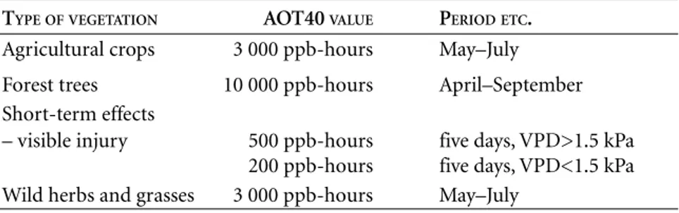
Tabell 2.1. Critical levels of ozone defined at the Kuopio workshop in 1996. From Kärenlampi & Skärby (1996). VPD = vapour pressure deficit, a measure of how dry the air is.
TYPEOFVEGETATION AOT40 VALUE PERIODETC.
Agricultural crops 3 000 ppb-hours May–July Forest trees 10 000 ppb-hours April–September Short-term effects
– visible injury 500 ppb-hours five days, VPD>1.5 kPa 200 ppb-hours five days, VPD<1.5 kPa Wild herbs and grasses 3 000 ppb-hours May–July
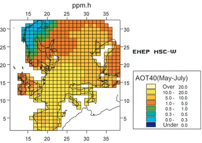
Figure 2.2 shows how ozone levels, expressed as AOT40, varied across Europe in May–July over the period 1989–94 (Simpson et al. 1998). The diagram is based on modelled values, which are in close agreement with those obtained from measurements.
Figure 2.2. Ozone exposure in Europe, expressed as AOT40 (ppm-hours; 1 ppm = 1000 ppb) over the period May to July, modelled values for 1989–94. Map made available by David Simpson at the Norwegian Meteorological Institute (DNMI).
(May-July)
Over
Under
In scientific terms, the most certain of the critical ozone levels calculated so far is the figure for agricultural crops, which is based on yield reductions in wheat. A relatively large body of data is available, and the results are consistent. The critical level for forest trees is more uncertain. It is based on data for beech, which the information available indicated was more sensitive to ozone than spruce, for example. The AOT40 values for short-term exposure refer to the occurrence of visible injuries to leaves during ozone episodes, and are based on experiments involving clover. The abbreviation VPD in table 2.1 stands for vapour pressure deficit, which is a measure of the dryness of the air. Basically, it indicates how strongly the air tends to draw water from plants. At high VPDs, plants close their stomata, the tiny pores in their leaves which regulate their exchange of gases with the atmosphere. This reduces transpiration, i.e. the loss of water vapour to the surrounding air. Another consequence of closed stomata is that plants take up smaller amounts of gaseous air pollutants, such as ozone, and exposure therefore has to be higher to have the same effect. Broadly speaking, the two levels for short-term effects reflect the difference in climate between the warmer southern and eastern parts of Europe, with dry summers, and the dam-per, cooler regions of northern and western Europe. Although high VPDs do sometimes occur in Sweden in summer, the relevant AOT40 value here is by and large the lower one. The value for wild herbs and grasses is provisional. It is
based primarily on outline experiments on large numbers of species, which have indicated that the most sensitive species probably have roughly the same sensitivity as the most sensitive crops. The majority of wild plants are probably less sensitive.
All the values presented in the table above are what are known as Level I critical levels, which means that they are used to estimate the risk of production losses or visible injury in different groups of plants, regardless of all the factors which may locally modify the effects of ozone. Such factors include genetic vari-ation within and between species, the developmental stage at which plants are exposed, the presence of pest organisms and other pollutants, and a range of climatic factors (wind, light, soil moisture, atmospheric humidity, temperature) which affect ozone uptake. Level I values are not intended as a basis for esti-mates of actual production losses or other effects, but simply indicate in which areas there is a risk of significant ozone damage to vegetation. The focus is now shifting towards developing Level II values, which are intended to be used to estimate the scale of effects in ecosystems. To do that, the factors mentioned have to be taken into account. Only limited progress has been made in this direction as yet, but this is likely to be a key concern of ozone research in Europe over the next few years.
2.6 Swedish environmental objectives relating to ozone
and ozone precursors
The Swedish Government recently submitted a bill to Parliament entitled ‘Swed-ish Environmental Objectives. Environmental Policy for a Sustainable Sweden’ (Government Bill 1997/98:145). The Government’s overall goal for efforts in the environmental field is to be able to hand over to the next generation a soci-ety in which the country’s major environmental problems have been solved. In addition, at the international level, Sweden should be a driving force and pioneer of ecologically sustainable development.
To achieve these aims, the Government has proposed that a new structure for setting and implementing environmental objectives should be established. A limited number of national environmental quality objectives will be adopted by Parliament, indicating what state of the environment is to be achieved on a time-scale of one generation. The Government will have a responsibility to en-sure that, where necessary to achieve these objectives, more specific goals are defined. The latter will then form the basis for the definition of aims and strat-egies in different sectors of society and at different levels. Since this is a new approach, the Government has set up a parliamentary advisory committee to keep the process under review, in collaboration with the government agencies
concerned. In practice, several authorities (the Environmental Protection Agency, the Board of Agriculture, the Board of Forestry etc.) have already embarked on this process. The Government’s assessment is that environmental quality objec-tives, together with the new Environmental Code (Government Bill 1997/98:45), offer greater scope for a decentralization of environmental protection. Oppor-tunities for and interest in taking independent initiatives to secure a better environment will increase, not least in the business sector.
The problem of ground-level ozone is addressed under one of 15 environ-mental quality objectives which are proposed, namely Clean air. The objective proposed by the Government is that ‘the air should be so clean that no damage is caused to human health or to animals, plants or cultural assets’. Existing air quality problems in urban areas of Sweden are chiefly the result of Swedish emissions, with transport the most important source of all; locally, small-scale burning of wood may also be a major source. Problems relating to ground-level ozone in Sweden, however, are for the most part attributable to emissions in other countries, primarily the United Kingdom and Germany. Sweden is only the third most important of the countries contributing to the ozone levels oc-curring within its borders. It should not be forgotten, though, that Sweden also exports ozone precursors – nitrogen oxides and hydrocarbons – to its neigh-bours, inter alia from the above-mentioned urban areas.
As far as ground-level ozone is concerned, the environmental quality objec-tive proposed means that concentrations should not exceed the limit/guide val-ues that have been established to prevent harm to human health, animals, plants, cultural assets and materials. Emissions of nitrogen oxides need to be reduced, and under the quality objective Natural acidification only the Government has said that nitrogen oxide emissions from the transport sector in Sweden should have fallen by at least 40% by the year 2005, compared with 1995 levels. The Government’s assessment is that this objective should be supplemented with targets relating to volatile organic compounds and that ‘additional more spe-cific targets may need to be developed’. In its Transport Policy Bill (1997/98:56), the Government put forward the view that transport emissions of VOCs in Sweden should be reduced by at least 60% by 2005, compared with 1995 levels. It has been decided that the transport sector’s emissions of nitrogen oxides are to be cut by 40% and those of VOCs by 60% between 1995 and 2005. These reductions are relevant to the environmental quality objective Clean air. To at-tain this objective, action must also be taken to reduce emissions from small-scale wood burning and from industrial plants and district heating and power stations. To achieve the quality objective with respect to ground-level ozone, further emission cuts will be necessary both in Sweden and in other European
countries. Negotiations on what additional commitments different countries need to make are being conducted under the UN ECE Convention on Long-Range Transboundary Air Pollution (CLRTAP) and within the EU. Finally, fur-ther action in the transport sector is of great importance. Legislation on vehicle emissions lays down maximum permitted releases of different pollutants from road traffic. In the context of the Environmentally Sound Transport System (MaTs) project, the transport sector has set targets of a 70% reduction of VOC emissions by the year 2005 and an 85% reduction by 2020, compared with 1988.
Chapter 3
G
ROUND
-
LEVEL
OZONE
IN
S
WEDEN
Karin Kindbom and Håkan Pleijel
S
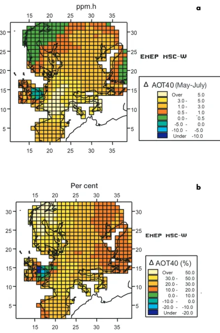
UMMARYAs part of Sweden’s environmental monitoring programme, ozone con-centrations are measured continuously at a number of sites around the country. These measurements show that critical levels for damage to agri-cultural crops and forests are exceeded in southern Sweden, but only to a very limited extent (crops) or not at all (forests) in the north of the coun-try. By the year 2010, emissions of ozone precursors in Europe are ex-pected to have fallen. This will result in a reduced exceedance of critical ozone levels, particularly over certain parts of the continent. In Sweden, too, the ozone load will decrease, but the critical level for crops is expected to be exceeded even after 2010.
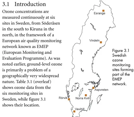
3.1 Introduction
Ozone concentrations are measured continuously at six sites in Sweden, from Söderåsen in the south to Kiruna in the north, in the framework of a European air quality monitoring network known as EMEP (European Monitoring and Evaluation Programme). As was noted earlier, ground-level ozone is primarily a problem of a geographically very widespread nature. Table 3.1 (overleaf) shows ozone data from the six monitoring sites in Sweden, while figure 3.1 shows their location.Figure 3.1 Swedish ozone monitoring sites forming part of the EMEP network.
3.2 Variation in ozone levels over Sweden
As table 3.1 shows, long-term mean concentrations of ozone do not differ dra-matically between the south and the north of Sweden. When it comes to AOT40 values and maximum hourly means, however, the differences are very pro-nounced. Appreciably lower values are recorded for these exposure measures at the two northern sites of Vindeln and Esrange. This is because these areas are affected by far fewer ozone episodes, and those that do affect them have usually largely abated by the time they reach this far north. On the other hand, there is a more marked spring peak in ozone concentrations at these two sites, and it occurs earlier there, normally in April. There may be various reasons for this. One possible explanation is that volatile organic compounds accumulate in the atmosphere during the polar winter, since their decomposition is a light-dependent process. When strong sunlight returns after the spring equinox, these pollutants give rise to ozone formation. Another conceivable explanation is that ozone from the stratosphere is mixed into the troposphere in the early spring Table 3.1. Mean ozone concentrations for April–September (24-hour, ppb), AOT40 values for the period May–July/April–September (ppb-hours), and highest recorded hourly mean concentrations of ozone (ppb) at six Swedish EMEP monitoring stations. AOT values exceeding agreed critical levels (table 2.1) are printed in bold.
MEAN AOT40 AOT40 MAXIMUM
CONCENTRATION MAY–JULY APRIL–SEPTEMBER HOURLYMEAN
APRIL–SEPTEMBER CROPS FOREST CONCENTRATION
1994 Vavihill 36 10 215 14 512 100 Norra Kvill 39 13 781 19 758 98 Rörvik 38 11 113 17 139 88 Aspvreten 34 8 166 10 320 78 Vindeln 29 2 178 4 858 78 Esrange 36 3 285 9 053 80 1995 Vavihill 36 7 143 12 535 103 Norra Kvill 35 6 507 9 820 86 Rörvik 34 5 892 10 062 82 Aspvreten 34 7 742 11 229 72 Vindeln 29 2 147 3 195 64 Esrange 34 3 843 7 000 61 1996 Vavihill 37 5 793 16 880 105 Norra Kvill 36 4 520 13 632 91 Rörvik 35 4 668 12 026 98 Aspvreten 36 7 081 15 570 86 Vindeln 30 2 477 5 285 69 Esrange 34 1 878 4 848 62
and that this occurs to a particularly large degree in the north. Both these factors probably contribute to the pattern observed. The fairly high altitude of the Esrange measuring station is presumably also partly responsible for the com-paratively high average ozone levels recorded there.
A collation of ozone data for northern and western Europe from 1989, which was a year with relatively high ozone concentrations, shows that AOT40 for the period April–September varied from about 1500 ppb-hours at Ny Ålesund in Svalbard to 20␣ 000–40␣ 000 ppb-hours in parts of continental Europe (Beck & Grennfelt 1994). The highest values were recorded in mountain regions.
3.3 Ozone in mountain areas
Within a given region, the highest mean concentrations of ozone are usually found at high altitudes. This has probably always been the case (Borrell et al. 1997). In addition, ozone levels follow a different diurnal pattern in mountain areas: they remain almost constant between day and night, and night-time con-centrations are very high compared with those in low-lying regions. This is very much the case in the Alps, for example, and the same phenomenon has been observed on Åreskutan in the Swedish mountain range (Bazhanov & Rodhe 1996). As indicated earlier (section 1.4), monitoring sites at high altitudes in mountain regions (above approx. 1000 m) are often situated within the free troposphere, the part of the troposphere that is above the boundary layer and is therefore little affected by local emissions. The fact that they are in the free troposphere also means that ozone concentrations there are affected very little by deposition, since there are only small areas of land and vegetation at such high altitudes onto which ozone can be deposited. This is an important part of the explanation for the high ozone levels recorded at night at high-altitude sta-tions in mountain areas. Down below, in the boundary layer, ozone is removed at the ground surface by deposition during the night. Since such a small pro-portion of the land mass is situated above the boundary layer, the deposition occurring there is of less significance.
3.4 Trends in ozone levels since the 19th century
Ozone was discovered in the middle of the 19th century by a chemist called Schönbein, who also developed a method of measuring the gas, known as Schönbein paper. This paper was exposed for a day and the ozone concentra-tion could then be read off against a colour scale. Measurements performed with Schönbein paper in the 19th century – in Paris, the Pyrenees and northern Italy, for instance – suggest that background levels at that time were about 10 ppb (Volz & Kley 1988; Anfossi et al. 1991), but there are also early studies