Analysis of hailstones from northeastern Colorado

TA1

e~

C£e-1oa-38

~.2-ANALYSIS OF HAILSTONES from

Northeastern Colorado, 1962

by

Ron R. Robinson

May, 1963

from

Northeastern Colorado, 196 2

By

Ron R. Robinson

Preliminary Progress Report - For the Record {Data from this report are to be extracted for publication)

Civil Engineering Section Colorado State University

Fort Collins, Colorado May 1963

This work was supported by the National Science Foundation Grant NSF G-23706

Chapter I II III IV INTRODUCTION . . PROCEDURES . . . . A. Laboratory • • . . . . 1. Slicing process . . . . 2. Photographing hailstone slices . 3. Density measurements •

B. Field work . . . .. . . ..

1. Collecting hailstones .

.

.

. .

.

2. Slicing hailstones . . 3. Photographing hailstones . 4. Density measurements . DATA ANALYSIS . . . . A. Hailstone parameters . 1. Size . . . . 2. Shape . . . 3, Density . . . . 4. Ice crystal ratio

5. Growth rings . . . 6. Embryo diameter . . 7. Amount of data . . 8. Accuracy of data B. Radar data

RESULTS . . . . . • . . .

A. Mean hailstone properties 1. Density . . . .

2. Size . . . . 3. Ice crystal ratio

4. Growth rings . . 5. Embryo diameter . 6. Hailstone shape . 7. Embryo shape . . . . 8. Type of embryo . 9. Summary . . . .

B. Hailstone parameter means and variability by months . . 1. Density . . . • • . 2. Ice crystal ratio . . . .

3, Size . . . . 4. Embryo diameter .

C. Hailstone parameter means by geographic areas i Page 1 1 1 1 2 3 3 3 4 4 4 4 4 5 5 5 5 6 6 6 7 7 8 8 8 8 8 9 9 9 10 10 10 11 12 12 12 12 12

Chapter V VI VII VIII IX X SIMPLE CORRELATIONS . . . • . . . • . A. Total analyzed hailstones . . . .

Page 13 13 B. Hailstone parameter correlations by months 14 C. Hailstone parameter correlations by geographic areas . 17 PREDICTION OF DENSITY FROM OTHER HAILSTONE

PARAMETERS . . . . A. Prediction equations by months

B. Prediction equations by quadrants ANALYSIS OF VARIANCE

A. F tests . . . . B. Students' "t" tests

SIMPLE CORRELATIONS BETWEEN HAILSTONE PARAMETERS AND THUNDERSTORM PARAMETERS SUMMARY AND CONCLUSIONS. . . . • . REFERENCES . . . . • . . . • . . . . • . . ii 20 20 20 21 21 21 21 22 24

Figure 1 2 3 4 5 6 7 8 9 10 Photo box . Density kit Title

Density correction graph Map of four geographic areas

Scatter diagram of hailstone diameter vs c_oud tops Scatter diagram of hailstone diameter vs Z .

max Scatter diagram of hailstone diameter vs tilt . . . Scatter diagram of hailstone density vs clo d tops Scatter diagram of hailstone density vs Z

max Scatter diagram of hailstone density vs tilt . . .

iii Page 25 26 27 28 29 30 31 32 33 34

Table 1 2 3 4 5 6 7 8 9 10 11 12 13 14 15

Frequency of occurrence of small, medium, and large

hailstones . . . .

Frequency of occurrence of small and large ice crystal ratios ~

Frequency of occurrence of different shapes of hailstones . . .

Frequency of occurrence of embryo shapes for 407 hailstones .

Mean hailstone parameters (x), standard deviations (s),

and number of samples (N) . . . .

Mean hailstone parameter (x), standard deviations (s), and

number of samples by quadrants from Sterling, Colorado Simple correlation coefficients for all ( 25 7) hailstones . .

Simple correlation coefficients for May ( 27) hailstones Simple correlation coefficients for June (50) hailstones Simple correlation coefficients for July ( 180) hails ones Simple correlation coefficients for 64 hailstones in area I

Simple correlations coefficients for 6 9 hailstones in area II

Simple correlation coefficients for 81 hailstones in area III

Simple correlation coefficients for 34 hailstones in area IV Simple correlation coefficients between hailstone parameters

and thunderstorm parameters . . . .

iv Page 8 9 10 10 11 13 14 15 15 16 17 18 18 19 22

Cold box

Cooperators · Density

Dry growth

rings

Ice crystal

ratio Large ice crystals

Larg~

hail-stones

Small portable refrigerator

People who collect and report hail

Ratio of weight of ice to the same volume of water,

diemen-sionless

Rings of ice made up of small ice crystals

Volume of small ice crystals in a hailstone divided by the volume

of large ice crystals in the hailstone

O. 3 to oo cm in length dimensions

Hailstones with diameter > 3 cm

Max Z values Max reflectivity Medium

hail-stones Hailstones with diameter from 1. 5

+

to 3 cm

Small ice

crystal ratio A ratio from O. O to 1 Small ice

crystal 0. 0 to O. 3 cm in length dimension

Large ice

crystal ratios A ratio from i to

ro

Tilt Angle of thunderstorm core from the vertical Wet growth

rings Ice rings made up of large ice crystals

A large number of hailstones were collected in Northeastern Colorado during the summer of 196 2. Certain measurements were made on these stones for the purpose of determining their physical characteristics. Measurements were made of the following:

Density,

Ratio of small ice crystals to large ice crystals in individual hailstones,

Number of wet and dry growth rings,

Diameter of the hailstone or shape of stones,

Size of the embryo, and Shape of the embryo.

The mean, standard deviation, variance and coefficient of variation of

each of these parameters was computed for each sample. Simple correlation coefficients were computed between these parameters for individual stones.

The data were analyzed to determine seasonal and geographical variation.

The physical properties of hailstones were compared to the physical properties (Z values, cloud tops, tilt of core) of the storms from which they fell by

computation of simple correlation coefficients.

II. PROCEDURES

A. Laboratory

1. Slicing process - while the slicing of hailstones for photographing is a tedious and exacting operation, with some practice it is possible to slice and photograph four stones per hour.

For slicing a hailstone an apparatus was used which contained two hot wires attached to an inclined plane ( 1),:, . These two wires could be adjusted to cut any thickness desired. The hailstone was frozen to a brass cart, which was

rolled down the inclined plane. The hot wires made contact with the hailstone,

and were adjusted to cut a hail slice three millimeters thick. The hailstone slice

was then polished on a damp chamois to a final thickness of one millimeter. The slice was then ready to be photographed for air bubble structure.

2. Photographing hailstone slices - Photographing a hailstone slice must be done at

o°

C or colder. To accomplish this, a photobox was mounted

in a refrigerator. The photobox contains its own light source, cross-polarized

lenses, and a roleflex camera mounted in the top. For black and white pictures the film used was Pan-X-125. In taking a picture of the air bubble structure,

only one polarized lens was used. The hail slice (one millimeter thick) was

placed in the photobox, .and a time exposure of five seconds was taken. The hail slice was then removed and further polished to a thickness of one tenth of a millimeter. Again the hailstone was placed in the photobox with two polarized

lenses crossed. For a picture of the crystal structure of the hail slice, the time exposure was eighteen seconds.

The cross polarized lenses let only the refracted light from the crystals pass through to the camera, thus giving a picture of the crystal structure to the hail slice.

For taking color photographs of the crystal structure of hailstone slices

a 35 mm single lens reflex camera was used which contained a bellows attach-ment with a magnification of 2. 7. The bellows attachment made it possible to take detailed pictures of small hailstone slices. The photobox used for taking colored photographs was made of plexiglass. It has the dimensions of 611

x 611

x

1211 (see Figure 1). For a light source, 700 watt photoflood light bulb was

mounted in the base of the photobox. The hailstone slice was placed eight

inches above the base of the photobox on a glass slide for photographing. One ;

polarized lens was placed one inch above the glass slide which held the hail-1

stone slice. The second polarized lens was placed 0. 25 inch above the first. These lenses were crossed to allow only light refracted from the crystals to enter the camera. The top of the photobox was left open to allow the 35 mm

reflex camera, which was mounted on a tripod, to be focused on the hails~one

slice. The lens setting and lens speeds were variable. They depend on the magnification, thickness of the hailstone slice and the power of the photoflood light in the photobox. The settings that we used were: Lens opening f / 16, lens speed one-fourth second, type of film - Kodachrome II. The photoflood light could only be left burning for a few seconds, because the heat was produced

3. Density measurements - Several methods may be used for measuring

the densities of hailstones. The method that we used was introduced to us by the

late Dr. Lyle V. Andrews of Nebraska State Teachers' College. The materials

needed were one gallon can, a gallon mixture of alcohol and water with the ratio of 25 percent alcohol to 75 percent water, ice, 250 milliliter flask, a bracket

for holding the 250 milliliter flask, carbon tetrachloride ( CC 1

4) and paint thin-ner. The gallon can was used to hold the mixture of alcohol, water and ice. The 250 milliliter flask containing CC 1

4 and paint thinner with a density of • 855 was lowered into the solution of alcohol, water and ice. It was held in position by a four-pronged bracket. (See Figure 2). The mixture of alcohol and ice hold the 250 milliliter flask of CC 1

4 and paint thinner just below

o°

C; this allowed a hailstone to be placed into the solution of CC 1

4 and paint thinner

without melting. When a hailstone was placed into the 250 milliliter flask

con-taining CC1

4 and paint thinner, it would either sink or float. If the hailstone floats, the density of the solution was decreased by adding paint thinner to the solution until the hailstone was suspended midway in the solution. If the

hail-stone sinks to the bottom of the solution of CC 1

4 and paint thinner, then the density of the solution was increased by adding CC 1

4 until the hailstone was suspended midway in the solution. Once the hailstone was suspended in the

solu-tion of CC 1

4 and paint thinner, the density of the solution (and thus that of the

stone) was measured with a hydrometer':' . Once the density kit was in operation

it took very little time to measure the densities of hailstones.

Density measurements were always made after all other physical opera-tions were completed, since it is probably that soaking the hailstone in a solution of CC1

4 and paint thinner may change the inner structure of the stone. B. Fieldwork

1. Collecting hailstones - The majority of hailstones collected during

during the summer of 196 2 were collected by cooperators in northeastern Colorado, and southwestern Nebraska. When it hailed the cooperators would collect a sample, store it in the refrigerator and mail a Report of Hail to

Colorado State University. The hail samples would then be picked up and stored

in a refrigerator.

-

~

...

Temperature corrections to be applied to the hydrometer readings are given in Figure 3.

A few hail samples were collected in cold boxes. These cold boxes

con-sist of a small portable refrigerator with a canvas funnel mounted on top of the

portable refrigerator in such a manner that the hailstones would fall inside the

refrigerator. The advantage of catching hailstones in a cold box is that it allows . for a more random sample. Cooperators tend to pick the largest and most

unusual hailstones.

2. Slicing hailstones - Slicing hailstones in the field was similar to

the operation performed in the laboratory. However, there were a few minor

changes. For a power supply, six volts were obtained from a car battery. To

freeze the hailstone to the brass cart, the brass cart was cooled with dry ice.

Other than these changes, the slicing was done in the· same manner as in the

laboratory procedures.

3. Photographing hailstones - Due to the lack of a 110 volt power sup-ply the photobox was mounted in a styrofoam ice chest filled with dry ice. A

portable flash unit was used in place of the 11 O volt photoflood light mounted in

the base of the photobox. Other than these changes the procedures for taking

black and white air bubble and crystal pictures was the same as the procedures

used in the laboratory.

It was discovered that due to the time element in taking colored

photo-graphs (focusing, changing cameras, etc. ) that it was difficult to take a colored

picture, because the hailstone slice would start to melt.

· 4. Density measurements - Density measurements were made in the

same manner as in the laboratory. Hailstones were used to cool the alcohol

and water solution.

III. DATA ANALYSIS

A. Hailstone parameters

Nine different hailstone parameters were recorded from hailstones

collected during the summer of 1962. These parameters are:

1. 2. 3. 4. size, shape, density,

ratio of ice crystals (volume of small ice crystals/volume of

large ice crystals,

6. number of dry growth rings, 7. radius of wet embryo,

8. radius of dry embryo, and 9. shape of the embryo.

1. Size - For the size of a hailstone, the diameter was measured and recorded in centimeters. If the hailstone was an ellipsoid or some odd shape, the greatest length of the hailstone was recorded.

2. Shape - The hailstone shapes were designated by five different classes, each class identified by a different number. These classes were: Spheroid = 1, ellipsoid = 2, saucer stone

=

3, conical stone

=

4, star stone = 5.

The saucer stone was a hailstone which had a shape similar to that of a saucer, and generally had a dimple on one or both faces. The conical hailstone had the shape of a cone or a tear drop. The star hailstone had the same basic shape of the classical shapes plus very distinct icicle type projections on the surface.

3. Density - The density of the hailstones were measured with the den-sity kit.

4. Ice crystal ratio - The ice crystal ratio was calculated from color slides of the hailstone slices when they were available, and from the black and white photos when the color slides were not available. When color slides were used, the volume of large ice crystals and small ice crystals was calculated by projecting the picture of a hailstone slice onto a circular grid. The assum-tion was made that every hailstone was made up of spherical or elliptical shells, consisting of t~ither "small" or "large" ice crystals. With this assumption and using the grid to find the radius of the different ice crystal shells, the volume of shells composed of large and small ice crystals was calculated. The photo -graph of the hailstone slice was always centered on t e grid at the embryo center, which is not necessarily the geometric center. An ice crystal was con -sidered "small" if its length was less than . 3 cm and a "large" ice crystal was any crystal having a length greater than . 3 cm. If the shells of small and large ice crystals were elliptical, it was assumed th2.t the shells were ellipsoids and the volume of the ellipsoids was calculated.

If there were no color slides available of a hailstone slice, a black and white crystal structure photo was used for calculating the volumes of "large" and "small" crystals. For black and white photos a plastic grid was used which contained fifteen circles with a common center. The grid was placed on

the hail slice photograph and centered on the hailstone embryo. The radius of

the circular shells of the small and large ice crystals was then calculated.

Knowing the radius of each different shell the volume of the small and large ice

crystal shells was calculated. The same assumptions were used that were used

for calculating the volume of ice crystal shells using colored photos.

It was impossible to slice and photograph small hailstones, however, they were cut with a razor blade and the ice crystal ratio determined by approximating the volumes of small and large ice crystals by looking at the sliced hailstone through a magnifying glass. The density and size were

measured.

The colored slides were much better for calculating the volume of ice

crystal shells, since it was possible to obtain large magnification factors when

the photographs were projected on a screen. For our calculations a magnifi-cation factor of twelve was used. It was also much easier to distinguish between

small and large ice crystals when using color slides.

The ratio (volume of small crystals/volume of large crystals) was then

determined for every hailstone analyzed after computations of the volumes of large and small crystals were completed.

5. Growth rings - From the colored slides and black and white photo-graphs of the hailstone slices, the number of wet and dry growth rings was recorded. (Wet growth was assumed to consist of large ice crystals, and dry gro\.vth was assumed to consist of small ice crystals.)

6. Embryo diameter - From the colored photographs and the black and white photographs, the radius of the hailstone embryo was measured and it was

determined whether the embryo consisted of large or small ice crystals. The

shape of the embryo was recorded according to the category to which it belonged.

These categories were the following: Spherical = 1, elliptical = 2 and

coni-cal = 3.

7. Amount of data - For every hail sample of large hailstones (hail

-stones with a diameter equal to or greater than 1. 17 centimeters) ten

hail-stones were analyzed. If there were less than ten hailstones in the hail sample,

then as many stones were analyzed as possible. There were very few samples

that did not have ten hail stones analyzed.

For every hail sample of small hailstones (hailstones with a diameter

A total of 610 hailstones were analyzed for density, size, and ice

crystal ratio. Of these, 345 were also analyzed for number of wet and dry growth rings, shape of hailstone, radius of wet or dry hailstone embryo, and

the shape of the embryo.

8. Accuracy of data - The density measurements can be measured

accurately to ~ . 00 2. The density of our solution of CC 1

4 and paint thinner has been calibrated for different temperatures (See Figure 6).

The accuracy of our stone data is as follows: Hailstone size (diameter)

~ 3 millimeters, density~. 002, ratio of ice crystals~. 05, radius of embryo + . 005 centimeters.

B. Radar data

During the summer of 196 2 the hail project obtained cloud data from

three different radars: A three-centimeter PPI radar leased from and operated

by Atmospheric Incorporated, Fresno, California, a CPS-9 radar equipped with

a step-gain system and operated by the pToject at Lowry Air Force Base, Denver,

Colorado, and the project's Navy model SO-12M/N 3 cm radar modified to give

an RHI presentation. All the radars were equipped with 16 mm cameras for a

continuous recording of scope presentation. The PPI and RHI radars operated

at New Raymer, Colorado. With these three radars the paths of thunderstorm

echoes were plotted across northeastern Colorado.

E.ach of these radars was calibrated to give reflectivity as a function of

range and gain setting. With this calibration, an estimate could be made of I

reflectivity (Z values) values for each thunderstorm echo tracked. The radars

also obtained information on the altitude of the cloud tops. Observations were

made of the base and top of the echo. From these observations it was possible

to calculate the amount of "tilt II

from the vertica_ ( 2).

There were approximately 750 different thunderstorm echoes tracked

during the summer of 196 2. Of this number it was possible to positively identify

25 hail samples from 20 different thunderstorm echoes. From these 25 hail

samples, 200 hailstones were analyzed.

In comparing a hail sample to a certain cloud echo, + 30 minutes time

difference was allowed between the time the hail sample was picked up by the

cooperator and the time that the radar placed a thunderstorm echo over the

loca-tion of the hail sample. This large tolerance in time was permited because of

IV. RESULTS

A. Mean hailstone properties

1. Density - The mean density of hailstones analyzed was . 888. The range was from . 8 5 3 to . 916. The hailstones with the lowest densities ( den -sities around . 85 3) were predominantly rime ice. (Small ice crystals sur -rounded by many air bubbles). The hailstones with the higher densities were

almost completely composed of clear ice.

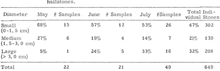
2. Size - The mean size (diameter) of the 610 hailstones analyzed was 1. 83 centimeters.

The hailstones were separated into three different categories; small

hailstones, medium hailstones and large hailstones. The frequency of

occur-rence of hailstones of each category is shown in Table 1. Table 1 shows that

Table 1. Frequency of occurrence of small, medium, and large

hailstones.

Diameter May #Samples . June

#

Samples July iSamples Total Indi

-victual Stones Small · 68% 15 57% 12 53% 26 4 7% 302 (0-1. 5 cm) Medium 27% 6 19% 4 14% 7 21% 139 (1.5-3.0 cm) Large 5% 1 24% 5 33% 16 32% 208 (> 3. 0 cm) Total 22 21 49 649

68 percent of the individual stones were small and medium size.

H

o

wever

.,

~e:.S,~ data are biased towards the occurrence of large hailstones, because the coopera

-tors tend to collect the largest hailstones for a hail sample. It would be more

correct to say that small and medium sized hailstones made up about 90 percent

of the hailstones that fell in 196 2. ·

3. Ice crystal ratio - The frequency of small (r < 1) and large (r > 1) ice crystal ratios was calculated. The results are shown in Table 2. As may

be seen from Table 2, 46 percent of the hailstones had large ice crystal ratios,

(hailstones containing a greater volume of small ice crystals) and 54 percent had

small ice crystal ratios (hailstones containing greater volume of large ice

Table 2. Frequency of occurrence of small and large ice crystal

ratios.

Total May June July

# Samples # Samples # Samples # Samples

r < 1 54% 341 63% 14 29% 6 61% 30 (Greater volume of large cry -stals) r > 1 46% 293 37% 8 71 % 15 39% 19 (Greater volume of small crystals) Total 634 22 21 49

4. Growth rings - The total volume of ice from the 610 hailstones that

were analyzed was 13,382 cm 3. This volume was calculated by assuming each

hailstone was a spheroid having a diameter equal to the greatest length. The

corresponding volume of small ice crystals was 6,415 cm 3, and the volume of

the large ice crystals was 6, 967 cm3• This indicates that during the summer

there was a greater volume of hail formed from large ice crystals than from

small ice crystals.

Analysis was made of 257 hailstones to determine the number of wet and

dry growth rings. The average number for both wet and dry grovvth rings was

found to be 1. 3. This indicates that the mean hailstone for 196 2 contained about

one dry growth ring and one wet growth ring. However, there were many hail -stones with 3 grmvth rings and a few that contained as many as 8 growth rings.

5. Embryo diameter - The mean embryo diameter for 257 hailstones

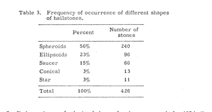
analyzed was . 08 centimeters. The range was from . 01 to . 16 centimeters. 6. Hailstone shape - Analysis of shape was made for 427 hailstones. The results are given in Table 3. Table 3 shows that the greatest number of hailstones were shaped as spheroids or ellipsoids*.

The method for categorizing hailstones and hailstone embryos were discussed

in the section on Data Analysis. It is sometimes difficult to distinguish the

difference between a spheroid and an ellipsoid, therefore, the spheroids and

ellipsoids should be considered as one shape. The other categories are very

Table 3: Frequency of occurrence of different shapes of hailstones. Percent Number of stones Spheroids 56% 240 Ellipsoids 23% 96 Saucer 15% 66 Conical 3% 13 Star 3% 11 Total 100% 426

7. Embryo shape - Analysis of shape of embryo was made for 407 hail-stones. The results are shown in Table 4. The "undetermined" shapes are the hailstones which had no distinguishable embryo. Table 4 shows that the majority of the hailstones embryos were shaped as spheroids or ellipsoids.

Table 4. Frequency of occurrence of embryo shape for 407 hailstones.

Percent Number of stones Spheroids 68% 277 Ellipsoids 5% 19 Conical 5% 19 Undetermined 22% 92 Total 100 407

8. Type of embryo - The type of embryo (wet or dry) was analyzed from 326 hailstones. It was determined that the dry embryos appeared 54 per-cent of the time and the wet embryos 46 percent of the time.

9. Summary - From the foregoing calculations, the mean hailstone structure for the summer of 196 2 can be summarized as follows:

Mean Hailstone Structure Size ( diameter)

₌

1. 83 cm

Shape

₌

Spheroid or Ellipsoid

Density

₌

. 888

Ice crystal ratio

₌

1 or less

Number of dry growth rings = 1 Number of wet growth rings = 1

Diameter of embryo = . 08 cm

Shape of embryo

₌

Spheroid or. Ellipsoid

B. Hailstone parameter means and variability by months

The hailstone data were categorized by months. The mean and standard

deviation of each parameter were computed by months, and comparisons were

made between months. The results are shown in Table 5.

Table 5. Mean hailstone parameters (x), standard deviations (s) and number

of samples (N)

May June July Season

Para-meter -_{X s N}

-

_{X s N}

-

_{X s N}

-

_{X s N} Den- . 886 . 015 145 .883 . 014 107 .895 .012 358 . 888 . 014 257 sity Ice 38 24 145 4.8 8.8 107 4.6 30.6 358 crystal ratio, r Stone 1. 4 . 6 145 1. 9 1. 8 107 2. 2 1. 7 358 1. 8 3 1. 63 257 dia., cm Em- . 06 . 03 75 . 06 . 05 67 . 08 . 05 310 bryo dia. (dry) cm Em- . 08 . 03 75 . 10 . 05 67 . 08 . 05 310 bryo dia. { wet) cm

1. Density - From Table 5 it may be seen that the hailstones analyzed

for the month of June had the lowest density and those analyzed for the month

of July had the highest density. The difference between May and June (0. 003) is not considered significant, since it is of the same order as the accuracy of

measurement.

2. Ice crystal ratio - If the density measurements are correct, one

would expect that the ice crystal ratio of the hailstones for May and June would

be larger than the ice crystal ratio of hailstones in July. The greater the amount

of small ice crystals in a hailstone the less dense the hailstone becomes because

the small ice crystals are surrounded by many more· air bubbles than are the

large ice crystals. From Table 5 it may be seen that May and June do have

larger ice crystal ratios than July, which indicates that the hailstones in May

and June had proportionally more small ice crystals than in July.

3. Size - Table 5 shows that the mean hailstone diameter was smallest

in May ( 1. 4 cm) and largest in July ( 2. 2 cm). These data are consistent with the

idea of thunderstorms in late June and early July having higher cloud tops and

being more vigorous than the thunderstorms in May and early June. It seems

reasonable to believe that the thunderstorms with high cloud tops and large

verti-cal velocities produce the larger hailstones, since the hailstone will have

far-ther to travel in the cloud, and must also obtain a greater mass to overcome the

strong vertical current before falling to the ground.

Hailstone diameters were divided into three different size categories

for May, June and July. The frequency of occurrence was then determined for

each category for each month. (See Table 1.) From Table 1 it may be seen that

May had the greatest frequency of small hail, and the lowest frequency for large

hail. June had less small hail than May, and more large hail than May, and

more large hail than May. July had the least amount of small hail and the

greatest amount of large hail. These data also lends support to the idea that

late June and early July are the months with the most vigorous thunderstorms.

4. Embryo diameter - From Table 5 it may be seen that the diameter

of the wet and dry embryos are uniformly distributed for the three months.

C. Hailstone parameter means and variability by geographic areas

The hail network in northeastern Colorado was divided into four quadrants

(See Figure 4) The mean value and standard deviation of each hailstone parame-ter were then calculated for each quadrant. The results are given in Table 6.

Table 6. Mean hailstone parameters (x), standard deviations (s), and number of samples (N) by quadrants from Sterling, Colorado Quadrant I Quaarant II Quadrant III Quadrant IV

Para- (NE) (NW) (SW) (SE)

meter -N

-

N

-

-X s X s X s N X s N Dia., cm 2. 6 1. 6 135 1. 8 1.4 230 1. 2 1. 6 140 2. 3 2.0 165 Density .893 .013135 . 891 . 014 2-30 . 889 . 014 140 . 892 . 007 165 Wet em- . 03 110 . 03 150 . 04 100 . 03 100 bryo dia. cm Dry em- .03 110 . 04 150 . 04 100 . 04 100 bryo dia. cm

From Table 6 it may be seen that the eastern quadrants have the larger hailstones. This difference could be attributed to the fact that the thunderstorms

form in the lee of the Rocky Mountains and move east. The maximum cloud tops

are not attained until the thunderstorms are 50 to 60 miles east of the Rocky

Mountains. This vvould put the thunderstorms just east of Sterling, Colorado at

the time maximum cloud tops are attained, he nee, the larger hailstones should

fall in eastern Colorado.

The densities of hailstones vary little between quadrants . .

There is no significant difference in the diameters of the embryos for

the four different quadrants.

V. SIMPLE CORRELATIONS

A. Total analyzed hailstones

Using the 1620 IBM computer and the Esso Stepwise Multiple Linear

Regression Analysis Program, simple correlations behveen hailstone size

(diameter), density, ice crystal ratio, number of dry growth r:i,ngs, number of

wet growth rings, and diameter of embryo were made.,:, These correlations

Table 7. Simple correlation coefficients for all ( 25 7) hailstones. Diame -ter Ratio No. of No. of dry growth · · rings Diameter of embryo Density Diameter 1. 00 wet growth r'ings · 0. 02627- 0. 14543* ,:, 0. 05585- 0.04000 )f.';f. Ratio 1. 00

o.

12281- 0.04515- 0. 05239-

o.

1 6427-No. of wet growth rings No. of dry growth rings Diameter of embryo Density 1,00 0, 28380':o:, 1. 00

,:, indicates significance at the 5 percent level

>i":'indicates significance at the 1 percent level

0.09500- 0.07301

*"~

0.17875- 0. 01121

1. 00 0.0

7974-,t. 00

Looking at Table 7, we see that only two parameters (number of wet

growth rings and the number of dry growth rings) have a significant correlation with hailstone diameter. There is significant negative correlation between ice crystal ratio rings and density. This result indicates that as the ice crystal ratio increases, the density of a hailstone decreases. This result is reasonable, since a large ice crystal ratio should mean that there are more small ice cry

-stals than large ice crystals, and therefore, a lower density.

There is a significant positive correlation between the number of wet

growth rings and the number of dry growth rings.

There is a significant negative correlation between the number of dry growth rings and the diameter of the embryo.

B. Hailstone parameter correlations by months

Correlations of each hailstone parameter with other parameters were

made for each month separately. The number of observations for each month was as follows: May = 27, June = 50, July = 180. The results are given in Tables 8, 9 and 10.

Table 8. Simple correlation coefficients for May (27) hailstones. Diameter Ratio No. of wet growth rings No. of dry growth rings Diameter of embryo Density

Diame- Ratio No. of

ter wet growth

rings 1. 00 0. 43275'~

o.

20018 1. 00

o.

21713-1. 00 No. of dry growth rings 0,11517 0. 07742 0. 34069,:, 1. 00

*indicates significance at the 5 percent level

Diameter Density

of embryo 0.17529

o.

186 42-0.2273-

o.

27348 0.31769-

o.

29209

o.

37300- 0.04677 1. 00 0.21989 1. 00

Table 9. Simple correlation coefficients for June (50) hailstones.

Diame- Ratio ter No. of wet growth rings Diameter 1. 00 0.17011 0.17705 Ratio No. of wet growth rings No. of dry growth rings Diameter of embryo Density 1. 00 0.203 22-1. 00 No. of dry growth rings

o.

34 7 35,:, 0.21157 0,08115 1. 00

*

indicates significance at the 5 percent level ,:o:,indicates significance at the 1 percent level

Diameter of embryo

o.

03769

o.

10 346 -0. 16717-~~*

o.

45248-1. 00 Density

o.

54907,:":, 0.1610 4- 0,09297-

0.03266-o.

30715->:' 1. 00

Table 10. Simple correlation coefficients for July (180) hailstones. Diame -ter Diameter Ratio No. of wet growth rings No. of dry growth rings Diameter of embryo Density 1. 00 Ratio No. of wet growth rings 0. 0 6 6 34 - 0. 1 7 14 5 ,:, 1. 00

o.

1130 6-1. 00 No. of dry growth rings 0.068

06-o.

368 36 ,:o:, 1. 00

,:, indicates significance at the 5 percent level

:(o:,indicates significance at the 1 percent level

Diameter of embryo

o.

10854 -0.0562 8-0.05400 -0. 093 43-1. 00 Density 0. 246 30,:o:, ~.:>.';

o.

1 9626-0.05736 0.06774 0.04137 1. 00

Looking at Tables 8, 9, and 10, it may be seen that eleven have

signifi-cant correlations. These correlations are listed below: May

Diameter vs ice crystal ratio

Number of wet growth rings vs number of dry growth rings

June

Diameter vs density

Diameter vs number of dry growth rings

Number of dry grovvth rings vs diameter of the embryo {negative)

Diameter of the embryo vs density {negative) July

Diameter vs number of wet growth rings

Diameter vs number of dry growth rings

Diameter vs density

Ice crystal ratio vs density (negative)

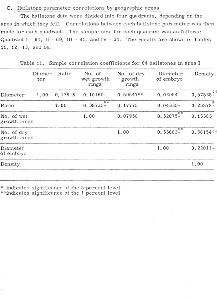
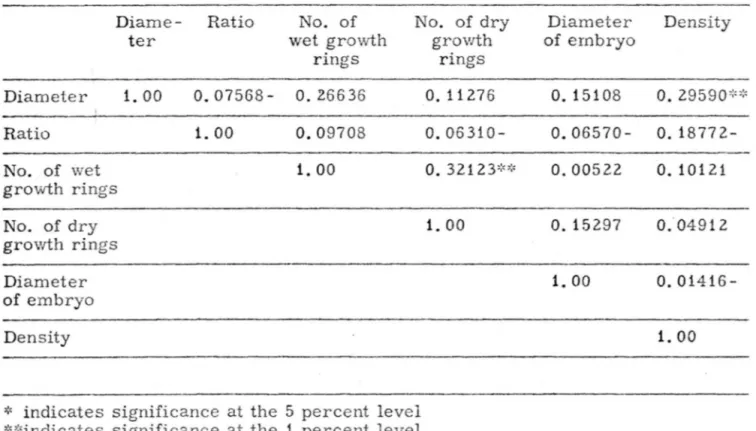
C. Hailstone parameter correlations by geographic areas

The hailstone data were divided into four quadrants, depending on the

area in which they fell. Correlations between each hailstone parameter was then

made for each quadrant. The sample size for each quadrant was as follows:

Quadrant I= 64, II= 69, III= 81, and IV= 34. The results are shown in Tables 11, 12, 13, and 14.

Table 11. Simple correlation coefficients for 64 hailstones in area I Diame- Ratio

ter Diameter Ratio No. of wet gro·wth rings No. of dry growth rings Diameter of embryo Density 1.00 0.13818 1. 00 No. of No. of dry

wet growth growth

rings rings 0. 10160-

o.

5954 7t_:,;, :::~ :i:: 0.38725-

o.

17775 1. 00 0.07936 1. 00

*

indicates significance at the 5 percent level **indicates significance at the 1 percent level

Diameter Density of embryo ,:,,:, 0.02964

0.57838-*

0.04339- 0.25 878-~::,;c 0. 32075- 0. 13363 )!c>!(

o.

33062- 0. 36 154 ,::,:, 1. 00 0. 22011-1. 00

Table 12. Simple correlation coefficients for 69 hailstones in area II

Diame- Ratio No. of No. of dry

ter wet growth growth

rings rings Diameter 1. 00 0.06464

o.

17322 0.03017 Ratio 1. 00 0.13890- 0.06 679-No. of wet 1.00 0. 23541* growth rings No. of dry 1. 00 growth rings Diameter of embryo Density

,:, indicates significance at the 5 percent level

*':'indicates significance at the 1 percent level

Diameter Density of embryo 0.04265- 0. 16965

*

0.07253- 0.264 87-0. 12922-

o.

15459 0. 20748 0. 31518':,,:, 1. 00 0.22341 -1. 00

Table 13. Simple correlation coefficients for 81 hailstones in area III

Diame- Ratio No. of No. of dry

ter wet growth rings Diameter 1. 00 0.07568- 0.26636 Ratio 1. 00 0.09708 No. of wet 1. 00 growth rings No. of dry growth rings Diameter of embryo Density

,:, indicates significance at the 5 percent level

,:o:,indicates significance at the 1 percent level

growth rings

o.

11276 0.063 10-0. 32123,:o:, 1. 00 Diameter Density of embryo

o.

15108

o.

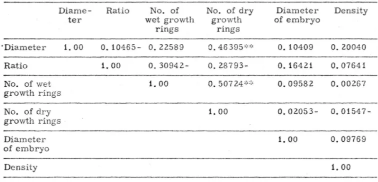
29590':":' 0.06570- 0. 18772-0.00522 o. 10121 o. 15297 o.·04912 1. 00 0.01 416-1. 00

Table 14. Simple correlation coefficients for 34 hailstones in area IV 'Diameter Ratio Diame-ter 1. 00 No. of wet growth rings Ratio No. of wet growth rings 0. 10465-

o

.

22589 1. 00 0. 30942-1. 00

No. of dry Diameter Density growth of embryo rings 0. 46395,:,,:,

_o

_.

_{10409 0. 20040} 0. 28793- 0. 16421 0.07641 0. 507 24,:<>:, 0. 09582 0.00267 No. of dry growth rings 1. 00

o

.

02053-

o

.

01547 -Diameter of embryo Density

*

indicates significance at the 5 percent level ,;"~indicates significance at the 1 percent level

1. 00 0.09769

1. 00

From Tables 11, 12, 13 and 14, it may be seen that the significant cor-relations were as follows:

Quadrant I

Diameter vs number of dry growth rings

Diameter vs density (negative)

Ratio vs number of wet gro\vth rings (negative) Wet growth rings vs diameter of embryo

Dry growth rings vs density

Dry growth rings vs diameter of embryo (negative) Quadrant II

Ratio vs density (negative)

Number of wet growth rings vs number of dry growth rings

Number of dry growth rings vs density.

Quadrant III

Diameter vs density

Number of wet growth rings vs number of dry growth rings. Quadrant IV

Diameter vs number of dry growth rings.

VI. PREDICTION OF DENSITY FROM OTHER HAILSTONE PARAMETERS

A. Prediction equations by months

Using the Esso Stepwise Regression Program on the 1620 Computer, the hailstone density was computed as a function of the other hailstone parameters.

Using the density as the dependent variable, and the other five variables as independent variables, their program computes the variables, single or as a group, would be the best for predicting the density of a hailstone. This was done by computing the standard error of Y for each group of independent vari-ables, and choosing the single or group of variab:es with the lowest standard error of Y . where Y = K+C 1 X1 +C2 X3

+c

3

x

4

+c

5

x

5 Y = Density

x

₁ = Hailstone diameter

x

₂ = Ice crystal ratio

x

₃ = Number of dry growth rings

x

₄ = Number of wet growth rings

x

₅ = Diameter of embryo.

The results of these computations are as follows: May

y

= • 889 - . 007

x

1 + . 001 X4 June y = • 905 - • 004 x 1 + . 008 X5 July Y = .89+.002 X 1

B. Prediction equations by quadrants

Using the same procedure as described above for months, prediction equations for density were computed for each ge graphic area (See Figure 4). The results were as follows:

Quadrant I

Quadrant II y = • 889 + . 003 x i - . 00005 x 2 Quadrant III. y = • 889 + • 002s x i - . oooos x 2 Quadrant IV y = • 898 - . 0007 x 1

VII. ANALYSIS OF VARIANCE

A. F Tests

-An analysis of variance was performed to determine if these were signi

-ficant differences tin hailstone diameter between months. The results indicated

highly significant differences (at the i percent level):

A similar computation indicated highly significant differences in

hail-stone density between months.

An analysis of variance was performed to determine whether significant

differences existed between geographic areas for hailstone parameters of d

ia-meter and density. The results indicated highly significant differences for both

parameters.

B. Students

"t"

tests

Students

"t

II

tests were then applied to determine which of the above

fac-tors were significantly different when considered on an individual basis.

The results of this test applied to the parameter of hailstone diameter

I

indicated that the only significant difference was between May vs June and July.

The results of the test applied to the hailstone density also indicated a

significant difference between May vs June and July. The student "t II

test was applied to hailstone diameter for the four

geo-graphic areas shown in Figure 4. The results indicate significant differences

in hailstone diameter between area I vs II, area II vs IV, and area III vs IV.

A similar computation for hailstone densi:y indicates significant

dif-ferences in mean hailstone densities between area I vs

III.

and area I vs IV.

VIII. CORRELATION BETWEEN HAILSTONE ffi RAMETERS

AND THUNDERSTORM PARAMETERS

Hailstone parameters of diameter and der:sity were plotted against

cor-responding thunderstorm parameters of radar tops, Z , and "tilt of

echo. The results are given in Figures 5-10.

From Figure 5 it may be noted that there are no large hailstone diameters

(greater than 3. 5 centimeters) having radar echo tops below 45, 000 feet. This

scatter diagram indicates that high cloud tops do not mean that only large

hail-. stones will form, but that it is necessary to have high cloud tops to have large

hailstones.

Simple correlation coefficients were computed between each of the

parameters listed above. The results are shown in Table 15.

Table 15. Simple correlation coefficients between hailstone

Radar Tops

z

Tilt

max

r d. f. r d. f. r d. f.

Diameter • 06 22 • 41 i6 . 13 13

Density . 17 22 . 21 16 .47 13

None of the correlations were significant at the 5 percent level.

IX. SUMMARY AND CONCLUSIONS

During the summer of 196 2 hail samples were collected. Eight hai

l-stone parameters were determined. The mean and variance of each hailstone

parameter was determined by various groupings. The simple correlation coe

f-ficients between the hailstone parameters were determined. An analysis of

variance using the test was applied to determine significant differences of

hail-stone parameters between months and geographic areas.

The average hailstone for the summer of 196 2 had the following mean

parameters:

Size (diameter)

Shape hailstone

Density

Ice crystal ratio

Number of dry growth

rings = 1. 8 3 centimeters = Spheroid or Ellipsoid = • 888 = 1 = 1

Number of wet growth rings Diameter of embryo Shape of embryo = 1 = • 08 centimeters = Spheroid or E lipsoid

On a seasonal basis, May had the lowest mean hailstone diameter and

July had the largest. June had the least dense hailstones and July had the most

dense hailstones. The other hailstone parameters; ice crystal ratio, embryo

diameter, and the number of wet and dry growth rings, did not vary much.

The fact that the mean hailstone diameter was larger in June and July can be attributed to the fact that thunderstorms in late June and early July have, on the average, higher cloud tops and are more vigorous than the thunderstorms

in May or early June. This would mean that a hailstone would have further to travel in a cloud and would have to develop a greater mass to overcome the

stronger vertical velocities.

On a geographic basis the hailstones east of Sterling, Colorado, have a

larger mean hailstone diameter than the hailstones west of Sterling. This is

probably due to the fact that the majority of the thunderstorms form in the lee

of the Rocky Mountains and move east. The max cloud tops are not reached until

they approach the Sterling area. These thunderstorms would then be producing

their largest hailstones, which would be falling in eastern Colorado. The other

hailstone parameters did not vary significantly.

The standard deviation of the total analyzed hailstones was large. On a

seasonal basis May had the lowest standard deviation for hailstone diameters

while June and July had large standard deviations. This would indicate that in

May the hailstones were mostly S!Tlall, while in June and July the hailstones

con-sisted of both small and large diameters. For density, May had the largest

stan-dard deviation, and June and July the lowest.

The Esso Stepwise Multiple Linear Regression Analysis was applied to

various groups of data to give equations of the following form for predicting

hail-stone density, the following formula:

Density= K+C

1 X1 +C2 X2 +c3

x

3 +C4 X4 +C5 X5

An analysis of variance using the F test and students' t tests showed

that there were significant seasonal and geographical differences in hailstone

The simple correlation coefficients between the physical properties of a hailstone and the radar properties of a thunderstorm failed to yield any signi-ficant results. This was probably due to small sample sizes and the methods . used for determining from which thunderstorm a certain hail sample fell.

X. REFERENCES

1. Eaton, Larry. Hailstone Structure Studies, 1960-1961. Unpublished report, Civil Engineering Section, Colorado State University, 196 2.

2. Schleusener, R. A., and J. D. Marwitz. Characterisaics of Hailstones on the High Plains as Deduced from 3 cm Radar Observations. Proc. Ninth Weather Radar Conference, 196 2.

1

2

"

I I I I I I I I I I - - - -- - 1- - -- -- -- -- -- -- -- -- -- -- -- -- -- --- - 1- - - - -1 I I - - -- - -- - - -

- -

,

--

- -

-I - - - -1 -1 I I I I I I I I I I

_ . _ _ _ - - . + - t - + - - t - -

2 P

olar

i

zed

l

ens

~---,,<-t

--+-+---

1

P

o

I

a r

i

zed

I

ns

- - - - -

G

l

ass p

l

ate

)

-

-

-

--

-

~

-/ / / / / / / / / / / / / / / / / / / ___,__ LL/ _ _ _ _ _ _ _ _ _ _ _ _ , ¥

F

i

g

. I

Ph

ot

o ox

_/zScal

Con ains CCI 4 n paint

t r.

~

- -

;..._

2

50 m

l Fl

as

.

-

On

e

:J

a

ll

o

n

can.

- - ---4-- Contains alcohol and

v1ater

.

Sida

Vi

e

v

Y2

Seal

>,

+->

₀ .... . 006 O' -~ ~

~

Ill 0 .... 004 0 .... .... w .002 - ---·---·-- ---- -

__

..._

____

_,_____

__

_

__, '

-

-

-

- - -

-

-

1

- - -

- - -

-

- -

-

- - - - -

-

32° F

l

35 30 25 20 15 TEMPERATURE F 0

IT

_I

.

.

Osidney

Q

Chappel

0

.

_·o·

Jule:ibur~

•

.

•

.

Sed~wk:lc •

..

. .

.

.

.

.

.

_• • •

.

_.

.

,-t--. • \.LI • Sterling

..

_•

0

•• Holyo\e

.

..

• _•

.

•

.

.

:

...

.

.

0

0

I[

.

0

Fig. 4 Map of four geographic areas. Dots show locations

(2) 0 50 - A '-'

I

1v 0 0 0

I

I

I I 0 I

I

I _' 45 I-LL Y'. I _! I ,.... ,.... - ...:, ' - '

I

I '-' I I

I

I I _! I 0 I :

I

I

I

I

I I I _I Ul 0. 0 I-.... 0 40 "O 0 0:: I I 0 I

I

I I

i

I

I

I

I I I I _!

i

I I 0 I I i I I

I

0 I I

I

I I ! I I ' I 35

I

_I ' ' ! '

I

I I

I

I

I

_'

I

I

l

I

I

I 0 0 0 2 3 4 5 6 Hailstone diameter (cm)

~ 8) E N a, 0 0 lj() 20

•

I

..

~-

. _• r I t - - - -• - - · - - _ _ _ .._ __ ·- - - < - - - - -- - - 1 - -- - l

--:--- -

--- --

~-

-- ---- - -

--·---+---1--

---:l

I - - - - -- > - - - - . _ _ _ - - -~ - - - -- - I - - - - ----+- - - + - - - l

!

I

--- ---1

--- -

-7

1----

---.---l---

·

-- - --

- - - -+; _ _ _ _ _ I _ _

I

=1

i

---

---

·

----·----J

____ -- - -

- - - 4 - - - ---'

I

____

j

2 3 4 5 6

Hailstone diameter(cm)

·

-50 r, ,.., 0 40 0 _r. ~ 30

-

o

d

z

)

10 O(Z) 9 0 r. 2 3 4 5 Hailstone diameter (cm)

I.I) a. 0 I-... 0 -0 0 n:: 0 0 0 50r----r-~~---➔ ---4---8B--t-<°r-~F'J---i 0 0

I

·-

0 0 45 I

-

-i

-

-I 0 40 r - -- -,- -- ~-- - - -~;--- fl8r - - + - - - - ~

I

0 0 I

I

I

I

35 l--,--- - - + -- - - + - - --t-- - -- r - - ---1 0 0 0 ~ - -- ·- -- _J _ __ _ -- - - L - - ---' 0.87() 0.880 0.89'.) 0.900

Hailstone density

X. 0 E N C7l 0 0 60 40 20 Fig.

9

0 ₀

~

u cP 0 (, 0 ~

-

~ 0.8tD 0.880 0.890 0.900 0.910 Hailstone density

o

_{..__.,,} 40 0 u ~ L (l.) > 30 E C

_....

-.... 20 f-10 0 0

/ '

V

]/v 0

l

/o

0 0

/

(

Vero

(

0 0

V

~ -- 0 0870 0.880 0.8 0.900 0.910 Hails tone density

Fig 10 Scatter diagram of hoi'1stone density vs. ti It.