Trading Volume : The behavior in information asymmetries

I

H

HÖGSKOLAN I JÖNKÖPING

Trading volume

The behavior in information asymmetries

Master’s thesis within finance

Authors: Johansson Henrik,

Wilandh, Niklas

Tutor: Ekon. Lic. Magnus Hult Examinator: Gunnar Wramsby

Master’s Thesis in Finance

Title: Trading Volume

Authors: Henrik Johansson

Niklas Wilandh

Tutor: Magnus Hult

Date: [2005-06-06]

Subject terms: Finance, stock market, trading volume, information asymmetry

Abstract

Background According to theory, trading volume decreases in information asymmetries,

i.e. when there are differences in information. This is due to the fact that uninformed investors delay their trades when they are facing adverse selec-tion. When the asymmetry is resolved there should be a corresponding in-crease in trading volume. Around earnings announcements (scheduled an-nouncements) this asymmetry is greater than normal, hence one can expect a decrease in trading volume. Around unexpected announcements such as acquisition announcement (unscheduled announcements) a total increase is instead expected because of an increase in trading by informed investors. All these effects are likely to be greater for smaller stocks.

Purpose The purpose of this thesis is to investigate the trading volume before- and after scheduled announcements and the trading volume before unscheduled announcements in order to investigate how informed- and uninformed in-vestors behave in information asymmetries on Stockholmsbörsen.

Method The method is quantitative with secondary data from the Stockholm Stock exchange from 1998-2004. The method is the same as Chae (2005) uses with paired-samples t-tests. It tests whether the change in trading volume is different from a benchmark consisting of an average of the trading volume 30 days before the announcement.

Conclusion We found a statistically significant decrease in trading volume in 6 of 10

days before a scheduled announcement and an increase also on 7 of 10 days after the announcement. For unscheduled announcements we found an in-crease before it was released but were not able to prove it statistically. We conclude that uninformed investors behave strategically before scheduled announcements in order to avoid adverse selection. We could not conclude that the effects are greater for smaller stocks.

Innehåll

1

Introduction... 1

1.1 Background ... 1

1.2 Research problems ... 1

1.2.1 Research problem 1: The trading volume should decrease before a scheduled announcement. ... 2

1.2.2 Research problem 2: There should be a corresponding increase in trading volume after the scheduled announcement is released. ... 2

1.2.3 Research problem 3: The trading volume should increase before an unscheduled announcement... 3

1.2.4 Research problem 4: All the assumed effects should be greater on smaller firms. ... 3

1.3 Purpose... 4 1.4 Definitions ... 4 1.5 Disposition... 5

2

Method... 6

2.5 Summary of technical method... 7

2.6 Data Collection... 8

2.6.1 Stockholmsbörsen ... 8

2.6.2 Waymaker ... 9

2.7 Analyzing data... 9

2.7.1 Preliminary study ... 9

2.7.2 Calculating trading volume ... 9

2.7.3 Analyzing trading volume... 10

2.7.4 Robustness tests ... 10

2.8 Reliability and validity ... 10

2.8.1 Validity ... 10

2.8.2 Reliability ... 11

3

Theoretical framework ... 12

3.1 The importance of trading volume... 12

3.2 Noise ... 13

3.3 Trading volume in information asymmetries... 14

3.3.1 Trading volume prior to scheduled announcements ... 14

3.3.2 Trading volume after scheduled announcements ... 15

3.3.3 Trading volume around unscheduled announcements... 15

3.4 Critique of the theoretical framework... 16

4

Previous Studies ... 17

4.1 Trading Volume, Information Asymmetry, and Timing Information... 17

5

Empirical findings ... 19

5.1 Preliminary study... 19

5.2 Main study... 19

5.2.1 Scheduled announcements ... 20

5.2.2 Unscheduled announcements ... 21

5.3 Comparison A-listan and O-listan... 22

5.3.1 Scheduled Announcement... 22 5.3.2 Unscheduled Announcements... 23 5.4 Robustness check ... 24 5.4.1 Scheduled announcements ... 25 5.4.2 Unscheduled Announcements... 26

6

Analysis... 27

6.2 The result’s relation to theory ... 28

7

Conclusion and Final Discussion ... 30

7.1 Conclusion ... 30

7.2 Final discussion... 31

7.3 Suggestions for further studies... 32

Figurer

Figure 1.6, Disposition of the thesis. ... 5

Figure 2.2, Simplified description of noise... 13

Figure 5.1, Histogram for log turnover (left) and non log turnover (right) ... 19

Figure 5.2.1, Turnover around scheduled announcements... 21

Figure 5.3. Comparison A-listan/O-listan, Scheduled announcements. ... 23

Tabeller

Table 2.1. A synthesis of important result on price-volume correlations (Source: Karpoff, 1987) ... 12

Table 4.1. Daily Abnormal Turnover around Different Events. T-value in parenthesis (Source: Chae, 2005)... 17

Table 5.1. Descriptive statistics from preliminary study... 19

Table 5.2. Daily Abnormal Turnover around Different Announcements ... 20

Figure 5.2.2, Turnover around scheduled announcements... 22

Table 5.2. Daily Abnormal Turnover around scheduled announcements for A- and O-listan ... 23

Table 5.2. Daily Abnormal Turnover around scheduled announcements for A- and O-listan ... 24

Table 5.3. Robustness test: Daily Abnormal Turnover around Different Announcements ... 25

Figure 6.1, Comparison of studies around scheduled announcements... 27

Figure 6.2, Comparison of studies around unscheduled announcements.... 28

Appendix

1 Introduction

In this chapter we will present the background and the research problems of the studied subject. Then the hypotheses are stated and explained along with the purpose of the thesis. Further, we will explain some of the definitions used in the thesis and finally show the disposition.

1.1 Background

Trading volume is what drives the financial markets. It makes it possible for investors to become stockholders and for companies to raise capital. The trading volume is not con-stant, it varies considerably over time. We assume that investors select when to trade on the basis of information. The volume can be seen as an indicator for information asymmetries among investors. According to Karpoff (1987) many studies show that the price of a secu-rity gives a signal on how the market evaluates new information, while the volume hints about different opinions among investors on how to interpret the new information. On a financial market investors trade among each other because they have different knowledge and beliefs about a given security, otherwise there would not be any trading. Therefore, as Wang (1994) states, the behavior of the trading volume is closely linked to the underlying heterogeneity among investors.

The investors on financial markets can roughly be categorized in two groups, informed in-vestors and uninformed inin-vestors. The informed inin-vestors trade on the basis that they have information about a security that is not publicly known, i.e. private information. These in-vestors trade in order to reap future payoffs. The uninformed inin-vestors, on the other hand, trade for other reasons. One is liquidity, included in this category are large financial institu-tions that trade merely for liquidity needs of their clients or to balance their portfolios (Admati and Pfleiderer, 1988). This fact creates an adverse selection problem, where the uninformed investors have a disadvantage in terms of information. Around corporate an-nouncements when a great deal of information is released, the information asymmetries be-tween informed and uninformed investors are believed to be the greatest. Thus, it is rea-sonable to believe that around these announcements, the uninformed investors know they are facing adverse selection and reduce their trading.

There exist several theoretical models on the behavior of trading volume prior to corporate announcements. E.g. Foster and Wiswanathan (1990) developed a model where the trading volume decreases on Mondays because that is the day of the week when informed traders have the biggest advantage in terms of information, and therefore the day when informa-tion asymmetries are the greatest. Or in Admati and Pfleiderer (1988) where uninformed investors concentrate their trading strategically in order to avoid adverse selection problems around information releasing events. Milgrom and Stokey (1982), Black (1986) and Wang (1994) also theorize about this and have developed models where uninformed investors will decrease their trading if they risk trading against informed investors. Yet, one theoreti-cal model contradicts the implications of the mentioned models. In Kyle (1988) the trading volume increases before corporate announcements because the informed investors are ea-ger to exploit their informational advantage.

1.2 Research

problems

Still, this subject is, empirically, almost unexplored. As we know of, only Chae (2005) has attempted to empirically test the trading volume prior to and after corporate

announce-ments and relate it to information asymmetries. His results were that the trading volume decreases just prior to scheduled corporate announcements (earnings announcements). Be-fore unscheduled announcements (e.g. Acquisitions, Moody’s ratings), the volume in-creases. He also found that the trading volume before scheduled announcements is nega-tively correlated with proxies for information asymmetry.

This thesis is dedicated to further test the empirical implications of trading volume in in-formation asymmetries. This time a smaller stock exchange will be tested, i.e. the Stock-holm Stock Exchange (StockStock-holmsbörsen) in order to see if the results of Chae hold in a different setting. We attempt to study how the trading volume behaves prior to and after unscheduled corporate announcements. This will lead to a further understanding for how different kinds of investors behave in situations when they face divergences in terms of in-formation. Hence our research problems:

1.2.1 Research problem 1: The trading volume should decrease be-fore a scheduled announcement.

Taking into account the implications of the models of Wang (1994) and Foster and Wiswanathan (1987) trading volume should decrease prior to a scheduled announcement. Since the timing of the announcement is known to the public, the uninformed investors will know that they are facing adverse selection and decrease their trading. In an extreme case, with only one informed and one uninformed investor, the informed investor wants to exploit his advantage and trade before the information is publicly known (Chae, 2005). This is almost impossible, however, because the uninformed investor knows that she has a clear disadvantage and wants to trade only if there is an urgent liquidity need. This leads to a situation where no trading is present.

Deciding the pattern of trading volume prior to scheduled corporate announcements when there is a great deal of information asymmetry involved is an addition to the current re-search about trading volume and how different investors act in information asymmetries on financial markets. This may suggest that differences in beliefs are the main determinant of trading volume. It could guide investors about taking decisions on whether to trade or not before corporate announcements in order to obtain a desired influence on the price of the stock. Studies have shown that there is a clear price/volume relationship on financial market so a sudden increase in trading volume is very likely to have an effect on the stock price. As Admati and Pfleiderer (1994) put it; investors prefer to trade when the market is “thick”, i.e. when their actions have little effect on prices.

1.2.2 Research problem 2: There should be a corresponding increase in trading volume after the scheduled announcement is re-leased.

According to the theory of George et. al. (1994) when the announcement is released the in-formation asymmetry is resolved. This makes the transaction costs decrease significantly because the market maker narrows the bid-ask spread. This induces uninformed investors to trade and the effect would be an increase in total trading volume.

This problem is part of our aim to pinpoint the behavior of uninformed and informed in-vestors. For the decrease before scheduled announcements to make sense there must be an increase after the announcements is released and there is symmetric knowledge.

1.2.3 Research problem 3: The trading volume should increase before an unscheduled announcement.

This problem is derived from the fact that the timing of an unscheduled announcement is not publicly known and therefore, the uninformed investors have no possibility to plan their trades strategically and will trade just as usual. The informed investors, on the other hand, have an advantage in terms of information and want to exploit this before the an-nouncement is released. This will lead to an increase in informed trading and thus an in-crease in total trading volume (Chae, 2005).

This problem is partly set up to confirm the first two problems. If it is true that unin-formed investors anticipate that they have a disadvantage in terms of information before announcements for which the timing is publicly known and decrease their trading accord-ingly, then there should be now way for them to anticipate their disadvantage before un-scheduled announcements. That implies that the decrease in trading volume before sched-uled announcements must originate from uninformed investors. The increase in trading volume before unscheduled announcements, on the other hand, should come from in-formed investors. This could be helpful in investment strategies for uninin-formed investors. If there has been an observed significant increase in trading volume for a few days in a row it is likely that the increase is due to trading on private information and that the company in question is about to make an important announcement.

1.2.4 Research problem 4: All the assumed effects should be greater on smaller firms.

One main theoretical foundation of this thesis is that information asymmetries are driving the trading volume down before scheduled announcements. This leads to a question of what exactly is causing the information asymmetry. One factor that is likely to have an im-pact on this asymmetry is how “established” a firm is, as argued by Ritter (1984). Being es-tablished involves among other things; how old the firm is, how large it is and how well known it is. For a well established firm more information is publicly known and less people are likely to possess private information about the firm , i.e. there is less information asymmetry. As a consequence, we assume that the trading volume for less established firms is going to decrease to a greater extent compared to more established firms. The corre-sponding decrease should also be accompanied by a greater increase when the scheduled announcement is released because the greater the information asymmetry prior to the nouncement, the greater the effect of resolving the asymmetry. For unscheduled an-nouncements, we suspect a greater increase before release for less established firms. This comes from the notion that, for these firms, there are more investors with private informa-tion that they are eager to take advantage of.

We have used firm size as a measure of how established a firm is and will thus function as a proxy for information asymmetry. The usage of firm size as proxy can be justified by, among others, Atiase (1985) who empirically verifies that the amount of private pre-disclosure information dissemination is an increasing function of firm size. A random sam-ple from the larger stock index A-listan will be compared to a samsam-ple from the smaller in-dex O-listan. As demonstrated in table 1.2 the average total share value for A-listan in our sample is more than 12 times greater than average total share value for O-listan. This prob-lem could provide useful information on what firms are considerably more affected of the hypothesized behavior of trading volume.

Table 1.2 Average total share value in our random sample

Average total share value in MSEK. A-listan O-listan

58974.85 4784.91

1.3 Purpose

The purpose of this thesis is to investigate the trading volume before- and after scheduled announcements and the trading volume before unscheduled announcements in order to in-vestigate how informed- and uninformed investors behave in information asymmetries on Stockholmsbörsen.

1.4 Definitions

ƒ Scheduled announcements are in this thesis earnings announcements. Earnings reports consist of annual reports and interim reports. They report a company’s earnings on a quarterly basis. The timing of earnings announcements is known to the public. As men-tioned by Chae (2005) earnings announcements involve a release of important pricing information and are good estimations of current value.

ƒ Unscheduled announcements are any announcements, concerning a company, for which the timing is not publicly known. Here announcements regarding acquisitions of other companies are used as proxies for unscheduled announcements. These kinds of an-nouncements have well documented effects on return and trading volume as Bamber (1987) has documented.

ƒ Having private information is having more valuable information about a firm than the public has

ƒ With information asymmetries we mean that some investors have firm-specific informa-tion which is to be published in future public announcements, i.e. private informainforma-tion. Other investors do not have this information.

ƒ Adverse selection here means that some investors have an advantage in terms of infor-mation.

ƒ Investors that are uninformed in this context are investors with less knowledge than in-formed investors about the future value of a stock.

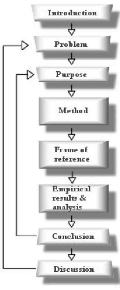
1.5 Disposition

Figure 1.6, Disposition of the thesis.

Introduction

In this chapter we give the background and motivation behind the choice of subject. The authors then discuss the problem and present the purpose.

Method

The method chapter is where the authors discuss their choice of theoretical approach and research approach. Further, we describe the way the data was collected and analyzed. Then there is a discussion around criticism against the method.

Frame of Reference

The frame of reference discusses the theory behind the subject treated. Trading volume, information asymmetry and factors behind the problem is thoroughly explained here. Other studies within the area and there finding is also dis-cussed within the theoretical framework. Finally, there is a chapter reviewing previous studies related to the subject.

Empirical Results and Analysis

Chapter 5 is where the results from the statistical tests are presented. Then the results will be analyzed and the authors will compare the result with the previous study and discuss the result against the theory used.

Conclusion and Discussion

In the last chapter we present our conclusion from the result. We will also have a final dis-cussion about our thought around the subject and finally give suggestions for further stud-ies.

2 Method

In this chapter we will discuss and motivate our choice of theoretical and research approach. We will then move on to describe how our data was collected and what method we used to analyze the data. Finally, there is a discussion around criticism towards the chosen method.

2.1 Theoretical

approach

Positivism is a development from a school of thought originating from Aristoteles, the ren-aissance and the scientific progresses of the 17th _{and 18}th _{centuries and regards absolute} knowledge as the ideal. The term “positivism” was invented by the French sociologist Au-guste Comte in the beginning of the 19th _{century. It refers to the development of positive,} i.e. absolute knowledge. Comte’s aim was to develop a scientific methodology that was valid for all scientific disciplines. According to Comte, a man only have two sources to ac-quire knowledge- what is obtainable through our 5 senses and what we can conclude by applying reasoning and logic. Positivism has its foundation in quantifying and measuring data and to this apply logical reasoning to make it possible to test scientific theories and hypotheses. According to positivism, what scientists come up with or existing theories should be testable and either accepted or rejected (Eriksson & Wiedersheim-Paul, 1999). Positivism is usually associated with objectivity, quantifying technique and generalization (Alvesson & Deetz, 2000). This is the reason why positivism views science as the highest and most valid type of knowledge. Karl Popper, a man often associated with positivism, ar-gues that the aim of the scientist is to search for true knowledge. Due to the fact that it is almost impossible to conclude that a theory is true, Popper argues that scientists should in-stead aim to reject theories. It is simpler to conclude that a theory is false than vice versa and by rejecting theories the worst ones are taken out play so that only the ones that are most true are left to be evaluated. Popper has been criticized to advocate to rigorous test-ing of new theories, so that very few of them can withstand. Instead of rejecttest-ing them many argue that they should be enhanced and improved. Thomas Kuhn had a different view on scientific philosophy than Popper. Kuhn stated that improvements in science are due to revolutionizing discoveries rather than slow evolutionary processes that Popper ad-vocates (Hult, 2003).

The purpose of our thesis is to decide the trading patterns in volume around corporate an-nouncements so a positivistic view is the given choice. Our approach is to give answer to research problems by either rejecting or accepting hypotheses.

2.2 Research

approach

According to Lekvall and Wahlbin (2001) a standpoint has to be taken whether to use a quantitative or a qualitative approach in the study. Because of the characteristics of this study our opinion is that a quantitative approach is best suited. The purpose is to make generalized conclusions from a big sample. With the quantitative data we are able to perform statistical investigations used to make statements about the population. This ar-gumentation is supported by Bell (2000); quantitative surveys gather data and enter deeply into relations between different sets of data. They use scientific methods that can result in conclusions that can be quantifiable and possible to generalize. The other method is the qualitative approach that tries to find out how people experience their en-vironment. Here the goal is to get insight and not to analyze statistics. The method is therefore used to explain a phenomenon with examples.

2.3 Deduction

There are three ways to draw conclusion within a positivistic approach, by induction, de-duction or a combination of both. With an inductive method empirical data are collected, which are then processed in order to come up with a new theory. The aim of out thesis is confirmatory so the inductive approach is rejected. Deduction implies that based on exist-ing theories conclusions are drawn (Eriksson & Wiedersheim-Paul, 1999). The thesis is made in such a way that with help from existing theories about trading volume in informa-tion asymmetries form logical hypotheses about the subject so that our results finally can be compared with existing theory. Due to this, a deductive approach is selected in the spirit of Karl Popper.

2.4 Hypotheses

Our hypotheses are directly derived from our research problems, each hypothesis corre-sponds to a research problem. Hypotheses make research reports more structured and work as guide line for the reader. It is common to formulate hypotheses as the opposite of what is believed based on theory. We have chosen not to do that in order to avoid confu-sion. A hypothesis can never be accepted only rejected (Eriksson & Wiedersheim-Paul, 1999).

ƒ Hypothesis 1

The trading volume decreases before a scheduled announcement.

Uninformed investors know that they are facing adverse selection in terms of information and postpone their trading.

ƒ Hypothesis 2

There is a corresponding increase in trading volume after the scheduled announcement is released.

Once the announcement is released there is no more information asymmetry and the unin-formed investors increase their trading.

ƒ Hypothesis 3

The trading volume increases before an unscheduled announcement.

The increased in total trading volume is due to increased trading by informed investors. ƒ Hypothesis 4

All the assumed effects are greater for the firms on O-listan.

The information asymmetry is greater for smaller firms.

2.5

Summary of technical method

We collected data from dates for scheduled announcements and unscheduled from Way-maker. For scheduled announcements, the dates were collected from a random sample of 25 firms from the larger A-listan and 25 firms from the smaller O-listan. These dates were then matched with the trading volume from 40 days before to 10 days after each an-nouncements. We did a preliminary study on our trading volume data to check our

distri-bution for normality. The trading volume data was collected from Stockholmsbörsen’s webpage. A benchmark was then formed using trading volume from day -40 to day -11. The benchmark was then subtracted from the actual trading volume creating abnormal trading volume. This was done for the days -10 to +10 for every announcement. Paired-samples t-tests were then conducted with actual trading volume against the benchmark in order to study whether there was an significant difference between the two units. A ro-bustness test was also done to increase the validity in the results.

2.6 Data

Collection

Data can be divided in two different groups, primary data and secondary data. Depending on what research is being made, different data fits different purposes. (Lundahl & Skärvad, 1992).

Primary data is not available and has to be collected by the author himself through inter-views or questionnaires. Secondary data is already available from sources, such as databases and journals. Secondary data is originally intended for other purposes than the study in question. The collection of secondary data is more time saving and can offer easier access than do primary data (Lundahl & Skärvad, 1992). This thesis relies totally on secondary data which is the only kind of data that suits our method of choice.

We collected data from dates for 816 scheduled announcements from the corporate infor-mation service Waymaker’s archives. The announcements were picked during the time pe-riod 1998-2004 in order obtain data from different business cycles. The data was repre-sented by report dates from 25 companies from the main stock index “A-listan” and 25 companies from the smaller “O-listan”. This was done to obtain a sample represented by both larger and smaller companies. We used three different samples when we performed our tests, one with the companies from o-listan, one with companies from a-listan and one were we put the two smaller samples together. We also collected the dates for as many unscheduled announcements available on Waymaker, this period also spanned from 1998-2004. This resulted in a sample of 279 unscheduled announcements. These were almost equally distributed between the two indices. For scheduled announcements we collected dates for interim- and annual reports and for unscheduled we collected dates for reports on acquisitions. The trading volume around these dates was collected from Stockholms-börsen’s homepage. We only gathered data for announcements in the same company if the time period between them was longer than two months. Totally, trading volume from 54750 days was gathered. The software SPSS and Microsoft Excel was used to statistically analyze the data.

Below we will describe how the data was collected from the different webpages.

2.6.1 Stockholmsbörsen

Stockholmsbörsen is the official webpage for the Swedish stock exchange. All the compa-nies listed on the Sedish stock exchange can be found here. We used Stockholmsbörsen to collect data of the trading volumes for our companies. When entering the page there is a navigation bar to the left where you can find “historiska kurser”. Here you can type in any company listed on the Swedish stock exchange and find data on price, trading volume, bid-ask spead etc, from the day the company got listed. This is where we collected the trading volume around the dates for the announcements.

2.6.2 Waymaker

To find dates for our announcements we used Waymakers webpage. Most Swedish com-panies listed on the Swedish stock exchange send information to Waymaker about when they release information and what kind of information they release. To find dates for our scheduled announcement we already had a random sample of companies. You can either search fo a company here or use the left bar to click on a list of all the compaies available on Waymaker. When we found the company we had selected they have list of the dates when the companies released annual- and interim report. We used these dates for our the-sis. When we collected dates for our unscheduled announcements we had another ap-proach. On the navigation bar to the left you can also use “sök pressmeddelande”. Here it is possible to type in keywords for the search to find announcements that match the search. We search for announcements with “acquire” and/or “acquisition” to find unscheduled announcements. We only used announcements by companies listed on the Swedish stock exchange for the thesis.

2.7 Analyzing

data

2.7.1 Preliminary study

We started by controlling the distribution of our sample for normality, skewness and kurto-sis. Skewness measures whether the bell shape of the normality distribution is skewly aligned in any direction. Kurtosis measures the pointiness of the distribution. (Aczel, et. al., 2002) We knew that the distribution of raw turnover data would most likely be extremely skewed without using a log scale but we ran tests without log anyways.

2.7.2 Calculating trading volume

To form a measurement of trading volume, a formula proposed by Lo and Wang (2000) is used. We divide daily total trading volume with outstanding shares for the company. This gives the trading volume in percentage of total shares which gives a result that is simpler to interpret than absolute values. The term turnover is referred to as trading volume from now on. This gives equation 1:

⎟⎟ ⎠ ⎞ ⎜⎜ ⎝ ⎛ = g outstandin Shares volume Trading log Turnover log (1)

Chae (2005) used log to get rid of too severe skewness and kurtosis, we follow this example which is also justified by the results of our preliminary study. For each scheduled an-nouncement we collected data on the respective company’s trading volume from 40 days before the release to 10 days after the release. We formed a benchmark consisting of the average trading volume from day t=-40 to t=-11. Then we measured the trading volume 10 days before- to 10 days after the announcement is released. The benchmark volume is then subtracted from these values in order to get abnormal trading volume for each of the 20 days and thus equations 2 and 3.

30 Turnover log Benchmark 11 40

∑

2.7.3 Analyzing trading volume

We used a paired-samples t-test to measure whether the differences in turnover on the dif-ferent days were statistically significant. Paired-samples t-tests are used when measuring one group of data on two different occasions in order to test if the differences in mean are statistically significant between the two occasions (Aczel et. al., 2002). The test provides a p (2-tailed) value which can be tested on different levels of significance. Most of the time a .05 significance value is used but also .10 and .01 significance values are practiced. A paired-samples t-test also provides a t-value which can be either positive or negative de-pending on whether the data is higher or lower on the second occasion. The higher the ab-solute value of the t-value the stronger is the result.

In our t-tests, benchmark for each announcement was tested against each of the 21 days around the announcements. Including our robustness checks, a total of 84 paired-samples t-tests were carried out. For scheduled announcements and unscheduled announcements the tests consisted of a sample of 816 and 279 announcements respectively, which should be large enough to provide meaningful results.

2.7.4 Robustness tests

To increase the reliability of our results we performed a robustness test of our findings. In this test we changed the period of the benchmark from t=-40 until t=-11 to t=-20 until t=+10.

By using a robustness test the validity is increased in the result. The goal is to get the same result by using different, but still relevant, data and perform the same tests. In our thesis we change the benchmark and checked for abnormal turnover to get a more valid (“robust”) result to rely upon.

2.8

Reliability and validity

2.8.1 Validity

Eriksson and Wiedersheim-Paul (1999) refer to validity as “the ability of the instrument of measurement to measure what it is supposed to measure”. E.g. is effectiveness to be meas-ured must the report be able to give a satisfactory answer to what the effectiveness is. If the data collected does not answer to the purpose even though the data might be from a reli-able source, it is not valid. There are two aspects of validity that are important to consider. One is internal validity, which refers to whether the right sample is targeted and if a proper instrument of measurement is applied. External validity is concerned with how well the method of choice is able to capture the particular part of reality that the theory is meant to explain and requires hypotheses testing (Hult, 2003).

To obtain the highest possible validity in our thesis we replicated the method used by Chae (2005). This has the benefit of that it is a very robust method used in an article published in

Journal of Finance, a journal with a very good reputation in the world of financial research.

The other articles used have also been published in well-known financial articles. An equal amount of companies from the larger index “A-listan” and the smaller “O-listan” were se-lected to ensure a non-biased sample. We excluded announcements for a certain company if the time period between them were shorter than 2 months to avoid the possible influ-ence these announcements could have on each other. We conducted a robustness check, with a different length and a different period of the benchmark. Due to limited availability our sample is considerably smaller than Chae’s. Swedish financial statistics are much harder to get hold of compared to American statistics. Waymaker’s- and Hugin Online’s (another financial information service) archives only goes back to late 1997.

2.8.2 Reliability

The term reliability refers to the possibility to end up with the same result when replicating a study. The result should be the same if another researcher uses the same approach at an-other time and a different selection (Eriksson & Wiedersheim-Paul, 1999).

We use the third chapter to thoroughly describe the way our data was collected and statisti-cally tested. By explaining in step how our study was carried out we aim to have a high level of reliability. We used standardized secondary data that has its origin in data bases available to the public. The data is collected from Stockhomsbörsen and Waymaker. We compared the dates of announcements from Waymaker with the dates on the companies’ homepages to increase the reliability. Trading volume was collected from Stocksholmsbörsen and should be considered as accurate. The result was obtained by using paired sample t-test. This is the statistical method used by previous researcher in the same area of expertise. By using the same method we can easily compare our result to the previous study and be compared to future studies. A time period consisting of both a bullish market and a bearish market further increase the reliability. It enhances the possibility to end up with the same result if the same study was carried out at another time.

3 Theoretical

framework

In this chapter we present the theories our problem is based on. Section 3.1 and 3.2 aim to provide back-ground information. Section 3.3 is our main framework and these theories are directly correlated with our research problems. In the end we will give some criticism to the theories.

3.1

The importance of trading volume

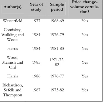
”It takes volume to move prices” is a common saying on the world’s stock exchanges. We wish to shed light on the fact that trading volume can explain price movements and thus have a very important role on financial markets. However, the causality in the price-volume relationships is an ambiguous matter in financial research. The price-volume phenomenon is a subject that attracts a lot of research and there are numerous studies that report a posi-tive correlation between the absolute price change and the trading volume. Table 2.1 is a synthesis of important results. All studies were made on stocks.

Table 2.1. A synthesis of important result on price-volume correlations (Source: Karpoff, 1987)

Author(s) Year of _study Sample _period volume correla-Price change-tion? Westerfield 1977 1968-69 Yes Comiskey, Walkling and Weeks 1984 1976-79 Yes Harris 1984 1981-83 Yes Wood, Mcinish and Ord 1985 1971-72, 82 Yes Harris 1986 1976-77 Yes Richardson, Sefcik and Thompson 1987 1973-82 Yes

There exist four theoretical explanations to this relationship. They are: The sequential arri-val of information (SAI) model, the mixture of distributions (MD) model, the rational ex-pectation asset pricing (REAP) model, and the differences of opinion (DO) model (Chen, 2001). The SAI model which was originally invented by Copeland (1976) has been devel-oped by Barry and Jennings (1983) and others. In the new version, new information is spread out to traders sequentially. The traders who are not yet informed do not perfectly know if they are trading against informed counterparts. Consequently, this sequence of new information distribution will generate both trading volume and price movements; both will increase in times of information shocks.

In the MD model, developed by Epps and Epps (1976) both price movements and trading volume depend the same variable, which can be interpreted as the rate of information flow

to the market. This suggests that both volume and price movements change together to new information (Chen, 2001).

In Wang’s (1994) REAP model the uninformed are trading against the informed and are facing adverse selection. Because of this a premium is demanded by the uninformed. For a given size trade the price has to adjust more than would be the case if they had the same in-formation with the result that the correlation between volume and price changes increases in information asymmetry.

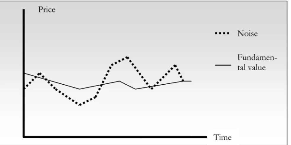
3.2 Noise

To further explain the relationship between the trading volume and information asymmetry it is important to consider noise in the market. Uninformed investors are also referred to as noise traders. Black (1986) states that noise can be viewed as signals about a stock’s value or future dividend that can be mistaken for information. The noise part of the price is the difference between the price and the fundamental value. It is the part of the price that is not information, e.g. a sharp fall in the main index that affects other stocks as well. How-ever information can be just noise itself if it is already discounted in the price. It is hard to estimate fundamental value because all estimates of it are noisy themselves, so one can never know how far from fundamental value the price is. The volatility of price, in the short term, will be greater than the volatility of fundamental value but in time horizons over several years the volatility will converge because price tends to return to the funda-mental value.

Figure 2.2, Simplified description of noise Price

Noise Fundamen-tal value

Time

Black further states that the noise affects the financial markets, making them possible, but also imperfect. Noise provides liquidity to financial markets but it is also putting noise to prices, making it hard to estimate actual value. Noise trading is trading on noise as if it were information. From an objective point of view noise traders would be better of not trading, than trading on the noise.

Noise trading creates an opportunity for informed investors to take advantage of. With many noise traders on the market it will pay off to gather information to trade on. It even pays off to gather costly information. In this situation, as a group, noise traders will lose money and informed traders will make money.

The information traders will trade with noise traders more than with other informed trad-ers, therefore cutting back in noise trading has the same effect on information trading. The effect on noise and trading volume is shown by Wang (1994). By increasing noise in public signals, the signal becomes less informative and information asymmetry increase be-tween the two classes. This will reduce trading volume since the uninformed trader will have less information and trade less on average.

3.3

Trading volume in information asymmetries

Here we give a review of theoretical models on trading volume in information asymmetries. This is our main theoretical framework and forms the basis for our hypotheses. The first two sections discuss the behavior of trading volume in information asymmetries. Our as-sumption is, based on Chae (2005) that around scheduled corporate announcements the in-formation asymmetry much more severe than normal. The last section discusses trading volume around unscheduled announcements, when uninformed investors are unprepared.

3.3.1 Trading volume prior to scheduled announcements

Wang (1994) developed a model to study the relation between trading volume and return. The model gives an explanation how information affects trading volume. It is based on a simple economy with both traded assets and private investment opportunities. The differ-ent investors in the market have differdiffer-ent private investmdiffer-ent opportunities and differdiffer-ent information about the stocks future dividends. The informed investors have private infor-mation whereas the uninformed investors get inforinfor-mation from realized dividends, price and public signals to determine future dividends. Informational trading arises when the in-formed investors receive private information and trade while the noninformational trading is when they trade to optimally rebalance their portfolio. The uninformed investors trade only for noninformational reasons. Since not all trade from the informed investors are in-formation motivated, the uninformed investors are willing to trade at favorable prices and expect to earn abnormal future returns. Since the uninformed investors can not perfectly identify the incentives of their counterpart they face the risk of trading against private in-formation. Because of this, as the information asymmetry between the two groups of inves-tors increase, trading volume will decrease since the adverse selection problem worsens. Furthermore, under asymmetric information, public news about a stock’s future dividends causes abnormal trading. The different in response to the same information by the two classes of investors generates trading. The greater the information asymmetry, the larger the abnormal trading volume when public news arrives.

Foster and Wiswanathan (1990) describe a model where there is one informed investor with monopoly on information, a group of uninformed investors and a market maker. Trading is spread out on days of the week. Informed investors receive informative signals about the stock’s future payoffs, whereas the uninformed investors only get a noisy public signals. The advantage of the informed investor is reduced through time by public informa-tion and the market maker’s price responses to order flow. It is assumed that the market maker adjusts the price responses when she faces adverse selection. The more sensitive the prices are to order flow the higher are the transaction costs for all investors. They argue that, because the price is important information for uninformed investors, the longer the market is closed the greater is the advantage for informed investors with private informa-tion. Thus, after the weekend, on Mondays, is the advantage the greatest of the week. The market maker has adjusted price responsiveness to orders to its highest on Mondays

be-cause the informed investor has gathered information during the weekend which has given her an even greater advantage.

This leads to a situation where the transaction costs for all investors in this game is highest on Mondays when the adverse selection is the greatest of the week. This reduces trading volume significantly. Also, they provide a theorem that says that without an earnings report in the week, the market maker’s responsiveness of prices to order flow declines over the week, reflecting that the market maker assumes that the information asymmetry is not so great. For weeks with a report, prices are more sensitive to order flow prior to the report, making it more costly to trade. The sensitivity of prices is reduced after the report is re-leased and it gets cheaper to trade.

Kyle (1985) came to another conclusion in his model on private information and trading. As information asymmetry increase, so does trading volume. The informed investors use their information in an attempt to exploit the market. The study differs from Wang’s in the sense that quantity has not a remarkable affect on the price and uninformed investors lack timing discretion.

3.3.2 Trading volume after scheduled announcements

In George et. al. (1994) a model with uninformed investors, informed investors and a spe-cialist who has monopoly on setting the bid and ask prices of a risky asset. The spespe-cialist sets his prices so as to maximize her profits. A wider bid-ask spread increases the transac-tion costs for all investors. An increase in informatransac-tion asymmetry increases the size of the informed investors order because then, her advantage would be greatest. It is showed that the greater the information asymmetry between the specialist and the informed investors the bigger are the specialist’s expected losses from trading the security. In response, the specialist widens the bid-ask spread during periods when she expects heavy trading by in-formed investors. When this happens, the uninin-formed investors will decrease their trading. The responsiveness of equilibrium trading volume to changes in information asymmetries depends on the pattern of uninformed trading. In an information asymmetry when the in-formed investors increase their trading, the specialist widens the bid-ask spread. If the net outcome is a decrease or an increase in total trading volume depends on whether unin-formed trading decreases in a decreasing or an increasing rate. If the rate is decreasing then the relatively little trading is discouraged by an increase in the spread. This makes the spe-cialist set the spread even wider in response to extreme information asymmetries, which in turn decreases total trading volume. This has the important implication that, when the in-formation asymmetry is resolved, as would be the case after an earnings announcement, the transaction costs would be significantly lower. This induces uninformed investors to trade and the effect would be an increase in total trading volume.

Foster and Wiswanathan (1990) propose that Friday is the day of the week with highest trading volume, simply put, because uninformed investors have gathered information dur-ing the week and Friday is therefore the day with the lowest information asymmetry. This reflects the fact that trading volume increases once the information asymmetry is resolved, as would be the case after scheduled announcements.

3.3.3 Trading volume around unscheduled announcements

The former models imply a decrease in trading volume prior to scheduled public an-nouncements. We assume, like Chae (2005), that for unscheduled announcements, it gets

impossible for uninformed investors to predict informed trading and hence are unable to adjust their own trading accordingly. The informed traders are eager to exploit their advan-tage and increase their trading. When the uninformed investors trade as usual and the in-formed investors increase their trading the outcome would be an increase in total trading prior to unscheduled public announcements.

3.4

Critique of the theoretical framework

Kyle’s (1985) model has a fundamental flaw; it assumes that uninformed investors have no discretion of when to place their trades which is a bit harsh, it must be that uninformed traders can select strategically when to place their trades.

A clear enhancement of this model was developed by Foster and Wiswanathan (1990) where they introduced continuous trading days and allowed new information to enter the market each day. The model also assumes that there is only one informed investor which gives the model a bit nondynamic features. Also it is argued that the implications of the model mean that the decrease in volume should be greater for bigger, more actively traded stocks, opposing the theory stating that information asymmetries are greater for “riskier” stocks (firm size often function as a proxy for risk). This model is also non-competitive, it only assumes that there is an investor with superior knowledge that she is trying to exploit strategically.

Both Kyle and Foster and Wiswanathan and Geroge et. al. (1994) assume that there exists a market maker. The role of the market maker is to warrant trading in a security by providing bid-ask spreads. In Sweden, only the smallest stock indices like “Nya marknaden” and “NGM” practice market making so in practice a model that assumes a market maker is not the most relevant on a larger stock index, however the main aspects of it are still applica-ble.

Wang’s (1994) model does include the role of the market maker. It also includes competi-tive trading where everyone is trying to maximize their profits. It also models both infor-mational and noninforinfor-mational trading as investors’ optimizing behavior, whereas the first three models model noninformational trading as liquidity trading without determining its economic origin. The main drawback of Wang’s model is that there are no transaction costs involved, every investor is free to do as many trades as she wants which encourages an abnormal trading activity.

4 Previous

Studies

Previous studies relevant to our own thesis is presented in the following chapter. We will use our own hy-potheses to present the findings in earlier research.

4.1

Trading Volume, Information Asymmetry, and Timing

In-formation

Joon Chae (2005), Journal Article

There have been quite a few theoretical models developed in the field of information asymmetry and abnormal trading volume. The ones that are relevant to our study are men-tioned in the previous chapter. Yet, there has only been one article written that study trad-ing volume around scheduled and unscheduled announcements. Below follows a presenta-tion of the thesis our study is based on.

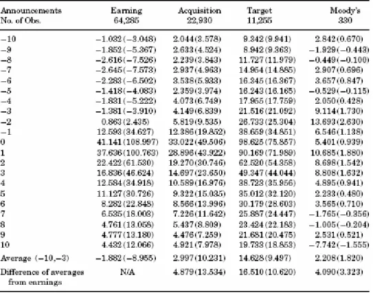
Chae’s study was carried out using earnings-, acquisition- and Moody’s announcements, all from New York Stock Exchange (NYSE) and American Stock and Option Exchange (AMEX) companies.. The time period studied was 1986 to 2000. Chae’s results are pre-sented in table 4.1. Each value is in abnormal log turnover the same measurement as we use. Respective t-value is presented in parenthesis.

Table 4.1. Daily Abnormal Turnover around Different Events. T-value in parenthesis (Source: Chae, 2005)

ƒ Hypothesis 1: The trading volume decreases before a scheduled announcement. A scheduled announcement refers to an announcement for which the public know the spe-cific date it will be released. Chae used earnings announcements as scheduled announce-ments. The result of the study was that cumulative trading volume decrease by more than 15 percent before scheduled announcements. He found that there was a relationship be-tween trading volume and information asymmetry. The findings were consistent with the theories of asymmetric information. As uninformed traders are facing high adverse selec-tion costs, they decrease their trading.

ƒ Hypothesis 2: There is a corresponding increase in trading volume after the

scheduled announcement is released.

Consistent with the first hypothesis, Chae found that trading volume increased after a scheduled announcement. Abnormal turnover in trading volume was significant each of the days following a scheduled announcement. This is evidences that uninformed investors time their trades and the decrease in trading volume before the announcement is the amount of delayed trading. Uninformed investors make up for their delayed trading once the information is released.

ƒ Hypothesis 3: The trading volume increases before an unscheduled

announce-ment.

Unscheduled announcements refers to an announcement for which the public do not know the date it will be released. Chae used acquisition, target and Moody’s bond rating an-nouncements for unscheduled anan-nouncements. The findings were that trading volume be-fore unscheduled announcements increased. By comparing this result to the result bebe-fore a scheduled announcement, Chae showed that the uniformed investors have no chance to time their trade around an unscheduled announcement. The increase in trading volume be-fore unscheduled announcements indicates that the informed investors exploit their advan-tage in information.

ƒ Hypothesis 4: All the assumed effects are greater for the firms on O-listan. When doing regressions Chae found that there was a relation between firm size and the behavior of trading volume for scheduled announcements. On the other hand, size was not positively related to trading volume before either of the unscheduled announcements. Chae argues that, if the argument that information asymmetry is greater for smaller companies is accepted, then these results imply that information asymmetry affects trading behavior only before scheduled announcements.

5 Empirical

findings

In the following chapter we will present the results from the statistical tests described in Chapter 2. First we will present our Preliminary studied and then move on to show the result for our Main study. A robustness test will also be reported for in this chapter. The empirical findings along with the theoretical framework will be used further in Chapter 6, the analysis.

5.1 Preliminary

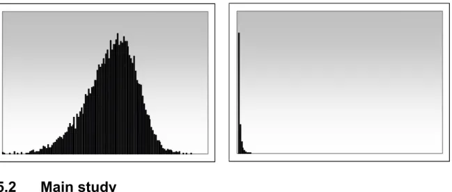
study

We performed a preliminary study to check our turnover data both on a normal scale and on a log scale. The result showed extreme skewness and kurtosis without log. As shown in table 5.1., by using log on the turnover we reduced skewness and kurtosis significantly. This resulted in a much more normally distributed sample as presented visually by the histo-grams in figure 5.1. This result is close to a normal distribution and therefore a log scale is used in our statistical testing.

Table 5.1. Descriptive statistics from preliminary study.

Period Mean SD Skewness Kurtosis Daily Turnover 1998-2004 0,0029 0,0063 21,637 987,713

Log Daily Turnover 1998-2004 -2,9531 0,6810 -0,802 1,388 Figure 5.1, Histogram for log turnover (left) and non log turnover (right)

5.2 Main

study

We present the abnormal log turnover for each day around the announcement in table 5.2. In parenthesis is the t-value obtained by the paired-samples t-tests.

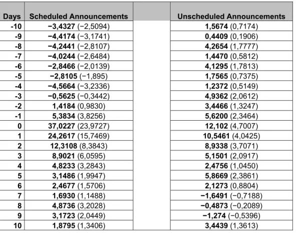
Table 5.2. Daily Abnormal Turnover around Different Announcements

Days Scheduled Announcements Unscheduled Announcements -10 −3,4327 (−2,5094) 1,5674 (0,7174) -9 −4,4174 (−3,1741) 0,4409 (0,1906) -8 −4,2441 (−2,8107) 4,2654 (1,7777) -7 −4,0244 (−2,6484) 1,4470 (0,5812) -6 −2,8466 (−2,0139) 4,1295 (1,7813) -5 −2,8105 (−1,895) 1,7565 (0,7375) -4 −4,5664 (−3,2336) 1,2372 (0,5149) -3 −0,5625 (−0,3442) 4,9362 (2,0612) -2 1,4184 (0,9830) 3,4466 (1,3247) -1 5,3834 (3,8256) 5,6200 (2,3464) 0 37,0227 (23,9727) 12,102 (4,7007) 1 24,2617 (15,7469) 10,5461 (4,0425) 2 12,3108 (8,3843) 8,9338 (3,7071) 3 8,9021 (6,0595) 5,1501 (2,0917) 4 4,8233 (3,2843) 2,4756 (1,0450) 5 3,1486 (1,9947) 5,8669 (2,3861) 6 2,4677 (1,5706) 2,1273 (0,8804) 7 1,6930 (1,1488) −1,6491 (−0,7188) 8 4,8736 (3,2028) −0,4873 (−0,2089) 9 3,1723 (2,0449) −1,274 (−0,5396) 10 1,8795 (1,3406) 3,4439 (1,3613) 5.2.1 Scheduled announcements

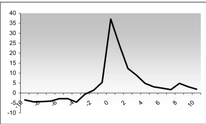
As shown in table 5.2. there is a decrease compared to benchmark from day -10 to day -3 with around -2.5 to -4.5 percent in log terms. This corresponds to a decrease in non log terms of 5-10 percent. There is a statistically significant decrease in turnover from day -10 to day -4 on a .05 significance level except for day -5, which is significant on a .10 signifi-cance level. Notably, as demonstrated in table 5.2 and in figure 5.2 the turnover is getting lower and lower from day -10 to day -8 to then increase slightly up to the days just prior to the announcement. To summarize, there is a statistically significant decrease on 6 of the 10 days prior to the announcement is released.

Figure 5.2.1, Turnover around scheduled announcements -10 -5 0 5 10 15 20 25 30 35 40 -10 -8 -6 -4 -2 0 2 4 6 8 10

On day 0, the turnover is increasing drastically, a log abnormal turnover of 37.02 which is equal to a non log increase of 134.5 percent. In the following days, the increase is declining but is statistically significant until day 5. Interesting is the sudden increase on day 8 and 9. On both days is the increase statistically significant. We report a statistically significant in-crease in turnover on 7 of the 10 days after the announcement.

5.2.2 Unscheduled announcements

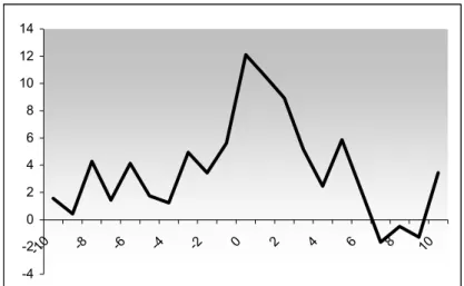
There is a clear difference in turnover before unscheduled announcements and scheduled announcements. Instead of a negative abnormal turnover before information being re-leased as in the case of scheduled announcements, here we observe a positive abnormal turnover. Trading volume is on average 2.88 percent higher than normal in log term be-tween day -10 and day -1. This corresponds to an average 6.87 percent increase in turnover in non log terms. The positive turnover between day -10 and day -4 is not statistically sig-nificant, even on a .1 sig. level, except for day -8 and day -6. We observe statistical signifi-cant turnover on day -3 and day -1. After the information is released the trading volume in-creases and from day 0 to day 3 we have a statistically significant abnormal turnover. On day 0, the turnover increases by 32 percent in non log terms. Except for day 5 we can not see statistical evidence of any abnormal turnover and from day 7 to day 9 we observe a small decrease in the turnover.

Figure 5.2.2, Turnover around scheduled announcements -4 -2 0 2 4 6 8 10 12 14 -10 -8 -6 -4 -2 0 2 4 6 8 10

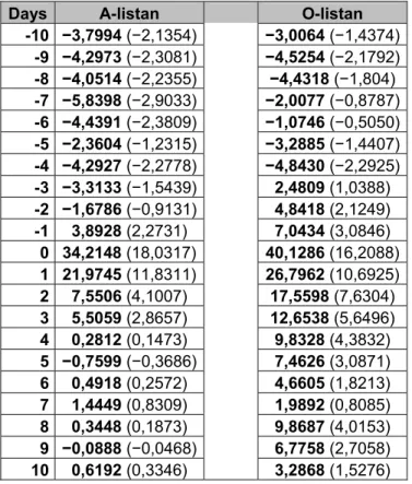
5.3

Comparison A-listan and O-listan

5.3.1 Scheduled Announcement

By observing figure 5.3. it can be concluded that the pattern of turnover is behaving similar for the two indices. Before the release of the announcement the decrease is greater for stocks on A-listan with an average decrease from day -10 to -4 of -4.15 in log terms which is the same as a normal decrease of 9.12 percent. O-listan is has an average decrease (-10 to -4) of -3.31 in log terms, corresponding to -6.91 percent in normal terms. In this period, the decrease is statistically significant for 6 days for A-listan in contrast to 3 days for O-listan.

As seen in figure 5.3, after the announcement is released in seems that the increase is greater for O-listan. A-listan has an average increase from day 0 to day +6 of 9.89 in log terms (25.57 percent non log) compared to the average increase of O-listan of 17.01 in log terms (47.96 percent non log). For O-listan, the increase is statistically significant for all days in the mentioned period but only for 4 days for A-listan.

Table 5.2. Daily Abnormal Turnover around scheduled announcements for A- and O-listan

Days A-listan O-listan -10 −3,7994 (−2,1354) −3,0064 (−1,4374) -9 −4,2973 (−2,3081) −4,5254 (−2,1792) -8 −4,0514 (−2,2355) −4,4318 (−1,804) -7 −5,8398 (−2,9033) −2,0077 (−0,8787) -6 −4,4391 (−2,3809) −1,0746 (−0,5050) -5 −2,3604 (−1,2315) −3,2885 (−1,4407) -4 −4,2927 (−2,2778) −4,8430 (−2,2925) -3 −3,3133 (−1,5439) 2,4809 (1,0388) -2 −1,6786 (−0,9131) 4,8418 (2,1249) -1 3,8928 (2,2731) 7,0434 (3,0846) 0 34,2148 (18,0317) 40,1286 (16,2088) 1 21,9745 (11,8311) 26,7962 (10,6925) 2 7,5506 (4,1007) 17,5598 (7,6304) 3 5,5059 (2,8657) 12,6538 (5,6496) 4 0,2812 (0,1473) 9,8328 (4,3832) 5 −0,7599 (−0,3686) 7,4626 (3,0871) 6 0,4918 (0,2572) 4,6605 (1,8213) 7 1,4449 (0,8309) 1,9892 (0,8085) 8 0,3448 (0,1873) 9,8687 (4,0153) 9 −0,0888 (−0,0468) 6,7758 (2,7058) 10 0,6192 (0,3346) 3,2868 (1,5276)

Figure 5.3. Comparison A-listan/O-listan, Scheduled announcements.

-10 0 10 20 30 40 50 -10 -8 -6 -4 -2 0 2 4 6 8 10 A-listan O-listan 5.3.2 Unscheduled Announcements

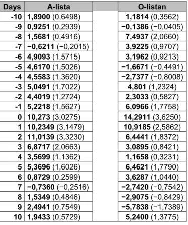
Here we observed an average increase day -10 to day -4 of 2.55 log terms (6 percent non log) for A-listan and an increase of 1.61 log terms ( 3.77 percent) for O-listan. However, the results are very weak, for A-listan none of the days in this period is statistically signifi-cant and only 1 day is signifisignifi-cant for O-listan.

Table 5.2. Daily Abnormal Turnover around scheduled announcements for A- and O-listan

Days A-lista O-listan -10 1,8900 (0,6498) 1,1814 (0,3562) -9 0,9251 (0,2939) −0,1386 (−0,0405) -8 1,5681 (0,4916) 7,4937 (2,0660) -7 −0,6211 (−0,2015) 3,9225 (0,9707) -6 4,9093 (1,5715) 3,1962 (0,9213) -5 4,6170 (1,5026) −1,6671 (−0,4491) -4 4,5583 (1,3620) −2,7377 (−0,8008) -3 5,0491 (1,7022) 4,801 (1,2324) -2 4,4019 (1,2724) 2,3033 (0,5827) -1 5,2218 (1,5627) 6,0966 (1,7758) 0 10,273 (3,0275) 14,2911 (3,6250) 1 10,2349 (3,1479) 10,9185 (2,5862) 2 11,0139 (3,3230) 6,4441 (1,8372) 3 6,8717 (2,0663) 3,0895 (0,8421) 4 3,5699 (1,1362) 1,1658 (0,3231) 5 5,3696 (1,6026) 6,4621 (1,7790) 6 0,8729 (0,2599) 3,6287 (1,0440) 7 −0,7360 (−0,2516) −2,7420 (−0,7542) 8 1,5349 (0,4846) −2,9075 (−0,8429) 9 2,4941 (0,7549) −5,7838 (−1,7389) 10 1,9433 (0,5729) 5,2400 (1,3775)

5.4 Robustness

check

To check for robustness in our results we performed a second test using different days as a benchmark. The benchmark was set as the average log turnover from day -20 to day 10. The results from the tests are summarized in table 5.3.

Table 5.3. Robustness test: Daily Abnormal Turnover around Different Announcements

Days

Scheduled Announcements Unscheduled Announcements -10 −5,4181 (−4,2985) −1,6373 (−0,8275) -9 −6,4027 (−5,1788) −2,7638 (−1,3619) -8 −6,2295 (−4,5185) 1,0607 (0,4804) -7 −6,0097 (−4,4767) −1,7576 (−0,8392) -6 −4,8319 (−4,0072) 0,9248 (0,4740) -5 −4,7995 (−3,6233) −1,4482 (−0,7133) -4 −6,5517 (−5,2939) −1,9676 (−0,9260) -3 −2,5478 (−1,7693) 1,7314 (0,8936) -2 −0,5669 (−0,4411) 0,2419 (0,1099) -1 3,3981 (2,7702) 2,4153 (1,2403) 0 35,0373 (26,9668) 8,8973 (4,0623) 1 22,2764 (17,295) 7,3414 (3,3852) 2 10,3254 (8,2259) 5,729 (2,7306) 3 6,9167 (5,4546) 1,9453 (0,9383) 4 2,8379 (2,1883) −0,7292 (−0,3793) 5 1,1632 (0,8492) 2,6622 (1,2685) 6 0,4824 (0,3417) −1,0774 (−0,5366) 7 −0,2923 (−0,2270) −4,8539 (−2,6148) 8 2,8883 (2,1236) −3,692 (−1,8259) 9 1,1869 (0,8506) −4,4787 (−2,3298) 10 −0,1285 (−0,1027) 0,2392 (0,1104) 5.4.1 Scheduled announcements

Using the different set of data in the robustness test resulted in an even stronger relation-ship the days before a scheduled announcement. The turnover is lower than average from day -10 to day to day -2. The abnormal turnover is statistically significant from day -10 to day -4, using a .05 sig level. Day -3 becomes significant using a .10 sig. level. Between these days, the decrease in log turnover is between 2.5 and 6.5 percent which correspond to a 6 to 16 percent decrease in non log terms. Summarizing the days before scheduled an-nouncements in the robustness test, we find that abnormal turnover is statistically signifi-cant in 8 of the 10 days.

The day 0 log turnover is 35 percent and this increase is equal to 124 percent in non log numbers. After the information is released the increase is declining and we can observe negative turnover on day 7 and day 10. Consistent with the main study, the turnover sud-denly increase on day 8. There is a significant abnormal turnover present in 5 of the 10 days after the announcement.

5.4.2 Unscheduled Announcements

The result from the robustness test also shows a clear difference in turnover between scheduled announcements and unscheduled announcements. By using the new benchmark on the unscheduled announcements, the days before company information is being re-leased show no statistically significance in turnover. An interesting observation one can make is that the increase/decrease in turnover between the days are the same as in the main study, the numbers in the robustness test is just lower.

Day 0 the turnover increases significantly with 22.7 in non log terms. We also observe ab-normal turnover with statistically significance on day 1 and day 2. After this, turnover is de-clining and we observe no abnormal turnover the next couple of days. From day 7 to day 9 there is a negative abnormal turnover present that is statistically significant on 0.10 sig. level.

6 Analysis

In this chapter we will compare the result of the study with earlier relevant studies. Further, we will use a critical approach to discuss the results relation to the theory presented in chapter 3. This chapter is related to the problem and will be further used in the next chapter, Conclusion and final discussion

6.1

Comparison of studies

Since there exists only one earlier study directly related to ours we compare our results to those found by Chae (2005). We will not compare our comparison between A-listan and O-listan to any of his result. This is due to the fact that our method differed considerably from his. As seen in figure 6.1. our results are close his. The main difference is that he found a statistically significant abnormal turnover on each of the 21 days studied. This is probably due to the significantly larger sample. We found a statistically significant decrease in turnover on 6 of the 10 days before a scheduled announcement is released, with a larger decrease on the days -10 to -3.

After the announcement is released we found a statistically significant increase on 7 of the 10 days. The turnover in Chae’s study is, on average, higher than ours after day 0 with a smoother decline.

Figure 6.1, Comparison of studies around scheduled announcements

-10 0 10 20 30 40 50 -10 -9 -8 -7 -6 -5 -4 -3 -2 -1 0 1 2 3 4 5 6 7 8 9 10 Johansson & Wilandh, 2005 Chae, 2005

The difference is larger in the case of unscheduled announcements. As shown in figure 6.2 the overall shape of the turnover pattern is roughly the same but ours is pointier with much lower increase just before day 0. Both studies reported an increase in turnover before day 0 but, as opposed to ours, Chae again observed a statistically significant increase on all days studied. The two studies report positive abnormal turnover prior to day 0 but we were only able to statistically justify the increase on 4 of the 10 days. After the announcement we ob-served a significant increase on 4 days.