An integrative approach to inventory control

http://www.diva-portal.org

Postprint

This is the accepted version of a paper presented at The Rapid Modeling Conference, Neuchâtel, June 30-July 1, 2009..

Citation for the original published paper:

Hedenstierna, P., Hilletofth, P., Hilmola, O-P. (2009) An integrative approach to inventory control.

In: Gerald Reiner (ed.), Rapid Modelling for Increasing Competitiveness : Tools and Mindset: Proceedings of the 1st Rapid Modeling Conference (pp. 105-118). Springer

https://doi.org/10.1007/978-1-84882-748-6_9

N.B. When citing this work, cite the original published paper.

Permanent link to this version:

Proceedings of the 1st Rapid Modeling Conference (Neuchâtel, Switzerland)

An integrative approach to inventory control

Philip Hedenstierna1, Per Hilletofth1*, and Olli-Pekka Hilmola2

1 _{Logistics Research Group, University of Skövde, 541 28 Skövde, Sweden}

2 _{Lappeenranta Univ. of Tech., Kouvola Unit, Prikaatintie 9, 45100 Kouvola, Finland}

Abstract

Inventory control systems consist of three types of methods: forecasting, safety stock sizing and order timing and sizing. These are all part of the interpretation of a planning environment to generate replenishment orders, and may consequently affect the performance of a system. It is therefore essential to integrate these aspects into a complete inventory control process, to be able to evaluate different methods for certain environments as well as for predicting the overall performance of a system. In this research a framework of an integrated inventory control process has been developed, covering all relations from planning environment to performance measures. Based on this framework a simulation model has been constructed; the objective is to show how integrated inventory control systems perform in comparison to theoretical predictions as well as to show the benefits of using an integrated inventory control process when evaluating the appropriateness of inventory control solutions. Results indicate that only simple applications (for instance without forecasts or seasonality) correspond to theoretical cost and service level calculations, while more complex models (forecasts and changing demand patterns) show the need for tight synchronization between forecasts and reordering methods. As the framework describes all relations that affect performance, it simplifies the construction of simulation models and makes them accurate. Another benefit of the framework is that it may be used to transfer simulation models to real-world applications, or vice versa, without loss of functionality.

1. Introduction

The purpose of inventory control is to ensure service to processes or customers in a cost-efficient manner, which means that the cost of materials acquisition is balanced with the cost of holding inventory [1]. This is done by interpreting data describing the planning environment, i.e. the parameters that may affect the

* Corresponding author: Tel.: +46 (0)500 44 85 88; Fax: +46 (0)500 44 87 99; E-mail: per.hilletofth@his.se

decision, to generate replenishment order times and quantities [2] (a breakdown of parameters is shown in [3]). The performance of an inventory control system may then be measured by the service and the total cost caused, when applied in a certain environment. Inventory control methods may be classified by whether they determine ordering timing, quantity, or both [3]. For systems that determine only one aspect, such as the reorder point system or the periodic ordering system, the undetermined aspect must be calculated beforehand, typically using the economic order quantity or the corresponding economic inventory cycle time [4]. The parameters that inventory control systems are typically including such things as demand forecasts, projected lead times, holding rates and ordering costs. Of these, the forecast is of special concern, as it is not a part of the planning environment, but a product thereof. This makes forecasting, given our definition of inventory control, an integral part of the inventory control system. To maintain service when there is forecast and lead time variability, safety stock is used, which is based on variability and on the uncertain times relating to the used inventory control model [5]. As the safety stock incurs a holding cost, it may be argued that it should be part of the timing/sizing decision; however, it is usually excluded as optimization in most cases only gives insignificant cost savings [5]. However, in larger distribution systems reduction of safety stocks is one primary driver of centralization of warehouses to one location (e.g. demand pooling, square root law, see [6-7]) these could concern feeding warehouses of factories (e.g. [8]) as well as retail related distribution operations (e.g. [9]).

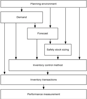
We have now discussed three interdependent areas that are usually treated individually. They are all part of the interpretation of the planning environment to generate replenishment orders, and may consequently affect the performance of the system. The current approach to inventory control does generally not consider it as a single system, but as separate methods (see e.g. Axsäter [5], Waters [4], Mattsson & Jonsson [3] and Vollman et.al [10]. An exception is Higgins [11], who describes inventory control as a process (see Fig. 1), but does not detail how information flows through the model, nor does he isolate the functions of forecasting, safety stock sizing and inventory control.

Looking at Higgins model, it is easy to realize that corruption of data occurring in an operation or between operations will cause the incorrect data to affect subsequent operations (see Ashby [12]). When theoretical models are applied to scenarios that follow the assumptions of the models, this is not an issue; but when a model is applied to a scenario it is not designed for, data corruption ensues. Applied to inventory control, this may mean that a simple forecast or a simple inventory control method is applied in an environment that does not reflect the method’s assumptions (The popularity of using simple methods, like the reorder point method is shown in [13] and [14]). When a method’s assumptions are unmet, its performance may be difficult to predict. The scenario of using theoretically improper methods is not unlikely, as businesses may want to utilize inventory control methods that are simple to manage, such as the reorder point system, even when the planning environment would require a dynamic lot-sizing method such as the Wagner-Whitin, Part-period or the Silver-Meal algorithm (see Axsäter [5]). In the same fashion, simple forecasting methods may be applied to

complex demand patterns to simplify the implementation and management of the forecasts.

Fig. 1. Higgins’ inventory control process model [7].

To understand how a method will respond to an environment it was not designed for, it is necessary to understand the entire process, from planning environment to measurement of results. As it may be difficult to predict how a system based on a required type of input will react to unsuitable data, a model of the system may help to give insight into the system’s performance. In his law of requisite variety, Ashby [12] states that a regulatory system must have at least as much variety as its input to fully control the outcome; applied to the inventory control process, this means that all aspects of a system must be modeled to get an accurate result. Inventory control systems consist of three types of methods: forecasting, safety stock sizing as well as order timing and sizing [5]. Though there are many individual methods, only one method of each type may be used in an inventory control system for a single stock-keeping unit.

In this research a framework of an integrated inventory control process has been developed, covering all relations from planning environment to performance measures. The design of the framework was based on a literature review of inventory control theory and on the authors’ experience of the area. Based on this framework a simulation model has been constructed considering demand aggregation, forecasting, and safety stock calculations, as well as reordering methods. The research objective of this study is to provide an increased understanding of the following research questions: (i) ‘How may the process of inventory control be described in a framework that allows for any combination of methods to be used?’, and (ii) ‘Is there any benefit of integrated inventory control when deciding appropriate inventory control solutions?’.

The remainder of this paper is structured as follows: First, Section 2 integrates existing theory to describe a framework for designing inventory control models. Section 3 introduces empirical data from a company, whose planning environment was interpreted in Section 4 to develop a simulation model based on the framework. Section 5 describes the results of the simulations. Thereafter, Section 6 discusses the implications of the results, while Section 8 describes the conclusions that can be drawn from the study.

2. Framework for integrated inventory control

The design of the framework is based on observing how inventory control methods operate, what input they require and what output they provide. An underlying assumption for inventory control systems is that there for any given time t, is an inventory level LL, which is reduced by demand D and increased by replenishment R. Another assumption is that time is divided into buckets (as described by Pidd [15]), for continuous systems buckets are infinitesimal, and that for each bucket the lowest inventory level, which is sufficient to evaluate the effects of inventory control, is governed by Formula 1. The relationship between these factors has been deduced from the rules that material requirements planning is built on [10]. t t t t

LL

R

D

LL

=

+

−

LL

where

LL

R

occurring before t and

D

Formula 1 dictates how transactions of any system placed in the framework will operate. It considers replenishment to occur between time buckets, meaning that it is sufficient to monitor the lowest inventory level to manage inventory transactions. Information such as service levels, inventory position and the highest stock level may be calculated from the lowest inventory level. The formula governs the inventory transactions of any inventory control system, and must be represented in any inventory control application. All other parts of an application may vary, either depending on the planning environment in which an inventory control system is used, or on the design of the system. Fig. 2 shows the framework, which starts with the planning environment and ends with a measurement of the system’s performance.

The planning environment comprises the characteristics of all aspects that may affect the timing/sizing decisions [2]. For each time unit, the environment, which determines the distribution of demand, generates momentary demand that is passed on to a forecasting method, to an inventory control method and to actual transactions. The type of demand, which is dictated by the planning environment, tells whether a backlog can be implemented or not, and what function that may represent it [4]. Forecasting is affected by past demand information and the planning environment [1]. The former is used to do time series analysis, which is common practice in inventory control, while the latter may concern other input, such as information that may improve forecasting or data needed for causal forecasting. The environment may also tell of changes in the demand pattern, which may necessitate adjusting forecasting parameters or changing the forecasting method. It is necessary to consider the aggregation level of data, as longer term forecasts will have a low coefficient of variation, at the cost of losing forecast responsiveness [10]. Forecast data is necessary for inventory control methods (forecasted mean values), and for safety stock sizing (forecast variability)

[4]. Safety stock sizing is a method buffering against deviations from the expected mean value of the forecast [4]. The assumption of safety stock sizing is that all forecasts are correct estimations of the future mean value of demand; any deviations from the forecast are attributed as demand variability. This effectively means that an ill-performing forecast simply detects higher demand variability than a good forecast. The sizing is also affected by the planning environment, as the uncertain time determines the need for safety stock, as lead times also may have variability, and as the environment will determine to what extent customers accept shortages, or low service [1].

Fig. 2. Framework describing relations within inventory control systems.

Inventory control methods rely on forecasts, on safety stock sizing and on the planning environment. The safety stock is used as a cushion to maintain service, while forecasts and data from the planning environment, which are ordering costs, holding costs and lead times, are used to determine when and/or how much to order [10]. The actual balancing of supply, which comes from the replenishment of the inventory, and demand, which is sales or lost sales, takes place as inventory transactions. Measuring these transactions gives an understanding of how well an inventory control system performs for the given planning environment [4].

3. Empirical data

Data was collected from a local timber yard, currently not using an inventory control policy. Existing functionality for the reorder point method and for the

periodic order quantity method allowed for these methods to be deployed at low cost. The issue was whether the methods could cope with the fluctuations in demand, as trend and seasonal components were assumed to exist. Based on an analysis of sales data, the demand for timber was found to be seasonal, but with no trend component. This information was used to generate a demand function, based on the normal distribution. The purpose of the demand function was to allow the simulation model to run several times (200 independent simulations of three consecutive years were run, with random seeds for each simulated day). Real demand, as well as a sample of simulated demand, is shown in Fig. 3.

Demand 0 1000 2000 3000 4000 5000 6000 7000 8000 9000 10000 1 3 5 7 9 11 13 15 17 19 21 23 25 27 29 31 33 35 Month Q u a n ti ty _{A c tual} S imulated

Fig. 3. Simulated and actual monthly demand.

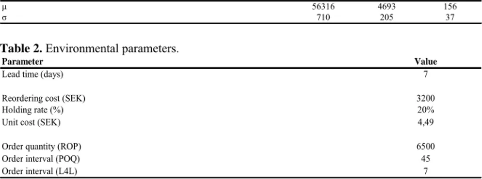
Demand characteristics are shown in Table 1 and other parameters pertaining to the planning environment are shown in Table 2. As transport costs were considered to be semi-fixed rather than variable, the reordering cost is valid for the reorder quantity used. Increasing the order quantity was not a cost-effective option. Stock out costs were not considered, as the consequences of stock outs are hard to measure; not only are sales lost, there is also the possibility of competitors winning the sale, and of losing customers, as they cannot find what they need.

Table 1. Demand characteristics.

Demand Year Month Day

μ 56316 4693 156

σ 710 205 37

Table 2. Environmental parameters.

Parameter Value

Lead time (days) 7

Reordering cost (SEK) 3200

Holding rate (%) 20%

Unit cost (SEK) 4,49

Order quantity (ROP) 6500

Order interval (POQ) 45

Lead times were considered as fixed, as no information on delivery timeliness was available. The expected fill rate (fraction of demand serviceable from stock) for the reorder point method was 99%, while the it for the periodic order quantity method would be 98% and for the lot-for-lot method would be 96% (calculated using the loss function, based on the standard deviation, as described by Axsäter [5]).

4. Simulation model

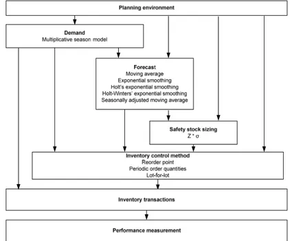
To test how the framework could be applied to a real-world scenario, a simulation model was constructed to evaluate inventory control solutions considered by a local timber yard. To support the inventory control systems, some simply managed forecasting systems were chosen. The complete selection of methods, put into the context of the framework is shown in Fig. 4.

Fig. 4. Methods placed in the framework.

All methods were verified against theory by testing, if the method implementations gave the values that theory dictates. For the reorder point method, the reorder point was raised by ½ days of forecasted demand, to prevent undershoot, as described in [16]. Several forecast methods were considered, and the actual choice of forecast for this case was based on the mean absolute deviation (See Table 3). Bias was calculated to see whether a forecasting method

followed the mean of demand. The seasonally adjusted moving average (see [4]) was chosen as the preferred method, as it proved to be nearly as accurate as Holt-Winters (see [1]), while not requiring as careful calibration.

Table 3. Summary of forecast errors.

Type EXP MA HOLT H-W S-MA

MAD 1281 1189 1267 179 263

Bias (%) 0,9% 0,3% 0,5% 0,1% -0,1%

Forecasts were monthly, and predicted the demand for the following month. The forecast value was multiplied by 1.5 to reflect an economic inventory cycle time of 45 days. This simplification was done to see how the system would react to systematic design errors.

5. Simulation results

To investigate how seasonality affects the performance of simple planning methods, variations of the presented demand pattern were simulated. In the first, demand was constant (Case 1); in the second, variance was added (Case 2), while in the third, seasonality (±20%) was introduced (Case 3). For the different cases a moving average forecast was used, adjusted for seasonality. Ignoring safety stock altogether, the measures used for the simulations were fill rate and inventory cycle service level. It should be noted that lot-for-lot has a different inventory cycle from the other reordering mechanisms, meaning that its service levels cannot be directly compared to them. Fig. 5 shows the results of the simulation runs.

0% 20% 40% 60% 80% 100% 1 2 3 Case C y cl e s e rvi c e l e v e l

Periodic order quantity Reorder point method Lot-for-lot 95% 96% 97% 98% 99% 100% 1 2 3 Case F ill r a

te Periodic order quantity

Reorder point method Lot-for-lot

What can be seen is that inventory cycle service is higher for the periodic order quantity method than for the reorder point method. However, the fill rate shows that the reorder point method is better at meeting demand. Together, the measures tell that the periodic order quantity method has fewer, but greater stock-outs than the reorder point method. Seasonality affected the fill rate of the periodic order method the worst, while the reorder point method was hardly affected.

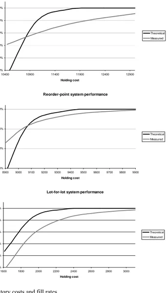
Periodic order system performance

95,0% 96,0% 97,0% 98,0% 99,0% 100,0% 10400 10900 11400 11900 12400 12900 Holding cost Fill r a te _Theoretical Measured

Reorder-point system performance

98,5% 99,0% 99,5% 100,0% 8900 9000 9100 9200 9300 9400 9500 9600 9700 9800 9900 Holding cost F ill r a te Theoretical Measured

Lot-for-lot system performance

95% 96% 97% 98% 99% 100% 1600 1800 2000 2200 2400 2600 2800 3000 Holding cost F ill r a te Theoretical Measured

Fig. 6. Total inventory costs and fill rates.

The final situation added the seasonal pattern of the original data, and considered another inventory control solution, namely lot-for-lot. The result is shown in Figure 6, which is the fill rate and the holding cost incurred, compared to

the theoretical fill rate, should no seasonality or forecast error be present. The periodic order quantity system shows a considerably worse fill rate than the reorder point system. The lot-for-lot system has a much lower holding cost than the other two methods due to more frequent orders; however, safety stock accounts for a larger fraction of the total holding, than for the other methods, leading to higher safety stock costs per stored unit. Observing the graphs, the lot-for-lot method is the only method where the measured cost/service relationship does not intersect with the theoretical function. For the methods with longer order cycles, the measured cost/service relationship shows a much flatter curve than expected, indicating that these functions will require more safety stock than expected to improve fill rates.

6. Discussion

Completed simulations indicate that the fill rate of the periodic order quantity method suffers when the seasonal demand pattern is introduced, while the reorder point method can maintain the same fill rate as if no seasonality were present. This is a result of the nature of the two methods, where variability affecting the reorder point method will affect the time of ordering, while the periodic order quantity method, with fixed ordering times, cannot regulate order timing to prevent stock outs. Instead, it must let the inventory level take the full effect of any variability. Conversely, the effect of variability on the reorder point method is that the resulting order interval may not be economic.

When comparing the methods used in the simulation using the framework, we find that the reorder point method is superior both concerning holding costs, and fill rate. What system is preferable depends on whether suppliers can manage to deliver varying quantities (up to three times the average, both for periodic ordering, and for lot-for-lot) or at varying intervals.

The difference between measured and theoretical fill rate demonstrated by the periodic order quantity shows how inventory control methods not designed for a certain planning environment can be affected. The use of a monthly forecast not representing the next inventory cycle may also have contributed to the low fill rate. The simulation based on the framework helped give insight into how the inventory control process would react to the planning environment. It showed that a large safety stock would be required if the periodic order quantity were to be used, as the periodic order quantity method undershot performance predictions much more than the reorder point method. If applied over multiple products, the framework can tell if consolidation using the sensitive periodic order quantity system is less costly than the reorder point system. Given that the periodic order quantity system has a 100% uncertain time [1], it may be used as a benchmark in simulations, as variability and problems caused by poor design of the process always are reflected in the fill rate.

In the future we plan to enlarge our simulation experiments by incorporating different kind of demand types (continuous and discontinuous) as well as new

methods used in forecasting and ordering. Recent research has shown that autoregressive forecasting methods outperform others in situations where demand is fluctuating widely and follows a “life-cycle” pattern [17]. Similarly, purchasing order method research argues that not a single ordering method should be used (so basically it is not a question, which method is the best one, but which one best suits the environment), but usually a combination of different purchasing methods should be incorporated in ERP systems during the entire life-cycle of a product [18]. However, if volumes are low, then even economic order quantities/reorder point systems, and periodic order policies should be abandoned; a lot for lot policy might produce best results in these situations [18]. Thus, much depends from the operations strategy (order or stock based system), and from the amount of time, which customers are willing to wait for a delivery to reach their facilities [19].

7. Conclusions

Treating inventory control and forecasting as separate activities, while not acknowledging how forecasting and its application affect inventory control may lead to incorrect assessments of a system’s performance in a certain planning environment. Approaching inventory control as a process, starting with a planning environment and ending with a measurement of the system’s performance shows that all activities are related, and that the end result may be affected by the activities or by the way they are connected. This paper uses a simulation model to show how the use of forecasts and complexity in demand patterns affects the performance of the reorder point system and the periodic order quantity system. Simulations show that performance generally is worse than expected, and that periodic ordering consistently shows a greater susceptibility both to variability and to design errors, due to its inability to buffer against these by changing the reordering interval. This weakness also appears in lot-for-lot systems, as they are based on periodic ordering.

References

[1] S. Axsäter: Lagerstyrning, Studentlitteratur, Lund, Sweden, 1991.

[2] S. A. Mattsson: Logistikens termer och begrepp, PLAN, Stockholm, Sweden, 2004. [3] S. A. Mattsson, and P. Jonsson: Produktionslogistik, Studentlitteratur, Lund, Sweden,

2003.

[4] D. Waters: Inventory Control and Management, Wiley, Hoboken, U.S.A., 2003. [5] S. Axsäter: Inventory Control, Springer, New York, U.S.A., 2006.

[6] W. Zinn, M. Levy, D., and J. Bowersox: “Measuring the effect of inventory centralization / decentralization on aggregate safety stock: The “square root law” revised”, Journal of Business Logistics, Vol. 10, No. 1, pp. 1-14, 1989.

[7] D. Chandrasekhar, and R. Tyagi: “Effect of correlated demands on safety stock centralization: patterns of correlation versus degree of centralization”, Journal of Business Logistics, Vol 20, No. 1, pp. 205-213, 1999.

[8] R. Lauri, and O.-P. Hilmola: “From manual to automated purchasing, case: middle-sized telecom electronics manufacturing unit”, Industrial Management and Data Systems, Vol. 105, No. 8, pp. 1053-1069, 2005.

[9] H.M. Leknes, and C. Carr: “Globalization, international configurations and strategic implications: the case of retailing”, Long Range Planning, Vol. 37, No. 1, pp.29-49, 2004. [10] T. E. Vollman, W. L. Berry, D. C. Whybark, and F. R. Jacobs: Manufacturing Planning

and Control for Supply Chain Management, McGraw-Hill, New York, U.S.A., 2004. [11] J. C. Higgins: Information systems for planning and control: concepts and cases, Edward

Arnold, London, United Kingdom, 1976.

[12] W. R. Ashby: An Introduction to Cybernetics, Chapman & Hall, London, United Kingdom, 1957.

[13] P. Jonsson and S.-A. Matsson: “A longitudinal study of material planning applications in manufacturing companies”, International Journal of Operations & Production Management, Vol. 26, No. 9, pp.971-995, 2006.

[14] A. Ghobbar and C. Friend: “The material requirements planning system for aircraft maintenance an inventory control: a note”, Journal of Air Transport Management, Vol. 10, pp. 217-221, 2004.

[15] M. Pidd: Computer Simulation in Management Science, Wiley, Hoboken, U.S.A., 1988. [16] S. A. Mattsson: “Inventory control in environments with short lead times”, International

Journal of Physical Distribution & Logistics Management, Vol.37, No.2, pp.115-130, 2007.

[17] S. Datta, C. W. J. Granger, D. P. Graham, N. Sagar, P. Doody, R. Slone, and O.P. Hilmola: “Forecasting and risk analysis in supply chain management – GARCH Proof of Concept”, MIT Forum for Supply Chain Innovation, ESDCEE, School of Engineering. Available at URL:

http://dspace.mit.edu/bitstream/handle/1721.1/43943/GARCH%20Proof%20of%20Conept %20_%20Datta_Granger_Graham_Sagar_Doody_Slone_Hilmola_%202008_December.p df?sequence=1. Retrieved: January 2009.

[18] O.-P. Hilmola, H. Ma, and S. Datta: “A portfolio approach for purchasing systems: Impact of switching point”, Massachusetts Institute of Technology, Engineering Systems Division Working Paper Series, ESD-WP-2008-07. Available at URL:

http://esd.mit.edu/WPS/2008/esd-wp-2008-07.pdf. Retrieved: January 2009.

[19] P. Hilletofth: “Differentiated Supply Chain Strategy – Response to a Fragmented and Complex Market”, Licentiate dissertation, Chalmers University of Technology, Department of Technology Management and Economics, Division of Logistics and Transportation, Göteborg, Sweden, 2008.