Gold During Recessions : A study about how gold can improve the performance of a portfolio during recessions

J

I

B

S

JÖNKÖPING UNIVERSITY

Gold During Recessions

A study about how gold can improve the performance of a portfolio during recessions

Bachelor Thesis in Business Administration Authors: Helmersson, Tobias

Kang, Hana Sköld, Robin Tutor: Österlund, Urban Jönköping December 2008

1

Acknowledgements

We would like to thank our tutor Mr. Urban Österlund for His insightful and enlightening comments and guidance. We would also like to give recognitions to Thomas Holgersson, Associate Professor in Statistics, and Agostino Manduchi, Assistant Professor in Financial Economics, both at Jönköping International Business School, for their valuable input and recommendations.

Finally, we are also grateful for all constructive inputs and comments from our fellow stu-dents during the seminar sessions.

Tobias Helmersson Hana Kang

Robin Sköld

Jönköping International Business School

2

Bachelor Thesis in Business Administration

Title: Gold During Recessions- A study about how gold improve the

performance of a portfolio during recessions.

Authors: Helmersson, Tobias

Kang, Hana Sköld, Robin

Tutor: Österlund, Urban

Date: December 2008

Subject terms: Gold, Recessions, Portfolio Allocation, Optimal Portfolio, Min-imum Variance Portfolio, Correlation, Return to Risk Ratio, DJIA.

Abstract

Problem: When choosing topic for this study the economy was on the brink of a recession. Many experts made varying statements regarding this fact, and further readings in this area led us to question: can an in-clusion of gold enhance the performance in an index portfolio dur-ing recessions? And if so, how much should be allocated to gold?

Purpose: The purpose of this thesis is to look back at the historical price de-velopment of gold and DJIA during recessions in order to find out whether an inclusion of gold can improve a DJIA index portfolio held in today’s recession. In addition, by analyzing the risks and pos-sibilities with gold, the optimal allocation of gold in a DJIA portfolio will be investigated in.

Method: The methodological approach will be of a quantitative data analysis approach. By using historical data, new empirical findings will be found by using the deductive approach. This method has been cho-sen due to the nature of the purpose and in order to best give a gen-eral answer to our research questions.

Conclusion: The gold price is strongly influenced by uncertainty, and even though an optimal allocation of gold in each recession could be found, no general optimal allocation applicable in today’s recession could be found. Gold has higher risk (higher variance) than DJIA, but is compensated with higher return as well.

3

Abbreviation Word List

DJIA = Dow Jones Industrial Average GDP= Gross Domestic Product OP = Optimal Portfolio

MVP = Mean Variance Portfolio CML= Capital Market Line

OPEC = Organization of the Petroleum Exporting Countries Today= 2008-2009

4

Table of Contents

3

Introduction ... 8

4

Frame of Reference ... 12

4.1 Economical theories and concepts ... 12

4.1.1 Business Cycles ... 12

4.1.2 Gold ... 14

4.1.2.1 Flow supply of gold ... 16

4.1.2.2 Demand of gold ... 18

4.1.2.3 Long Run ... 18

4.2 Financial theories ... 18

4.2.1 Uncertainty and Herd Behavior ... 18

4.2.2 Modern Portfolio Theory ... 19

4.2.2.1 Financial Statistical Section ... 19

4.2.2.2 Portfolio Theory Section ... 22

5

Historical Background ... 26

5.1 Dow Jones Industrial Average ... 26

5.2 Recessions ... 27

5.2.1 Recession 1 1973-11 – 1975-03 ... 27

5.2.1.1 Price movement of Gold Recession 1 ... 28

5.2.2 Recession 2 1980-01 – 1980-07 and Recession 3 1981-07 – 1982-11 ... 29

5.2.2.1 Price movement of Gold Recession 2 – Recession 3 ... 29

5.2.3 Recession 4 1990-07 – 1991-03 ... 30

5.2.3.1 Price movement of Gold Recession 4 ... 31

5.2.4 Recession 5 2001-03 – 2001-11 ... 32

5.2.4.1 Price movement of Gold Recession 5 ... 32

6

Method ... 34

6.1 Quantitative data collection ... 34

6.2 Deductive approach ... 34

6.3 Secondary data ... 35

6.4 Research process... 35

6.5 Collection of data ... 36

6.6 Use of Data ... 37

6.7 Criticism and Delimitations ... 38

6.7.1 Assumptions ... 38

7

Results and Analysis ... 40

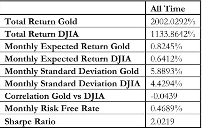
7.1 All time (1970 – 2008) ... 40

7.2 Recessions ... 43

7.2.1 Results and Analysis, Recession 1 (1973 – 1975) ... 44

7.2.2 Results and Analysis Recession 2 (1980 – 1980) ... 47

7.2.3 Results and Analysis, Recession 3 (1981 – 1982) ... 50

7.2.4 Results and Analysis Recession 4 (1990 – 1991) ... 53

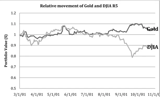
7.2.5 Results and Analysis Recession 5 (2001 – 2001) ... 56

5 7.4 Conclusive analysis ... 60

8

Conclusion ... 61

9

References ... 63

Figure 2 DJIA, Nov 07 – Sep 08 ... 8

Figure 3 FTSE 250 Index, Nov 07 – Sep 08 ... 8

Figure 4 Hang Seng Index, Nov 07 – Sep 08 ... 8

Figure 5 Price movement of gold 1970 - 2008 ... 9

Figure 6 Behavior of the components of GDP ... 13

Figure 7 Demand and Supply of Gold (World Gold Council) ... 15

Figure 8 Movement of Price of Gold and US Inflation 1972 - 2004 ... 16

Figure 9 World Gold Holdings 2006 ... 16

Figure 10 Total world mine production 1980 to 2004 Source: GFMS, Ltd. ... 17

Figure 11 Opportunity set of a portfolio ... 22

Figure 12 Return to risk ratio with different correlations ... 23

Figure 13 Efficient frontier, CML and the location of optimal portfolio ... 25

Figure 14 Correlation between S&P500 and DJIA 2008 ... 26

Figure 15 DJIA and Gold development during Recession 1 ... 28

Figure 16 DJIA and Gold development during recession 2 ... 30

Figure 17 DJIA and Gold development during Recession 3 ... 30

Figure 18 DJIA and Gold development during recession 4 ... 31

Figure 19 DJIA and Gold development during recession 5 ... 33

Figure 20 Deductive approach ... 35

Figure 21 MVP weights 1970 -2008 ... 42

Figure 22 OP weights 1970 - 2008 ... 42

Figure 23 Movement of DJIA, Gold and Optimal Portfolio, 1970 - 2008 ... 42

Figure 24 OP and MVP for Gold and DJIA on the Efficient Frontier 1970 – 2008 ... 43

Figure 25 MVP in Recession 1 ... 46

Figure 26 OP Recession 1 ... 46

Figure 27 OP and MVP for Gold and DJIA on the Efficient Frontier R1, 1973 – 1975 ... 46

Figure 28 Movements of Gold, OP, MVP and DJIA ... 47

Figure 29 MVP in Recession 2 ... 48

Figure 30 OP in Recession 2 ... 48

Figure 31 OP and MVP for Gold and DJIA on the Efficient Frontier R2, 1980 - 1980 ... 49

Figure 32 Movements of Gold, OP, MVP and DJIA 1980 - 1980 ... 50

Figure 33 MVP in Recession 3 ... 52

Figure 34 MVP for Gold and DJIA on the Efficient Frontier R3, 1981 – 1982 ... 52

Figure 35 Movement of Gold, MVP and DJIA 1981 – 1982 ... 53

Figure 36 MVP in Recession 4 ... 54

Figure 37 OP in Recession 4 ... 54

Figure 38 OP and MVP for Gold and DJIA on the Efficient Frontier R4, 1990 - 1991 ... 55

Figure 39 Movements of Gold, MVP and DJIA, 1990 - 1991 ... 55

Figure 40 MVP in Recession 5 ... 57

Figure 41 OP in Recession 5 ... 57

Figure 42 OP and MVP for Gold and DJIA on the Efficient Frontier R4, 2001 – 2001 ... 58

6

Tables

Table 1 All time data between 1970 – 2008, based on monthly data ... 40

Table 2 Allocations for Gold and DJIA with MVP and OP, 1970 - 2008 ... 41

Table 3 Overview of the Recessions ... 44

Table 4 Data for Recession 1 ... 44

Table 5 MVP and OP for Recession 1 ... 45

Table 6 Data for Recession 2 ... 47

Table 7 MVP and OP for Recession 2 ... 48

Table 8 Data for Recession 3 ... 50

Table 9 MVP for Recession 3... 51

Table 10 Data from Recession 4 ... 53

Table 11 MVP for Recession 4 ... 54

Table 12 Data for Recession 5 ... 56

Table 13 MVP and OP for Recession 5 ... 57

Table 14 Comparison of gold with other assets ... 59

Equations Equation 1 The return of an asset ... 19

Equation 2 Mean value of return ... 20

Equation 3 Expected return for a portfolio ... 20

Equation 4 Variance for an individual asset ... 20

Equation 5 Standard deviation for an individual asset ... 21

Equation 6 Covariance between two returns; RA and RB ... 21

Equation 7 Correlation coefficient between two assets ... 21

Equation 8 Variance of a portfolio ... 22

Equation 9 Weights for the minimum variance portfolio (MVP)... 23

Equation 10 Weights for the optimal portfolio (OP) ... 23

Equation 11 Return for the constructed portfolio ... 24

Equation 12 Variance for the constructed portfolio ... 24

Equation 13 Variance for the constructed portfolio ... 24

Equation 14 Standard deviation for the constructed portfolio ... 24

Equation 15 Capital market line ... 24

7

1 Disposition

Chapter 3 In this opening section, the background to the study will be presented where the specific

field of interest will be included. Further, the problem discussion followed by the specific re-search questions, the purpose and the approach will be stated.

Chapter 4 In this section, the related economical and financial concepts and theories will be presented. The main parts concern Business Cycles, Supply and Demand for Gold, and the Modern Portfolio Theory. In addition some other important definitions and equations will be in-troduced.

Chapter 5 As this study is based on historical data, it is important to have knowledge about the re-lated history. This part will present the reader with a brief introduction to DJIA and gold. After that, DJIA and gold development during each recession will be treated, togeth-er with graphical illustrations. Recession 2 and 3 are put togethtogeth-er due to the close connec-tion in time and possible shared causes and effects.

Chapter 6 In this part, our choice of the research method will be presented. Further on, our method for collecting and the manipulation of the data will be presented and the criticism against it, along with assumptions made for the analyses.

Chapter 7 This section presents the data collected and our findings. The data will be presented in

forms of tables and figures in order to give the reader an easy way of interpreting the find-ings. Parallel to the findings, the data and theory will be analyzed. At the end, gold will be compared to other assets, to see how it performs in relation to them.

Chapter 8 In this conclusive section, the findings from the study will be summarized together with the research questions. Further recommendations for future studies will also be presented.

8

2 Introduction

In this opening section, the background to the study will be presented where the specific field of interest will be included. Further, the problem discussion followed by the specific research questions, the purpose and the approach will be stated.

2.1 Background

George Santayana, a well-known philosopher, once expressed these words: “Those who cannot remember the past are condemned to repeat it.” (Reason in common sense)

As the quote above states, the history will repeat itself and it is therefore of vital impor-tance to analyze the past in order to pursue hints for the future. In today’s (2008) financial turmoil, the market has changed dramatically during a short period of time. Starting with the sub-prime mortgage crisis with falling house prices in the US, the world market is today under pressure to recover. Seemingly, history will repeat itself because people with self-fulfilling goals drive the market. Investors have lost large shares of their portfolio invest-ments and multinational companies and banks are struggling with their finances. The larg-est indexes all over the world have plummeted (see Figure 1-4) with 1-day record losses and the situation today is unstable, least to say.

Figure 1 Nikkei 225 Index, Nov 07 – Sep 08 Figure 2 DJIA, Nov 07 – Sep 08

Figure 3 FTSE 250 Index, Nov 07 – Sep 08 Figure 4 Hang Seng Index, Nov 07 – Sep 08 The downfalls that many countries have experienced this year (2008) have caught our at-tention, and it has made us question what there is to do in order to hinder even further losses for private investors. Are there any assets that could decrease the losses and perhaps even improve the portfolio performance? Gold has long been considered a safe haven in these circumstances, and in an article written by BBC News (2008-01) earlier this year in January, the gold price was on its way up, driven by the weak dollar, strong oil prices and global inflationary fears. In general, people perceive gold and other precious metal com-modities as lower risk investments, and with the fear of falling stock prices, people are now looking for various alternatives to safeguard their portfolios.

9

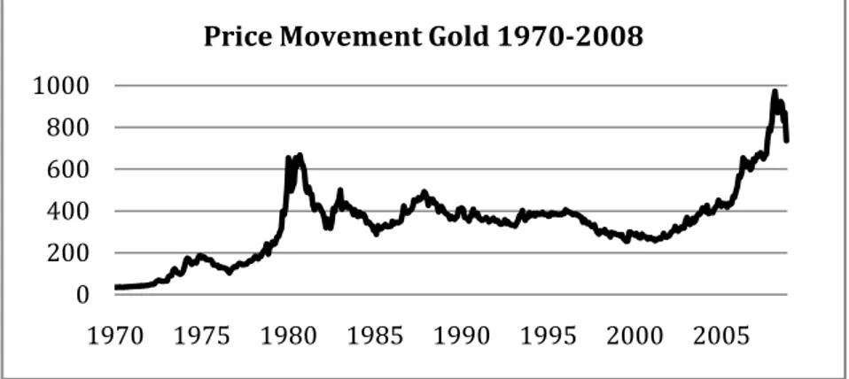
Later in October 2008, Feldman (2008) continued to argue that in today’s insecure financial crisis, investors are still looking for safer forms of investments and that the gold rush is more intense than ever even though the gold prices have reached its peak and is slowly going down again. The reason being that the dollar has become more expensive and the oil prices are plummeting (cited in BBC News, 2008). In addition, the chief analyst Nicholas Brooks at ETF Securities in London is also promoting gold as a safer investment, though it should not be considered a risk-free investment because of its great fluctuations in price (Figure 5) (Dagens Industri, 2008).

Figure 5 Price movement of gold 1970 - 2008

Is gold then the safe have that many believe it to be? In this academic paper, this issue will be looked into more deeply by linking these three main areas of studies: Business Cycles, theo-ries regarding Supply and Demand for Gold, and the Modern Portfolio Theory.

The concept of Business Cycles explains how the economy moves over time with more or less regular fluctuations. It is a part of macroeconomics that explains how the different components of GDP are affecting the market, and how the components themselves are af-fected by peaks and troughs in an economy (Ralf, 2000).

Supply and Demand for gold is the principle mechanism that guides the price of gold, thus the value of gold. Since gold only falls back on its intrinsic value, it receives no interest or dividend payment, the price increase or decrease is what regulates the capital gain. (Le-vin & Wright 2006) The major determinants for gold prices are uncertainty, inflation, gov-ernment auction policy and the supply and demand flow. (Abken, 1980)

Modern Portfolio Theory is based upon theories first introduced by Harry Markowitz, an American economist who was rewarded Nobel Prize in Economics 1990. One of the most important ideas introduced by Markowitz is the use of standard deviation and variance to measure risk. Markowitz also introduced the theory of optimal portfolio selection based on the assumption that investors are risk averse and wants to take as little risk as possible for a given rate of return (Horasanli & Neslihan, 2007).

With these three concepts, this study will aim to investigate if gold can be profitable during recessions when included in an index portfolio.

2.2 Problem discussion

One of the main reasons why this topic was chosen is because a new recession (2008) is threatening many countries all over the world. This makes diversifying investments an im-portant measure to take for private investors. In order to understand these kinds of in-vestments during recessions, one must comprehend the historical economic development

0 200 400 600 800 1000 1970 1975 1980 1985 1990 1995 2000 2005

10

of the market. The US is of special interest because it has influenced the world economy and politics historically, and still today, it is the driving market that influences the global markets.

A returning topic within the fields of safer investments is gold, especially during uncertain times. Historically, gold has been considered a safe haven when other assets have plum-meted due to the unstable situation in an economy. It is therefore of interest to look deeper into this comprehension of gold and its characteristics. Is it possible to look at the histori-cal price movements of gold during recessions to draw the conclusion that an inclusion of gold in a portfolio in today’s recession is profitable? In order to answer this question, nu-merous statistical measures must be taken.

Next step in this process was to find a measure that has represented the movement of the market historically, and is still used today. The Dow Jones Industrial Average (later referred to as DJIA) is one of the most established and renowned indices in the world, and the fact that the world economy is dependent on the US economy makes DJIA an attractive index to look at. By comparing the movement of DJIA, representing the market movement, to gold and its movement, it will be possible to find out whether gold has been the safe haven many proclaim it to be.

However, only having the knowledge about the correlated movement between gold and DJIA is insufficient for a private investor. It is in part helpful for an investor to know about the correlation, but without knowing the optimal allocation of gold, it is rather irrele-vant. Therefore, it is critical to find the optimal portfolio where return to risk is maximized, or to find a minimum variance portfolio for a risk averse investor, where the risk is mini-mized. This will be found by using Markowitz’s portfolio theory and the formulas and equ-ations that are frequently used by the general crowd.

Further research within this field led the research to focus on to what extent gold is per-forming against DJIA from these three perspectives; first, the relative return and risk along with correlation between the two variables in recent recessions. Secondly, the allocation of the two assets an investor should hold and thirdly, if there are significant differences be-tween the allocations for the different recessions.

From this discussion, the final research questions were developed, and these are presented in the subsequent section.

2.2.1 Research questions

The above reasoning led us to the following research questions:

1) Is it possible to conclude whether gold should be invested in when holding a DJIA index portfolio, in order to minimize risk or maximize return given risk, during recessions by looking at past performance of gold and DJIA during the last five recessions in the US? 2) If an investor who possesses a DJIA index portfolio chose to invest in gold during a re-cession, what should the allocation between DJIA and gold be in order to maximize return to risk and minimize risk?

3) Are there any significant differences between the weights and do they vary in different recessions?

11

2.3 Purpose

The purpose of this thesis is to look back at the historical price development of gold and DJIA during recessions in order to find out whether an inclusion of gold can improve a DJIA index portfolio held in today’s recession. In addition, by analyzing the risks and pos-sibilities with gold, the optimal allocation of gold in a DJIA portfolio will be investigated in.

2.4 Approach

The three areas of interest in this paper are the last recessions in the US, gold as an invest-ment, and also the movement of DJIA. Since the study deals with how all these are inter-connected, it is utterly important to get a deep understanding of these topics. Therefore the work of this study will start with investigating the background of all these topics. Thereaf-ter, the Frame of Reference will be dealt with. We have chosen three concepts and theories that we will base our analysis upon. The recessions are explained by the concepts of busi-ness cycles. Gold as an investment will be investigated through the mechanism of supply and demand of the asset, and lastly, in order to tie all of these together we need a portfolio theory. This is because we are interested in not only whether gold can improve the perfor-mance of a portfolio in recessions, but also additionally how one should optimize the port-folio with optimal asset allocation. Therefore we are using the Modern Portport-folio Theory in investigating how much an investor should allocate in gold and DJIA, in order to optimize the holdings. Even though DJIA has few flaws (presented later in a separate section), it is the most widely used index and also an excellent indicator of how the market is moving. In the Result/Analysis, each recession will be analyzed with support from all the informa-tion about the three areas. The empirical findings and analysis for each part will be waved in together to give a more comprehendible view of the situation. Because the main focus of this paper is to investigate in whether gold can be used to increase the return to risk ratio or minimize the risk, it is relevant to compare the results of gold and DJIA with other commodities. This is not included as one of the research questions, however, this will give a more fair view of gold and its relative advantages (and disadvantages) compared to other commodities that are usually used as market indicators. Silver, oil and a commodity index (CCI) have been chosen to compare the gold data to. This will be presented at the end of the Results/Analysis and is mainly included in order to give an investor a well-reasoned in-vestment recommendation. Then, a conclusive analysis will be made where the findings from the data collection and the analysis will be submitted.

12

3 Frame of Reference

In this section, the related economical and financial concepts and theories will be presented. The main parts concern Business Cycles, Supply and Demand for Gold, and the Modern Portfolio Theory. In addition some other important definitions and equations will be introduced.

3.1 Economical theories and concepts

The concepts of business cycles explain how the economy moves over time with more or less regular fluctuations. Business cycles are a part of macroeconomics that explains how the different components of GDP are affecting the market, and how the components themselves are affected by peaks and troughs in an economy. These fluctuations are not af-fected by seasonal changes or single identifiable events, but are spread over longer time span and follow a systematic regular pattern. (Ralf, 2000)

The standard definition of a business cycle is presented by Burns and Mitchell (1946, p.56): “Business cycles are a type of fluctuation found in the aggregate activity of

na-tions that organize their work mainly in business enterprises: a cycle consists of expansions occurring at about the same time in many economic activities, fol-lowed by similarly general recessions, contractions and revivals which merge in-to the expansion phase of the next cycle; this sequence of changes is recurrent but not periodic; in duration business cycles vary from more than one year to ten or twelve years; they are not divisible into shorter cycles of similar charac-ter with amplitudes approximating their own.”

There are several kinds of business cycle theories trying to explain the occurrence of reces-sions and the ‘natural’ fluctuations. The truth of the matter is that recesreces-sions appear for many different reasons; intentionally (e.g. as a direct effect of Fed’s actions) and uninten-tionally (e.g. by natural disasters or terrorist attacks), expected and unexpected. However, until this point no theory has been able to fully explain, without undermining assumptions, why an economy suffers from an economic downturn. The different business cycle theo-ries give varying approaches to the problem from various points of views. These theotheo-ries will not be presented in this study, however, Knoop (2004) has stated six general traits on business cycles in general.

i) Business cycles are not cyclical – looking back historically, the cycles have been any-thing else than cyclical. They have been unpredictable and irregular in both length and duration. The shortest recession in US history was in 1980 with only 6 months’ contraction, while the longest lasted 43 months between 1933 and 1937. In same fashion, the expansions in the economy have varied with the shortest expansion of 12 months to the longest of 121 months. With other words, the length or the depth and severity of a recession or expansion have in no ways given clues on how the next period would look like.

ii) Business cycles are not symmetrical – in the US, a recession have lasted on average 14 months, while an expansion have lasted on average 43 months, more than three times the length of a recession. This clearly shows the asymmetry between ex-pansions and recession, and this asymmetry seems to be true internationally as well. Recessions tend to affect the industrial output more than expansion, and

13

in general, there are shorter but sharper changes in GDP during a recession and a more gradual and slow changes during an expansion.

iii) Business cycles have not changed dramatically over time – Experts often compare the economy by looking at the prewar period and postwar period. Up until ten years ago, economists believed that the postwar business cycles were shorter, less severe, and less frequent. However, with new data presented today, US economists instead mean that there only have been few moderations in the business cycles and the differences between prewar and postwar periods are smaller than earlier believed.

iv) The Great Depression and the World War II expansion dominate all other recessions and expansions – Between 1929 and 1932, GDP fell by 50 % while unemployment rose to 25 % in 1933. To understand the sereneness of the Great Depression, a comparison with the second largest recession in 1973 – 1975 can be made, with a GDP reduction of 4.2 % and unemployment level of 9 %. In the same way, the expansion that started in 1938 continued during the World War II and be-tween 1941 and 1944, GDP increased with 64 %. This is obviously a result of intense mobility of resources and massive government purchases that took place during the war. No other expansions have even come close to the figures during this period.

v) The components of GDP exhibit much different behaviors than GDP itself – GDP is a measure of following components: consumption, investments, net exports, and government spending. Durable consumption (e.g. appliances and automobiles) and investments are both more volatile than nondurable consumption (e.g. food and clothing), government purchases and net exports. Durable consump-tion and investments changes more than output over the business cycle in total (Figure 6).

Figure 6 Behavior of the components of GDP

Figure 6 shows the difference in how each of the components are affected by a fall in GDP, and also how much each component constitute in GDP. Nondu-rables and services both constitute a larger average proportion in GDP, than the average share of contribution when GDP is falling. This means that they are relatively more stable than the GDP as a whole, and are only mildly procyclical. Durables on the other hand are much more volatile than the GDP as a whole,

14

strongly pro cyclical, and a decline in durables can be used as an immediate in-dicator of peaks and troughs in GDP.

Investments are heavily pro cyclical and more volatile than GDP in total. In a recession, the investments are responsible for 70 % of the changes. Govern-ment purchases have 20.6 % of the shares in GDP, but during a recession, the purchases are relatively acyclical meaning that they are only slightly affected by the downturn.

Finally, the net export is a negative balance because the US has had a trade def-icit since mid 1980s. This component is therefore not a reliable indicator of peaks and troughs.

vi) Business cycles are associated with big changes in the labor market – Unemployment is a strongly countercyclical variable (moving in opposite direction) that changes significantly during a recession relatively to any other inputs for production. During recessions and expansions, unemployment counts for two thirds of the changes in GDP per capita, while production counts for remaining a third in GDP per capita. (Knoop, 2004)

3.1.2 Gold

Due to more stable economies the last 20 years, and together with the financial markets’ "invention" of different hedging substitutes, the interest of gold as an investment has de-creased. Due to this, the academic community has more or less ignored researching the possibility of gold as a diversifier. Even though mainstream economists no longer pay much attention to gold, a study conducted by Jonathan Phair (2004) showed that gold still has "great potential for investors".

The main difference between trading with gold and with regular financial assets such as stocks or bonds is that gold is traded from a "store-of-value" point of view, while financial assets are traded in order to secure future income. Consequently, the only gain you will have when investing in gold would be a possible future price increase since it does not yield a return except capital gain (Abken 1980).

As seen in Figure 7, the major supply side factors are recycled gold, mine production and central bank selling, while the demand side constitutes of jewelry, investment and industry demand. Price is the most important aspect considering supply and demand of gold, thus understanding the mechanism of price change will help to understand what drives supply and demand (Solt& Swanson, 1981).

15 Figure 7 Demand and Supply of Gold (World Gold Council)

A more summarized analysis on the determinants of the price of gold was conducted by Abken (1980, p 6), where he located what he called the "probable causes of gold price movements" as: (i) extreme political and economic uncertainty, (ii) flow supply and demand for gold, (iii) inflation, and (iv) government auction policy.

i) Extreme political and economic uncertainty: Since gold throughout history has had rather unique properties such as scarcity, divisibility, uniformity, liquidity, highly mobile, and almost indestructible. Therefore, it has for long time been highly demanded and together with the fact that the increasing above ground stock level (gold that has been extracted and is on the market) grows very slow (due to requirement in in-fra-structure, labor, and capital), gold has always been considered a relatively good store of wealth. This makes gold even more desirable in times of high uncertainty, compared to other assets, as people tend to flee to gold to secure their wealth. ii) Flow of supply and demand for gold: The demand for gold is on one hand the demand of

the goods that was produced using gold in industrial production and also of the gold itself i.e. jewelry. While the supply of gold consists of gold ready for market consumption (above ground stocks). An important notice needs to be made, Abken (1980p 7) states that: “The salient characteristic of gold markets is that changes in flows, i.e., changes in the rate of commercial demand for gold or in gold’s rate of production, affect the stock of gold insignificantly compared to changes in rates of production and consumption on the stocks of other storable commodities. For this reason flow supply and demand for gold have a relatively small impact on the price of gold.” (This section will be treated in depth in section 4.1.2.1 and 4.1.2.2)

iii) The price of gold in terms of dollars is a measurement of the demand of both gold and dollars, relatively. This depends on the believed future rate of return. If the dollar experiences increased inflation, meaning lower dollar value, the relative price of gold should increase by the same amount. For example would a five-percentage in-crease in inflation rate equal a five-percentage appreciation in gold price. As can be seen in Figure 8, the movement of inflation and gold are following a similar pattern.

16

Figure 8 Movement of Price of Gold and US Inflation 1972 - 2004

iv) Government auction policy: Central banks policies of buying and selling gold for their reserves has a big influence on the gold price. Central banks trade gold on special auctions and the market adjusts the price in relation to the announcement of these auctions. So the date of importance is the announcement day and not the exchange day. If a large quantity were sold out, the price would drop and vice versa. Figure 9 displays major world gold holdings 2006.

Figure 9 World Gold Holdings 2006

Now two sections of supply and demand of gold will be presented that elaborates on Ab-ken’s (1980) part ii), because this is of a more complex nature to understand, and has more variables. However, please note that the most significant impacts of gold price movements presented by Abken (1980) are: uncertainty, inflation and government auction policy.

3.1.2.1 Flow supply of gold

Levin & Wright (2006) stated that the short run supply and demand determinants of the price of gold are harder to predict and calculate than the long run since it contains more variables. They assume in their study that the short run price is determined by supply and demand, while long run price is expected to rise in line with inflation. This is because the long run price of gold is linked to the marginal (additional) extraction cost, and if this cost rises in the same pace as inflation, the price will rise in the same rate (this will be furthered discussed in 4.1.2.3).

17

The short run supply of gold has three main sources: mine production (or gold extraction), official sector sales, and recycled gold. Extraction constitutes about 70 % of the supply, but bear no relation to US or global GDP growth (Dempster 2008), figure 10 shows the total mine production in the world since 1980.

Figure 10 Total world mine production 1980 to 2004 Source: GFMS, Ltd.

What then drives the flow supply of gold?

Firstly, Levin & Wright (2006) concluded that the short run supply of gold mining depends positively on price of gold from earlier time periods since the mining industry experience a strong time lag. The price is negatively correlated to the amount of extracted gold that is used to pay off central banks, for the gold leased in earlier periods, and increased by an in-terest rate put on the repayment.

Miners lease gold in the first place in order to supply the market on short notice, in case gold demand rises sharply. In equilibrium the lease rate of gold from central banks equals the convenience yield plus the default risk (convenience yield is the benefit of holding gold in storage for safety). Thus, a fall in interest rate, rise in default risk or rise in convenience yield would reduce quantity of gold leased to the miners from the central banks. The pre-vious period of quantity repaid to prepre-vious rate leased also plays a role on the price of gold, and this is affected by convenience yield and default risk of that same period.

Summing up the short run supply factors of gold from the mining production is current gold price, current and lagged values of physical interest rate, convenience yield and default risk premium. (Levin & Wright 2006)

Secondly, central bank policies to sell out gold are long term strategic and not heavily af-fected by economic cycle tendencies. Through various regulations the central banks have limitations both in size and time in their actions to sell of gold. There exist a time lag be-tween decision, proposition, and actual sale (Dempster, 2008).

Lastly, the recycled gold is determined by many factors and is also heavily volatile in nature (Dempster, 2008). This part is hard to analyze and contributes to the notion made by Levin & Wright (2006), that short run supply is harder to predict than long run.

18

3.1.2.2 Demand of gold

The short-term demand is a function of the "usage demand" (i.e. jewelry, electrical compo-nents etc) and "asset demand" (i.e. dollar expectations, inflation expectations etc) (Levin & Wright 2006).

Dempster (2008, p.6) states, “Conventional wisdom argues that recessions are bad for commodity prices”. Since consumer and business confidence falls, demand on goods falls, meaning that inputs in production decreases. Since many of these goods are commodities, the price of commodities falls. However, Dempster also notes that gold has some impor-tant characteristics that may turn conventional wisdom around. Gold demand for industry is relatively small, thus not relatively vulnerable to business cycles, while gold in electronics is expected to decrease during a recession, since fewer spends less on excess products. Gold in jewelry sector is also more vulnerable than industry demand, but in relation to oth-er precious metals used in jewelries it stands far better in a recession.

The demand in total is based on many other factors, micro economic and macro economic factors, such as, dollar exchange rate factors, inflationary expectations, uncertainty in the economy and political turmoil, returns of other assets, and lack of correlation with other assets. Levin & Wright (2006) In addition to this Gotthelm (2005) argues that gold demand is subject to much uncertainty with the war on terror, the possibility that governments’ re-turn to gold as reserve backing the currencies, dump reserves, or illegalize trade with gold as in the 1930s.

3.1.2.3 Long Run

The long run supply and demand function presented by Levin & Wright (2006) is a func-tion of inflafunc-tion as menfunc-tioned earlier, thus making a good inflafunc-tion hedge. Another impor-tant notification made by Levin and Wright (2006, p.23-24) is “surrounding the assertion that gold reduces portfolio volatility because the types of events that cause stock prices to collapse also tend to raise the price of gold. There is, however a disagreement about the claim that gold has a “negative correlation” because returns to holding gold have the oppo-site sign to the returns on a market portfolio”.

Thus, as seen the factors constituting the price of gold, are highly various in both impact and variability, making gold behave differently from many assets. Some factors are com-mon for others, like inflation, while others, like extraction costs, are solely affecting the gold price.

3.2 Financial theories

3.2.1 Uncertainty and Herd Behavior

In times of financial turmoil where uncertainty about the market increases, people tend to make more irrational decisions. It is reasonable to assume that investors are more willing to invest in safer forms of investments in fear of losing more money. The theory of herd be-havior, derived from the field of psychology, explains how the human kind tends to be more attracted to the behavior of a group rather than an individual act. (Schiller, 1995) In the financial area, investors put a lot of trust on analysts that are believed to have better knowledge than the average investor. Recommendations made by analysts that have had accurate forecasts are given more trust, and in future decisions, the chance that investors will follow that specific analyst’s decision is more likely. In The General Theory of em-ployment, interest and money, written by Keynes (1936), he expresses his concern for

inef-19

ficiency on the market because of the influences of group psychology. Herd behavior un-dermines the information efficiency because the market is no longer driven purely by the in-formation given. Analysts are reluctant to make recommendations in accordance with their beliefs and information if it contradicts with the general perception of the market. Instead they choose to give the same recommendation as the rest of the group, the herd. (Scharfstein & Stein, 1988)

In addition, Avery and Zemsky (1998) mean that the market is driven by ‘animal spirits’. They argue that both market participants and financial economist believe that investors are widely affected by imitative behavior. They are no longer investing rationally; instead they take in influences that are more emotionally attachable.

There are researchers that strongly argue that people consider gold as a safe haven, a safe investment when the economic conditions are unstable and unpredictable. This can be ex-plained by the perception of investors that metals, and in particular gold, is a good diver-sifier during uncertainty. When other investments are declining, gold usually goes up. Another reason to hold on to gold is because of its indestructible physical character; it does not corrode by acids like silver. It is also an asset that is easily traded in forms of jewelry or other physical form. (Gold.org, 2008)

Solt and Swanson (1981) conclude, on the contrary to the statements above in, their article that gold should not be seen as a traditional investment tool. Although in their research, gold had been performing "excellent returns over the last decade (read 1970s)"; there is a considerable risk with gold because of the fluctuations of the gold price. The gold has its own characteristics, and influences that affect the market in general does not apply to the development of gold.

3.2.2 Modern Portfolio Theory

In this study the Modern Portfolio Theory introduced by Harry Markowitz will be used in order to fulfill the purpose. This theory is divided into two parts, a Financial statistical section and a Portfolio theory section. The assumptions made in Modern Portfolio Theory are:

- Investors are rational in the sense that they evaluate the desirability of the assets in terms of expected return and risk.

- They are also assumed to prefer a higher level of return to given risk than lower re-turn (Sharpe, 1964).

- Individual investors are price takers and can invest any portion in the risky assets. - The financial market is free of transaction costs and taxes. (Lintner, 1965)

3.2.2.1 Financial Statistical Section

Return is according to the Oxford Dictionary of Finance and Banking (2005) defined as "the income from an investment frequently referred to as a percentage of its cost." This means the return of an asset can be calculated from the value of the end of the period mi-nus the value in the beginning of the period, divided by the value in the beginning of the period (see Equation 1).

Equation 1 The return of an asset

Rt =

V2−V1

20 V1 = Value of stock at beginning of the period

V2 = Value at end of the period

As past performance often is used as a possible indicator for the future, expected return can be calculated by taking the average (mean value) of the historical returns. The mean values are obtained by taking the sum of all different historical returns, and then dividing the result by the number of different returns (see Equation 2).

Equation 2 Mean value of return

R_A =R1+ R2+ R3

3

Rt = Return for period t.

Expected return for a portfolio is then the sum of the weighted averages of the returns for the assets included in the portfolio (see Equation 3) (Markowitz, 1959).

Equation 3 Expected return for a portfolio

∑

∑

A portfolio consisting of 40% in stock A and 60% in stock B with the given returns of 20% for stock A and 10% for stock B yields a portfolio return (rp) of

(0.4*0.2) + (0.6*0.1) = 0.14 or 14%.

The risk measurement is usually referred to as the volatility of an asset and is viewed as the degree an asset’s return tends to vary around its average or expected return. For an individ-ual asset, risk is measured by variance or standard deviation. Variance for an asset is calcu-lated as the sum of the squared deviations between actual and average return divided by the number of observations (see Equation 4) and standard deviation is simply the square root of the variance (see Equation 5) (Markowitz, 1952). The variance statistic is just the tool used to get to standard deviation, which will be the de facto number. If one calculates the standard deviation from the data set immediately, one would end up with zero fluctuation, due to the cancelling out mechanism between values larger and smaller than the mean val-ue. The variance squares all numbers in order to get the absolute values.

Equation 4 Variance for an individual asset

σ2= (r_t− R)2 t=1 n

∑

rt= return for the specific time period (e.g. weekly, monthly, yearly) R= average return for the entire period

21

n= nr of observations, if a sample is used n should be replaced by n-1. In finance n usually is the nr of time period measured, e.g. n=5 if the analysis covers 5 weeks.

σ2 _{= the variance}

Equation 5 Standard deviation for an individual asset σ = σ2

Example:

A portfolio consisting of an asset that has an average return of 10%, shows during three periods, respective returns of 7%, 11%, and 15%. The variance of the asset would be: ((7-10)2 _{+ (11-10)}2 _{+ (15-10)}2_{)/3= (9 + 1 + 25)/3 = 11.67.}

The standard deviation is correspondingly: √11.67 = 3.42. If one has multiple assets, the variances or standard deviations are summed up.

To compare two assets with different variances (risks), two different statistics called cova-riance and correlation coefficient can be used. The covacova-riance tells you weather two assets' prices move in the same direction or not (see Equation 6). The overall risk for a portfolio can be decreased if assets with negative covariances are included, as the returns will offset each other. Correlation between assets can be calculated in many ways, in this thesis Pearson product-moment correlation coefficient will be used as it is one of the most widely used correlation measures. A correlation coefficient (see Equation 7) scales the covariance between -1 and +1 and tells you in what degree two assets are related to each other. The assets’ returns are more connected the closer the correlation is to -1 or +1. A correlation of +1 means the exact same percentage price movement can be expected for the two assets. A correlation of -1 means exact opposite price movements of the same percentage can be expected. A corre-lation of 0 means the percentage price movements for the two assets are not related at all and are moving without any relation to each other.

Equation 6 Covariance between two returns; RA and RB

Cov(R_A,R_B)= (R_{A ,t} − R _A)(R_{B ,t} − R _B) t=1 n

∑

R _A = mean return for asset A

Equation 7 Correlation coefficient between two assets

ρ_A,B =COV (RA,RB)

σ_A.σ_B

COV(RA,RB)= Covariance between asset A and B. s=variance for the individual assets

The risk for a portfolio of assets is measured by the portfolio variance (as mentioned earli-er) (Markowitz, 1959).

22

3.2.2.2 Portfolio Theory Section

When constructing a portfolio the investment decision process can be conducted in a top-down process. The first implication of the investment decision should be the capital alloca-tion, between risk-free and risky assets. Secondly, the asset allocation should be made, de-ciding the relative quantities between the different risky asset classes, the area in which this study will be conducted. Last, one should conduct security selection, thus deciding between the different securities within each asset class. (Bodie, Kane and Marcus, 2008)

Firstly, the portfolio variance (see Equation 8) can be found by combining all the variances of the individual assets in the portfolio with all the covariances between the very same as-sets weighted by their market weights. The portfolio variance can be lowered if asas-sets not perfectly correlated to any other assets in the portfolio are added to the portfolio (Marko-witz, 1959).

Equation 8 Variance of a portfolio

VAR( p)= w_i2σ_i2+ w_iw_jCOV (R_A,R_B) j=1 n

∑

∑

∑

w= asset weight in the portfolio s2=variance for the individual asset

COV(RA,RB)= Covariance between asset A and B.

When having two risky assets (i.e. gold and DJIA), experimenting with the weights of the assets produces different expected returns and risk combinations to each corresponding weight. All combinations of portfolios that can be created from a set of assets are usually referred to as the opportunity set (see Figure 11). Each dot inside the opportunity set is a possible set of portfolios, and the point at the far left in the middle represents the Mini-mum Variance Portfolio, where the standard deviation is the lowest. The number of port-folios that can be created depends on the correlation coefficient between the assets in the portfolio; the more positive the correlation between the assets is, the less portfolio combi-nations can be utilized. (Sharpe, 1964) (see Figure 12).

Figure 11 Opportunity set of a portfolio

Even though combining different weights of assets can create a big number of possible portfolios, most of them will likely be inefficient, located on the "inside" of the opportunity set. "If a portfolio is inefficient, there is either some other portfolio with more average re-turn and no more standard deviation, or else some portfolio with less standard deviation and no less average return. In the case of most inefficient portfolios there are portfolios which have both more average return and less standard deviation." (Markowitz, 1959).

23

The graph below shows possible combinations of two assets (assets A and B) with differ-ent correlation (the vertical axis describes return and the horizontal axis the risk). As can be seen, when having a correlation value of +1, there is a straight line between A and B. As the correlation decreases, this line concaves to the left indicating a lower risk for the same return.

Figure 12 Return to risk ratio with different correlations

Investors should according to Markowitz (1959) E-V (Expected return – Variance) theory, only construct portfolios where assets are weighted in a way that either gives maximum re-turn for a given level of risk or minimum risk for a given level of return. These portfolios are called efficient portfolios and form a curve called the efficient frontier (see Figure 12) when plot-ted in a graph. When a portfolio is locaplot-ted on the curve, it is called efficient. "If a portfolio is "efficient", it is impossible to obtain a greater average return without incurring greater standard deviation; it is impossible to obtain smaller standard deviation without giving up return on the average." (Markowitz, 1959, p. 22).

To the left of the efficient frontier return-risk levels are unattainable with the current asset allocations, if one does not include risk-free rate (Markowitz, 1952).

Two portfolios that always can be found on the efficient frontier and ease the search for other efficient portfolios are the minimum variance portfolio and the optimal risky portfo-lio. The minimum variance portfolio (see Equation 9) is the portfolio with the lowest risk (variance) on the efficient frontier and the optimal portfolio (see Equation 10) is the port-folio with the highest return to risk ratio on an efficient frontier. These portport-folios can be found both mathematically and graphically.

The weights for the minimum variance portfolio for a portfolio consisting of two risky as-sets can be found by this formula:

Equation 9 Weights for the minimum variance portfolio (MVP)

W_A = σB 2 _{− Cov(A,B)} σA 2 +σ B 2 − 2Cov(A,B) WB = 1- WA

The weights for the optimal portfolio for two risky assets can be found by this formula: Equation 10 Weights for the optimal portfolio (OP)

W_A = [E (RA)− Rf ]σe 2_−[E(R B − Rf ]Cov(RA,RB) [E (RA)− Rf ]σe 2+ [E(R B)− Rf ]σd 2 −[E(R A)− Rf + E(RB)− Rf ]Cov(RA,RB)

24 WB = 1- WA

In order to find the optimal portfolio graphically the Capital Market Line (CML) first has to be found. The CML is the line that gives the relationship between risk and return, in-cluding the risk-free rate. To find the CML, a portfolio must first be constructed, based on the assumptions that investors invest a certain amount in a risk free asset (x) and the rest in the market portfolio e.g. DJIA (1-x).

The return for the constructed portfolio (see Equation 11) can be calculated by this formu-la:

Equation 11 Return for the constructed portfolio R_p = (1− x)R_m+ xR_f

The variance for the portfolio (see Equation 12) can be calculated by this formula: Equation 12 Variance for the constructed portfolio

σp

2 = (1− x)2σ m 2 + x2

0+ 2x(1− x).0

What is left of the portfolio variance (see Equation 13) is the squared weight of the market portfolio times the market portfolio variance.

Equation 13 Variance for the constructed portfolio σp

2 = (1− x)2σ m 2

The standard deviation can be found by this formula: Equation 14 Standard deviation for the constructed portfolio σp = (1− x) σm

After the portfolio is created, the CML can be found by combining the variance and return for the constructed portfolio. The intercept for the line will then be the risk free rate, and the slope is referred to as the market's reward to variability ratio. This ratio tells you, which re-turn you can expect for a certain risk and vice versa for the market portfolio, (see Equation 15) (Sharpe, 1964). As the two assets’ weights must sum up to 1, the CML must be a straight line. If one include a risk-free asset, one get a superior return to risk ratio of this combination to all efficient portfolios, since the risk-free rate has return for zero risk. Equation 15 Capital market line

E(rp)= Rf + (

E(rm)− Rf

σm

)σp

The intercept for the line is Rf (the risk free rate), the slope for the line is: Equation 16 Slope of capital market line

E(r_m)− R_f

σm

The portfolio with the highest return to risk ratio (Sharpe ratio) on an efficient frontier, as mentioned earlier, is the optimal risky portfolio. The mathematical approach has already been discussed. The optimal portfolio can be found graphically at the tangency point of the

25

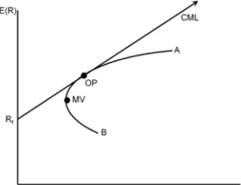
efficient frontier with the CML. When doing that, the CML will meet the efficient frontier at one point and that point is where the optimal portfolio (OP) can be found see Figure 13, (Sharpe, 1964).

Figure 13 Efficient frontier, CML and the location of optimal portfolio

This graph shows the efficient frontier for a combination of the two risky assets A and B. The point A shows the expected return and risk when putting all money in A, and B shows the expected return and risk when putting all money in B. MVP shows the minimum va-riance portfolio, i.e. the portfolio with the lowest risk for the combinations of the risky as-sets A and B. It will always be located at the furthest left point at the efficient frontier. OP shows the optimal risky portfolio i.e. the portfolio that tangents the CML and has the high-est return to risk ratio (Bodie, Kane, Marcus, 2008).

26

4 Historical Background

As this study is based on historical data, it is important to have knowledge about the related history. This part will present the reader with a brief introduction to DJIA and gold. After that, DJIA and gold devel-opment during each recession will be treated, together with graphical illustrations. Recession 2 and 3 are put together due to the close connection in time and possible shared causes and effects.

4.1 Dow Jones Industrial Average

The Dow Jones Industrial Average (DJIA), originally named Dow, Jones & Company, was established in 1882 by Charles Dow, Edward Jones and Charles Bergstresser on 15 Wall Street in New York (Dowjones.com, 2008). At first, only nine industrial stocks were in-cluded, but today, it is an index for the 30 largest so-called Mega Cap world-known com-panies such as Proctor & Gamble, Coca Cola Company, and Microsoft (see Appendix). DJIA is a price-weighted index, meaning that the price of the stocks is divided by the amount of stocks regardless of the relative size. This in turn means that the most influential stocks are those with the highest prices, and if an investor wants to compare the returns on stocks, he would need to buy the same amount of stocks with heavily varied prices. This is not optimal and rational way of investing and it is one of the weaknesses with DJIA. Another disadvantage is that the index only contains 30 US based companies, and industri-al firms represent most of them, which leave many of the companies in the information technology industry outside. However, DJIA is the oldest and first index in US and when people are referring to about how ‘the market’ is doing, DJIA is the most commonly used index. (The Motley Fool, 2008)

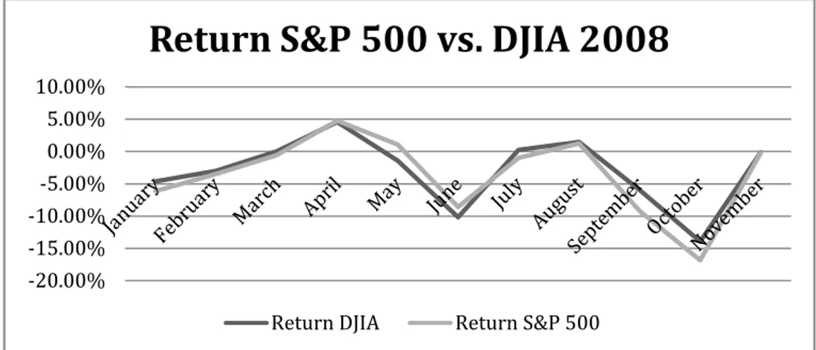
It is not unusual to question the accuracy of DJIA because it is a price weighed index in-stead of a market value weighted index. But when the movement of DJIA was compared to S&P500, which contains 500 companies from Large Cap in the US, the correlation was 0.9487 in the long run and 0.9661 in the short run. (See Figure 14 for short run develop-ment). The high rates indicate the accuracy and are significant, which means that the DJIA is a trustworthy index that reflects the average movement of the stock market just as well as S&P500.

Figure 14 Correlation between S&P500 and DJIA 2008 -20.00% -15.00% -10.00% -5.00% 0.00% 5.00% 10.00%

Return S&P 500 vs. DJIA 2008

27

4.2 Recessions

The National Bureau of Economic Research (later referred to as NBER) is the official or-ganization that announces when a recession starts and ends in the US, and makes other important statistics for the US economy. NBER’s (2008) own definition is:

“The NBER does not define a recession in terms of two consecutive quarters of decline in real GDP. Rather, a recession is a significant decline in economic activity spread across the economy, lasting more than a few months, normally visible in real GDP, real income, employment, industrial production, and wholesale-retail sales. “

The reasons why a recession occurs can differ from time to time. As mentioned earlier, there are several theories, which explain business cycle occurrences from an external and internal point of view. It can start as a reaction to exterior causes such as natural disasters, terrorist attacks or collapse of larger institutions. Internally, the inflation, interest rate and monetary policies can also cause a downturn in the economy. In most cases however, the Fed are trying to protect against an increasing inflation rate, by tightening the money supply, which in turn affects the components of GDP; consumption, investments, net ex-port and government purchases.

4.2.1 Recession 1 1973-11 – 1975-03

The recession that started in 1973 was the second largest downfall in the US economy since the Great Depression in the 30’s. The economy was unstable in the 1970’s, mainly due to the largest corporate collapse in the US history, the Penn Central Railroads that shook the financial markets. The Fed tried to ease the crisis by increasing the money supply, and up to 1973, the effect of the increased liquidity boosted the economic activity. However, even though inflation rose, Nixon (President at the time), was not able to carry out wage and price control and instead he decided to continue supply with money to the economy. (Knoop, 2004)

Another important reason to the high inflation was the abandonment of the Bretton Woods system, where other exchange rates were fixed to the American dollar. In 1971, the US removed the convertibility for gold into dollar, and in 1973 the dollar was floating and enabled even more money growth. The inflation peaked at 5.9 % in 1973 and the real GDP growth was at 5.3 %. However, the main shock to the economy came when OPEC (The Organization of Arab Petroleum Exporting Countries) imposed oil embargo in October same year. The embargo made the oil price rise 300%, from $3 - $12, which in turn started to spin off a chain of negative effects (see Figure 15). Firstly, it reduced real income, which in turn resulted in reduced aggregate demand. Second, and more importantly, it decreased the aggregate supply in two ways; one, it made existing technology and capital stocks too expensive to use; two, it increased the marginal costs for industries where oil was a crucial input. (Knoop, 2004)

In 1975, the inflation turned into stagflation (a status in which the economy experiences both high inflation and unemployment) with a rate that had ran up to 12.1% and unem-ployment had increased from 4.8% to 8.9% from 1973. This recession was the worst since 1930’s and classical economic models on business cycles were discredited, mainly because they could not explain the stagflation phenomenon. In 1975, the oil embargo loosened, and the price of oil and inflation dropped significantly. The economy started to recover with help from the Fed that increased the money supply again. (Knoop, 2004)

28

4.2.1.1 Price movement of Gold Recession 1

The 15th _{of august 1971, president Nixon closed the gold window, suspending all further}

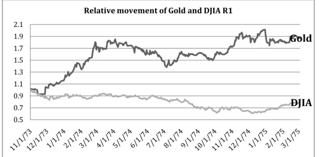
convertibility of USD to gold at 35 USD, in order to strengthen the dollar and stimulate the economy. This had the effect that gold price started to rise, since it was artificially kept at a low rate. As the Soviet Union and South Africa stopped selling gold, decreasing the supply, price soared 14 % in about two weeks. Later the gold price peaked when the Euro-pean Community countries’ stated that they would use a higher rate than earlier decided (38 USD instead of 35 USD), when valuating the official reserves. (World Gold Council, 2008) In 1973, the US trade deficit generated speculation against the dollar, and together with the devaluation of the dollar, and the liberalization of the Japan gold market, the gold price reached all time high of 127 USD.1973 was overall a turbulent year; first, because of the collapse of the Penn Central Railroads and its after affects, secondly, because OPEC halted exports of oil to nations supporting Israel, leading to four time increase of oil price as men-tioned earlier (see Figure 15). This hit the aggregate supply in the US economy. Though, this only generated a marginal change upwards in the gold price at that time. (World Gold Council, 2008)

In the beginning of 1974, gold prices soared as a political turmoil broke out in France. In July the same year monetary policy around the globe was rigid and sale out of gold hoard-ings were done in order to boost liquidity, and therefore the price of gold was lowered to 129 USD from 180 USD (see Figure 15). The oil price increase caused by OPEC, pushed global inflation (with US inflation at 11 %), again increasing demand of gold. (World Gold Council, 2008)

In 1975 US held its first auction of the gold holdings, meaning that citizens were allowed to exchange and own gold and the next year the IMF held its first auction. Now this auction was not well received in the face of stagflation, as mentioned earlier, since people had less money to spend. (World Gold Council, 2008)

Figure 15 DJIA and Gold development during Recession 1

Gold

DJIA

29

4.2.2 Recession 2 1980-01 – 1980-07 and Recession 3 1981-07 – 1982-11

The recession of 1980 was the shortest recession in US economic history with only six month of steady downturn. With very little growth in the end of 1979, almost all macro economic data slowed down in the beginning of 1980. The real GNP growth fell 9.9% in-dicating a strong cyclical contraction and a serious recession. The Fed imposed stronger credit restraint that made the private borrowing drop 51% in second quarter of 1980 (see Figure 16), and at the same time, the interest rates peaked at 20 %. In the third quarter, the interest fell abruptly to 7%. Later this year, the Fed loosened the credit control, and the private borrowing increased again, spiraling in decreased consumer prices, and stable inter-est rates together with a positive consumer expectations and attitude (see Figure 16). (Zar-nowitz & Moore, 2008)

Shortly after the recession in 1980, the most severe economic contraction since the Great Depression was taking place in 1981 – 1982. Like earlier in US economic history, the Fed feared accelerating inflation rate, and in order to hinder the increase, the money supply was severely contracted. According to a study made by Romer and Romer (1994) the industrial growth dropped by 4% a year during years of recessions (cited in Knoop, 2004). They ar-gued further that this would not have been the case if the Fed had not worried about the inflation to a great extent. Rudy Dornbusch (1997, p. 171), an MIT economist, took a step further and argued that “None of the U.S. expansions of the past 40 years died in bed of old age; everyone was murdered by the Federal Reserve”.

4.2.2.1 Price movement of Gold Recession 2 – Recession 3

In 1979, the revolution in Iran broke out, leading to heavy US sanctions of the country. In addition the Soviet Union invaded Afghanistan in the end of the year, yielding a strong in-crease in the price of gold, because of the global turmoil (see p. 12). This had a great effect on gold, which respond to the political uncertainty, leading to gold peaks at 850 USD (see Figure 16), an all time high after the Soviet invasion. At this time, jewelry demand de-creased sharply during the recession while the official sector became a net buyer. In March 1980, gold price had dropped 43% in two months (see Figure 16). In May, IMF completed the four-year sales plan, and conducted its fifth auction for 1980. Later the same year, the first Gulf War broke out in September, leading to higher oil price and inflation. (World Gold Council, 2008)

After soaring gold prices in 1979 and 1980, the prices fell almost 200 USD in 1981 (see Figure 17) after record high interest rates, where the Fed Funds rate was 19 % in June 1981 (this in order to hinder the accelerating inflation). Thus, in this recession gold price de-creased as more people put their wealth in interest bearing bills. In addition as the Fed tervened in the market in 1982, the confidence in the American dollar was restored and in-flation decreased, which lowered demand for gold (see Figure 17) (see 4.1.2) (World Gold Council, 2008).

30 Figure 16 DJIA and Gold development during recession 2

Figure 17 DJIA and Gold development during Recession 3

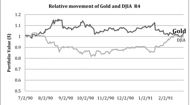
4.2.3 Recession 4 1990-07 – 1991-03

There are several theories on why the recession during this period actually occurred. In July 1990, the US economy had experienced the longest post wartime expansion in the eco-nomic history. The downturn has been explained by shifting consumer preferences, the oil price shock caused by Iraq’s invasion in Kuwait and once again, the Fed’s attempt to hind-er the inflation by monetary policies. The inflation had risen from 1.2% in 1986 to 4.4% in

Gold

DJIA

Relative movement of Gold and DJIA R2

Gold

31

1989. But already in 1986, the Fed had sensed that inflation could be a possible outcome, and in order to reach zero-inflation (which was argued by experts to spur average real eco-nomic growth) they imposed a contraction policy. However, in early 1989, the aggregate spending factors turned down sharply and eventually put the slowly growing economy into recession. (Walsh, 1993)

According to Poole (2007), the 75% oil price increase caused the main downturn in the economy. The oil shock began in August 1990, and in October the same year the inflation was at 6.4%. Hamilton and Herrera (cited in Poole, 2007) meant that there was a correla-tion between increasing oil prices and down turning economies. The price increases in 1973, 1979 and 1990 all led to a recession within a year in the US economy. However, Poole (2007) wanted to point out that even though the oil prices (an external factors) could trigger a recession, it would not be possible to create a recession if the economy already was not over heated (Siegel 2007).

4.2.3.1 Price movement of Gold Recession 4

In first nine months of 1989 gold prices moves downward due to forward sales in Australia and still high interest rates, but gold recovered in the end because of speculative buying at the height of the Tiananmen Square protest in Beijing, adding uncertainty in the global community. The price again moved down shortly after to a three-year low of 355 USD, and changed direction up to 400 USD again after speculative buying. (World Gold Council, 2008)

The gold price started very volatile in the 90’s, first down under mistrust against covert sell-ing from Soviet, and further down in March when a major bank in the Middle East liqui-dated large amount of its holdings (read section 4.1.2 for further information). Although gold price soared shortly when Iraq went into Kuwait in August, the ending rate was as the beginning of the year (see Figure 18). The price increased to 403 USD when the Allies went into Iraq in January 1991, but went quickly down again due to overall global stability before the end of Soviet Union. When the Soviet Union was dissolved, gold investments went down since the political tension was remarkably decreased. (World Gold Council, 2008)

Figure 18 DJIA and Gold development during recession 4

Gold