2005:64 Investigating conceptual models for physical property couplings in solid solution models of cement

SKI Report

2005:64

Research

Investigating conceptual models for physical

property couplings in solid solution models

of cement

Steven Benbow

Claire Watson

David Savage

November 2005

SKI Perspective

Background

Concrete and cement are used in constructions as well as in conditioning of waste in repositories for radioactive waste. The long-term degradation of the cement produces alkaline waters that can influence other barriers, which has been investigated in earlier SKI studies. The degradation process can also change the physical properties of the cement itself and e.g. change the transport properties.

Purpose of the project

The purpose of this project is to develop a more realistic cement model by

implementing a solid solution gel model into a geochemical modelling framework (within the Raiden code). The model will predict the time-dependent evolution of cement pore fluid, with generally decreasing pH over time. The changing physical properties of the cement will then be explored. The buffering capacity of the

surrounding backfill is accounted for by using backfill models earlier developed for SKI.

Results

The modelling shows that it is possible to couple various conceptual models for the evolution of physical properties of concrete with a solid solution model for cement degradation. A fully coupled geochemical transport model to describe the interaction of cement/concrete engineered barriers with groundwater has been used. The modelling also shows results that are sensitive to different variants of the conceptual models for transport properties and for variations in flow rates. For instance more or less pore clogging is noticed. Most simulations were carried out for a reduced ‘experimental’ scale rather than a full repository scale.

Effects on SKI work

The work has shown the possibility to investigate also the changing physical properties of degrading cement. To further develop the model more emphasis is needed on kinetics and the detailed development of a nearly clogged pore space. Modelling of the full repository scale could be another way forward to understand the behaviour of degrading concrete.

A general conclusion is that the combined effects of chemical evolution and physical degradation should be analysed in performance assessments of cementitious

Project information

Responsible for the project at SKI has been Christina Lilja. SKI reference: SKI 2004/182/200409111

Research

Investigating conceptual models for physical

property couplings in solid solution models

of cement

Steven Benbow

Claire Watson

David Savage

Quintesssa Limited

Dalton House

Newtown Road

Henley-on-Thames

Oxfordshire

RG9 1HG

November 2005

SKI Rapport 2005:64

Contents

Summary 1

1 Introduction 5

2 Börjesson et al.’s non-ideal solid solution model for CSH gel 7

2.1 Solid solution computer codes 8

2.2 Implementation in Raiden as kinetic reactions 9

2.3 Model 9

2.4 Raiden model 10

2.5 Results 15

2.6 Conclusions 19

3 Experimental-scale EBS modelling and conceptual models for transport

properties 21

3.1 Mineralogy 23

3.1.1 Initial concrete and backfill compositions 23

3.1.2 Secondary minerals 24

3.1.3 Mineral physical properties 27

3.1.4 Rates of reaction 28

3.2 Fluids 31

3.3 Reference physical properties of the cement and backfill 33

3.4 Coupling cement physical properties to degradation 34

3.4.1 Permeability – the Kozeny-Carmen relation 34

3.4.2 A Kozeny-Carmen relation for composite media 36

3.4.3 Diffusion – Porosity 40

3.4.4 Flow 41

3.5 Summary of variant cases 42

3.6 Implementing degradation-dependent material properties in Raiden 45

4 Simple flow-through modelling results – Identifying a base case 47

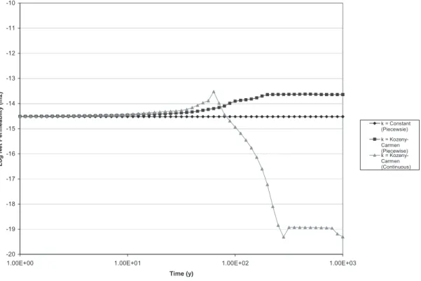
4.1 Varying the permeability model 47

4.1.1 Choosing a base model for permeability for the subsequent modelling 59

4.2 Varying the effective diffusion model 59

4.2.1 Comparing Archie’s law with the constant diffusion model 60

4.2.2 Varying the Archie’s law parameter 62

4.2.3 Choosing a base model for diffusion for the subsequent modelling 65

4.3 Varying flow rates in the base case model for permeability and diffusion 66

5 Simple models with backfill jackets 69

7 Secondary tobermorite cases 85

7.1 The no backfill jacket model 86

7.2 The backfill jacket model 86

8 pH buffering in the experimental-scale models 89

9 Experimental-scale models with fractures 93

9.1 Fracture zone results 94

9.2 Single fracture results 102

10 General observations on the experimental-scale modelling results 105

11 Preliminary site-scale models 109

11.1 Clogging time vs. clogging distance 119

11.2 Degrees of degradation 120

11.3 pH buffering capacity of the backfill 120

11.4 Summary of repository-scale modelling results 121

12 Conclusions 123

Appendix: Input files for the simple box model 127

Summary

The long-term behaviour of cementitious engineered barriers is an important process to consider when modelling the migration of radionuclides from a geological repository for nuclear waste. Many geological disposal concepts incorporate cement either to encapsulate the waste forms, to provide a chemical buffer, or to provide structural integrity for the underground system of deposition tunnels. In the presence of invasive groundwater, the chemical and physical properties of cement, such as its pH buffer capacity, resistance to flow, and its mechanical properties, can evolve with time. A variety of transport, chemical, and mechanical processes play an important role in the degradation of concrete and must be better understood in order to quantify such effects. The modelling of cement is complicated by the fact that the cement is dominated by the behaviour of calcium silicate hydrate (CSH) gel which is a complex solid exhibiting incongruent dissolution behaviour. In this report, we have demonstrated the

implementation of a solid-solution CSH gel model within a geochemical transport modelling framework using the Raiden computer code to investigate cement/concrete-groundwater interactions.

The modelling conducted here shows that it is possible to couple various conceptual models for the evolution of physical properties of concrete with a solid solution model for cement degradation in a fully coupled geochemical transport model to describe the interaction of cement/concrete engineered barriers with groundwater. The results show that changes to the conceptual models and flow rates can give rise to very different evolutions. Most simulations were carried out at a reduced ‘experimental’ scale rather than full repository scale.

Calculational cases with no backfill generally displayed significant cement degradation. Such levels of degradation may not be expected to be typical repository scale

evolutions, since in the model, the flow and transport was constrained to pass through the sample to provide maximal amounts of degradation as might be typical in flow-through experiments. However, these simulations showed that:

• The portlandite inventory was depleted in all cases, but in many cases, a significant amount of CSH remained, following clogging of the upstream and downstream ends of the sample.

• All cases exhibited a significant amount of tobermorite precipitation at the downstream end of the sample.

• For fast flow cases, the degradation of the concrete was well characterised as a function of the total amount of water that had flowed through the sample.

• Changing the physical model led to changes in formation products. For example, using the Archie’s law diffusion model led to tobermorite precipitation at the upstream end of the sample, rather than calcite.

• In slow flow cases, the dependency of the time taken to degrade the concrete by a

specified amount (volume fraction) on the Archie’s law parameter, m appeared to

be close to linear and increased with m.

• Changing the flow velocity affected the amount of degradation, but also affected the solid products – more calcite at the upstream end was observed for faster flows. Hence forced advection would not appear to be a good method of simulating up-scaled time diffusion processes.

• Faster flow rates did not necessarily lead to faster clogging of the cement/concrete. All simulations with a backfill jacket displayed rapid dissolution of the cement phases. Degradation was more rapid than the models with no backfill, since the forced flow through the sample allowed clogging at both ends. This was not the case for the backfill jacket models, where no regions became totally clogged. Large area to volume ratios of the concrete sample caused diffusion-dominated dissolution of the cement. Once the cement was totally dissolved, a fast pathway appeared through the centre of the sample region.

Simulations with two different groundwater compositions were considered, Finnsjön non-saline (a high carbonate water), and Äspö saline (a high sulphate water). However, the choice of groundwater did not significantly affect the lifetime of the concrete, although the Finnsjön water was marginally quicker at dissolving the concrete. The stability of the secondary solid products was different for the two waters. Precipitated tobermorite was rapidly converted to calcite once the cement inventory was depleted with the high carbonate Finnsjön water, whereas the tobermorite formation was more stable with the Äspö water and was only slowly converted to calcite.

In all simulations, tobermorite was greatly oversaturated in the concrete regions of the model, where it was not allowed to precipitate. If tobermorite was allowed to

precipitate within the cement region (as it might during cement ageing), then all of the CSH in the model was converted to tobermorite within the first year of simulation (note that realistic ageing kinetics were not included). Portlandite evolution was largely unaffected; it dissolved slightly quicker in the cases when CSH was present but not significantly quicker. After depletion of portlandite, the tobermorite was converted to calcite, but the timescales for this were longer than for the depletion of CSH in the original models.

The peak pH at the outlet was around 12 for most simulations, and either decreased to host rock pH if the concrete sample was dissolved or stabilised at a pH that was consistent with the clogging minerals in the cases when pore clogging occurred to seal the concrete sample. It should be noted that this high pH was not predictive of a high pH in the repository scale system, where the length scales in the simulation were very

different. However the results are indicative that the peak pH emanating from the concrete was not especially sensitive to the characterisation of the permeability and diffusion coefficient models, but obviously the duration of the high pH will depend on the lifetime of the concrete and/or its eventual clogging.

Some models were run with simulated fractures in the concrete region. In models where the formation of secondary CSH species was disallowed in fractures, the evolution of the system was not dramatically different from the non-fractured cases. When secondary CSH was allowed in the fractures, the difference in evolution was dramatic, with ensuing clogging of the pore space. Degradation of the neighbouring concrete took place until the pore space was clogged completely. If the pore space did not clog entirely, then the sample completely dissolved.

Full repository-scale models showed that in all cases, the pore space adjacent to the concrete became clogged. The time for clogging ranged from 1000 years for the fast flow case to around 3000 years for the slow and no flow cases. At the time of clogging, a significant amount of the cement was still present in the system. Over 80 % of the portlandite was present in all cases, and little to no CSH dissolution was seen. This was in contrast to the experimental-scale models where all variants showed a significant reduction in portlandite and CSH content. The major formation product was

tobermorite, although the amount of calcite increased with the flow speed. Calcite was seen in significant amounts in the fast flow case. The backfill buffered pH to a limited extent, maintaining pH below 10 in the fast flow case, 11 in the slow flow case and 11.5 in the no flow case. The time taken to armour the backfill to a range of depths from 0.5 cm to 25 cm was investigated and it was found that the armouring time was well characterised as a quadratic function of the armouring depth.

There is of course some uncertainty regarding how to continue modelling after pore-clogging takes place. In the case of 1D models, most studies consider pore-pore-clogging to be a halting criterion for the model as no further transport in the model is possible. In 2D models the clogged cells are often switched off to prevent further transport through the clogged area. Both of these approaches lead to regions in the model that cannot experience further evolution. In reality it may be the case that the mechanical couplings cause the precipitated minerals, or the host media, to break up. This will depend on the confinement of the system and the strength of the various minerals. Alternatively it could be the case that the precipitated materials have some inherent conductivity, albeit small, due to their method of formation or structure. In the modelling presented in this report, mineral reactions are limited when porosities become very small (of the order of 10-4). This forces the clogged regions to remain open to trivial amounts of continued transport, and hence allows the clogged region to continue to evolve, and potentially unblock if porewater conditions evolve to eventually undersaturate the precipitated minerals.

the model then secondary precipitation would be slowed and may possibly not lead to total clogging in regions of the system.

The choice of model for the cement kinetics can also give rise to different evolutions of the system. In this study we have adopted a consistent solid-solution model of the cement region, but other formulations are available that could lead to slightly different evolutions and timescales of evolution.

Future modelling of this type could address some of the uncertainties described above, and could also consider:

• A more detailed investigation at full repository scale; • Alternative models for cement behaviour.

1 Introduction

The reaction of cement with groundwater is an important process to consider when modelling the migration of radionuclides from a repository for nuclear waste. Many disposal concepts incorporate a cement region to either encapsulate the waste forms or provide structural integrity for the underground system. In the presence of an invasive host water, the physical properties of the cement, such as its resistance to flow and its mechanical properties, can evolve with time.

As pointed out by Pfingsten (2001), cement and concrete in a waste repository may be degraded by interaction with ambient groundwater because of the large chemical

gradient of species such as OH- and HCO3- across the near-field and surrounding

rock-groundwater system. The potential consequences of these gradients are the progressive

removal of OH- from the cement and the precipitation of calcite which may ‘armour’ the

cement surface, both reducing the effectiveness of the pH buffering capacity of the cement. It is conceivable that, in the long-term, fracturing of the cement mass, coupled

with OH- removal and calcite armouring of cement ‘blocks’ will impact upon the

capacity of the cementitious engineered barriers to buffer pH at elevated values (pH > 12) and act as sorption surfaces for released radionuclides. Clearly, some

coupled description of hydraulic, transport, and chemical processes is required to assess the relevance of these processes to barrier performance and waste isolation.

The modelling of cement is complicated by the fact that the cement is dominated by the behaviour of a complex non-crystalline calcium silicate hydrate phase, which has

incongruent dissolution behaviour. CSH gel does not have a fixed chemical composition but has a variable Ca/Si ratio, from approximately one, to two, or higher. It is a near-amorphous material, but can be considered to have a ‘degenerate clay structure’

(Mindess and Young, 1981), by which is meant that it can be thought to have a layered structure, consisting of sheets of calcium silicate with interlayer calcium ions and water. At solid Ca/Si ratios > 1, CSH gel dissolves incongruently in water with aqueous Ca concentrations being much higher than those of Si. The extent of incongruent dissolution behaviour increases with the Ca/Si ratio of the solid. Ca-rich CSH gel (Ca/Si > 2) equilibrates with aqueous solutions of very high Ca/Si ratio (> 10 000), whereas low Ca/Si gel (Ca/Si ≤ 1) coexists with an aqueous phase with a

Ca/Si ratio < 1. Despite the non-stoichiometric dissolution behaviour, there is good evidence that dissolution behaviour is driven by thermodynamic equilibrium.

A number of different models have been proposed to describe CSH gel behaviour, the

most common of which are those relying upon solubilities in the system CaO-SiO2-H2O

being recalculated to unique solubility products raised to fractional powers as a function of the Ca/Si ratio (e.g. Glasser et al., 1988). Greenberg et al. (Greenberg et al., 1960)

In this report, we first demonstrate the implementation of the cement model of

Börjesson et al. in the Raiden geochemical transport modelling framework (Benbow et al., 2005). The model implemented in Raiden is then compared with published results obtained using the SOLISOL code (Börjesson and Emrén, 1993), which implements the solid solution cement model.

In Section 2 we introduce the solid solution model for CSH gel developed by Börjesson et al. (1997a) and describe its mathematical formulation and the implementation in Raiden. We compare the model generated using Raiden with published results and discuss time-stepping issues that arise from the comparison.

In Section 3 we describe the experimental-scale models that are used to investigate the various couplings between degradation and the physical properties of the cement and discuss conceptual models for implementing the couplings. Dependency of

permeability on degradation is often described by the Kozeny-Carmen relation (see for example, de Marsily, 1986), which expresses permeability as a function of porosity. In Section 3.4 we propose a generalisation of the relationship to model more realistically composite media systems. The same approach is also applied to Archie’s law for the effective diffusion coefficient as a function of porosity.

Results from the experimental scale models are presented in sections 4 to 9. In Section 4, simple 1-D models where flow is forced through a concrete sample are considered. In Section 5, simple 2-D experimental scale models with backfill pathways around a concrete sample are considered and the results are compared with the forced flow simulations. Variations of pore water chemistry are discussed in Section 6 and in Section 7 results are presented using an alternative conceptual model for cement formation products. Since the high pH water produced from the cement degradation and its subsequent buffering is a key performance measure for repository design, pH buffering evolution in the experimental scale models is summarised in Section 8. In Section 9, some of the previous models are rerun with alterations to the geometry to represent the presence of fractures or fracture zones in the concrete sample.

Some key observations from the results presented in sections 4 to 9 are summarised in Section 10.

Finally, in Section 11 some preliminary models that use the core conceptual models developed in the experimental scale models are implemented in a more realistic repository scale geometry.

2 Börjesson et al.’s non-ideal solid solution

model for CSH gel

In this section we describe the approach to modelling CSH gel as a two end member solid solution as proposed by Börjesson et al. (1997a), together with the implementation of the approach in the Raiden coupled geochemical modelling and transport code (Benbow et al., 2005).

In Börjesson et al. (1997a), CSH gel is assumed to consist of two end members,

Portlandite (Ca(OH)2) and a fictive calcium silicate solid (CaH2SiO4), with the

following equilibria:

Table 2.1: Cement end members.

Phase Reaction Log10 K†

Ca(OH)2 Ca(OH)2 + 2H+ = Ca2+ + 2H2O 23.1

CaH2SiO4 CaH2SiO4 + 2H+ = Ca2+ + SiO2(aq) + 2H2O 14.90

We will denote the two end members Ca(OH)2 and CaH2SiO4 by M1 and M2

respectively; and will denote the concentration (mol/m3) of Mi by C . The mole _i

fractions X of each member are then given by _i

2 1 C C C X i i = ₊ .

(Note that the reported concentrations in Raiden correspond to the values C ). _i

Börjesson et al. (1997a) develop a model for the non-ideal solid solution for CSH gel as follows. The excess Gibbs free energy of the cement can be expressed in terms of a power series of the difference in the mole fractions between the two end members:

(

)

(

)

(

)

This is referred to as the Guggenheim thermodynamic mixing model. Börjesson et al. (1997a) consider only the first two terms in the expansion, thus

∑

= _{i i}

excess RT X

G ln

γ

where

γ

in the cement is then taken to be i

i i X

a =

γ

Equating the two expressions for G_excess gives

(

)

[

]

(

)

(

)

[

]

(

)

Hence the activities of the end members are given by

(X X ) RT E e X a , / 1 1 = 1 1 2 (2.1) and (X X ) RT E e X a , / 2 2 = 2 1 2 . (2.2)

2.1 Solid solution computer codes

Börjesson et al. initially developed a computer program, SOLISOL (Börjesson et al., 1993), which is essentially a wrapper for the PHREEQE geochemical modelling package. The original SOLISOL code did not use the Guggenheim thermodynamic mixing model as outlined above, but instead used PHREEQE to calculate equilibrium concentrations given log K values for the cement that are calculated by SOLISOL as a function of the C/S ratio assuming an ideal solid solution.

Börjesson et al. later developed the PASSIPHIC modelling program (Börjesson et al., 1997a) to treat non-ideal solid solutions. The PASSIPHIC code uses a modified version of the SOLISOL code that implements the Guggenheim thermodynamic mixing model described above.

Neither the original nor modified versions of the SOLISOL code can treat transport; they are purely equilibrium models. To treat the evolution of a modelled system, SOLISOL has to repeatedly call PHREEQE to calculate new equilibria given new starting conditions, and has to attach a notional timescale on the time taken to reach equilibrium. This approach is sensible when modelling experimental systems where a leaching solid is exposed to a water that is flushed at regular time intervals (where the time interval is greater than the time required for the solid to equilibrate with the water), but is not so useful for performing continuously evolving geochemical calculations.

2.2 Implementation in Raiden as kinetic reactions

Using Börjesson et al.’s approach, we can easily write a Raiden procedure that

calculates the activities of the cement end members given the concentrations of the solid and aqueous species in the system using the equations in Section 2.

Given the activities of the end members, we can then calculate the saturations of each. If we write: ( )

[ ]

[ ]

[

]

[ ]

[

]

[

]

[ ]

where [.] denotes activity and a_{Ca( )OH2} and a_CaH2SiO4are given by equations (2.1) and

(2.2), we can then write a kinetic reaction for the dissolution/precipitation of each end member. Specifically we can use a Transition State Theory rate equation (e.g. Helgeson et al., 1984) of the form,

⎟⎟ ⎠ ⎞ ⎜⎜ ⎝ ⎛ − = 1 i i i i i K Q A k dt dC .

Here k_i(mol m-2 y-1) is the rate of the reaction per surface area of end member and A_i is

the surface area of the end member per m3. If we want to model the solid-solution as

being essentially instantaneous, we can choose k_i to be large compared to the other

reaction rates and timescales in the system.

2.3 Model

We have compared the model for CSH gel developed in Raiden above with that described by Börjesson and Emrén (1993). Börjesson and Emrén (1993) use the original version of SOLISOL to model the leaching of cement with a synthetic groundwater; the model being comparable to experiments conducted by Lundén and

of 1 week was attached to each equilibration step, thus simulating an experiment where the water in the system was flushed and replaced with fresh water on a weekly basis (and where it is assumed that the time taken to equilibrate the water with the cement, regardless of how much cement is present, is less than 1 week).

Table 2.2: Synthetic groundwater composition.

Element Concentration (mM) Na 1.13 K 7.16 x 10-2 Ca 0.25 Mg 8.80 x 10-2 Al 1.11 x 10-4 Si 0.33 Fe 5.37 x 10-3 Cl 2.21 S 0.11 pH 8.2 pe 5.34

Table 2.3: Cement sample.

Substance Quantity (mmol)

Ca(OH)2 787.6

CaH2SiO4 342.9

KOH 23.26 NaOH 6.46

Reasonable agreement with the experimental results was observed. The KOH and NaOH minerals were included in the modelled system in order to try to match an observed early spike in pH, with both of these minerals completely dissolving in a short

time to introduce extra OH- to the system.

2.4 Raiden model

Since the Raiden conceptual model is of continuous evolution, rather than static equilibration, the model as set up by Börjesson et al. cannot be implemented directly. Instead, a model has been set up in which the ratio of the amounts of flushing water to the amount of cement are similar to those in Börjesson et al.’s model.

The Raiden model simulates the continual advection of the synthetic porewater through a cement sample. The cement sample is taken to have a very large porosity to emulate the large water volume to concrete volume ratio in Börjesson et al.’s model, as shown in Figure 2.1. 1 m2 1 m2 1 m Solid phase Highly porous Flow direction

Figure 2.1: Raiden conceptual model.

Table 2.4: Properties of CSH species.

Substance Molar weight (g/mol) Molar volume (m3/mol)

Ca(OH)2 74.0927 33 x 10-6

CaH2SiO4 134.1767 60 x 10-6†

The molar weights and volumes assumed for the CSH species are shown in Table 2.4. (This leads to a cement sample of ~104.4 g compared to 100 g assumed by Börjesson et

al.). In Raiden it is convenient to model a 1 m3 total volume (1x1x1 m).

The calculations to convert Börjesson et al.’s input data to Raiden input data are as follows.

Denote by Ni the number of mol of each mineral per litre of water in Börjesson et al.’s

model, and denote the porosity of the 1 m3 volume by θ . Then there are

θ

∑

of each mineral per m3. The volume occupied by the minerals is therefore θ

∑

m3, where Mvi denotes the molar volume of mineral i (m3/mol). Thus

1 Mv

N =

+θ

∑

∑

Using the molar volume data presented in Table 2.4, and ignoring the volume occupied by the KOH and NaOH species (which will be small), the porosity required to give the same water to solid ratio as in Börjesson et al.’s model is approximately 0.956.

The resulting initial mineral concentrations are given in Table 2.5.

Table 2.5: Solid composition in Raiden calculations.

Substance Concentration (mol/m3)

Ca(OH)2 752.56

CaH2SiO4 327.65

KOH 22.23 NaOH 6.17

The water in the SOLISOL model is assumed to be replaced once per week, thus an equivalent volumetric flow rate is around 52.2 litres per year (per 100 g of cement).

The volume of water in the Raiden model (initially) is ₁₀3

θ

equivalent flow rate in the Raiden model is _52.2×103

_θ

to replace all of the water in the volume approximately once per week), which is around

50 m3/y. Assuming 1m2 faces on the volume for incoming and outgoing water, we

arrive at a Darcy velocity in the Raiden model of 50 m/y.

It is easiest to attempt to fix the hydraulic conductivity, K, of the volume at 1m/y, then the desired flow rates can be achieved by defining a head difference of 50 m across the

1m flow length of the volume. If acceleration due to gravity, g, is taken to be 10 m s-2,

density of water,

ρ

μ

10-3 Pa s, then the permeability, k, such that the desired hydraulic conductivity of 1 m/y

is obtained is approximately k ₌10-7/S_ym2_{, where}

y

S is the number of seconds per

year.

The thermodynamic properties of the minerals in the model are shown in the

Geochemist’s Workbench (Bethke, 1996) database snippet in Figure 2.2. Note that the

log K values for Ca(OH)2 and CaH2SiO4 have been converted with respect to basis

species H+ and SiO2(aq) (Börjesson et al. used OH- and H2SiO42-). The log K values for

KOH and NaOH have been arbitrarily chosen to be large enough to force complete dissolution of these phases during the early simulation.

The pe of the synthetic groundwater in Börjesson et al.’s model has been converted to

It is not clear which secondary aqueous complex species were included in Börjesson et al.’s model (no input file is available to rerun Börjesson et al.’s case). The species chosen in the Raiden model are listed in Table 2.6.

Input files for the Raiden model are listed in the appendix.

Portlandite type= formula= Ca(OH)2

mole vol.= 33.056 cc mole wt.= 74.0927 g 3 species in reaction -2.0000 H+ 1.0000 Ca++ 2.0000 H2O 24.6242 23.1 20.1960 18.0608 15.9702 14.3128 12.9403 11.7465 ... CalciumSilicate type= formula= CaH2SiO4

mole vol.= 60.000 cc mole wt.= 134.1769 g 4 species in reaction -2.0000 H+ 1.0000 Ca++ 1.0000 SiO2(aq) 2.0000 H2O 14.9072 14.9072 14.9072 14.9072 14.9072 14.9072 14.9072 14.9072 ... NaOH type= formula= NaOH

mole vol.= 0.000 cc mole wt.= 135 g 3 species in reaction -1.0000 H+ 1.0000 Na+ 1.0000 H2O 1000.0000 1000.0000 1000.0000 1000.0000 1000.0000 1000.0000 1000.0000 1000.0000 ... KOH type= formula= NaOH

mole vol.= 0.000 cc mole wt.= 135 g 3 species in reaction

-1.0000 H+ 1.0000 K+ 1.0000 H2O 1000.0000 1000.0000 1000.0000 1000.0000

Table 2.6: Initial concentrations of pore water species in the Raiden model.

Species Basis/Complex/Redox Initial

concentration (mol/kg)

HCO3- Basis 1e-012

O2(aq) Basis 1.38393e-032

Al(OH)4- Basis 1.11e-007

Ca2+ Basis 0.000249995 Cl- Basis 0.00221 Fe2+ Basis 5.36969e-006 K+ Basis 7.16e-005 Mg2+ Basis 8.8e-005 Na+ Basis 0.00112971 SO42- Basis 0.00011

SiO2(aq) Basis 0.000323258

H2O Basis 55.5084

H+ Basis 6.26012e-009

Al3+ Aqueous 2.95208e-018

CO32- Aqueous 9.39923e-015

CaOH+ Aqueous 5.0363e-009

NaHSiO3(aq) Aqueous 2.8969e-007

HSiO3- Aqueous 6.45215e-006

H2SiO42- Aqueous 1.27086e-010

Fe(OH)2(aq) Aqueous 3.07289e-010

HCl(aq) Aqueous 2.64081e-012

Al(SO4)2- Aqueous 1.14555e-021

AlSO4+ Aqueous 1.68305e-019

OH- Aqueous 1.80948e-006

HS- Redox 1.38157e-087

2.5 Results

The pH results from Börjesson et al.’s model (using the original version of SOLISOL) and the Raiden model are shown for 10 weeks of simulation in Figure 2.3 and 50 weeks of simulation in Figure 2.4. The initial early peak in pH is due to the dissolution of the KOH and NaOH solids. From the results over 10 weeks, it can be seen that the

simulated pH in the Raiden model is similar to that predicted by SOLISOL. It would not be expected that the results would match perfectly, since the original version of SOLISOL does not use the Guggenheim thermodynamic mixing model and the full details of the pore water chemistry in the modelling are not known. Given this, the results appear encouraging.

The results to 50 weeks show that, for the first 15 weeks the Raiden and SOLISOL models agree fairly closely, but after that time, the Raiden model begins to approach a new equilibrium more smoothly than the SOLISOL model. The equilibrium that is approached by both models is similar, and Figure 2.5 shows that the trigger for the new equilibrium is the total depletion of the Portlandite in the cement. The difference in the approach to equilibrium in the two models is most likely due to the different

timestepping approaches taken in the two models. The Raiden approach uses an adaptive time-stepping approach, whereas the SOLISOL model simply equilibrates the pore water with respect the solid phase and attaches a notional timescale of one week for equilibration, after which time the pore water is replaced and the calculation

repeated. It would seem natural that the actual time for equilibration with respect to the pore water would depend on the amount of the solid phase that is present in the system, and that the equilibration time would increase as the amount of solid decreases. Thus at early times in the SOLISOL model it may be that the assumed timescale of 1 week is too long, whereas at later times it may be too short. Perturbing the timescales in the SOLISOL model to account for this inconsistency in timescales would lead to a curve that looked qualitatively more similar to the Raiden curve. The graph does however show that after one year, given the same volumetric flow rates of water in both models, the overall change in pH is similar.

Figure 2.6 shows the continuation of the Raiden simulation to 10 years; from which it can be seen that a third equilibrium is approached after approximately 7 years.

Unfortunately, the same graph is not available for the SOLISOL simulation. This final equilibrium pH can be seen to be the synthetic groundwater pH (8.2), and coincides

with the complete depletion of the CaH2SiO4 in the system (see Figure 2.7).

12.4 12.5 12.6 12.7 12.8 12.9 13 0 2 4 6 8 10 12 Time (weeks) pH Experiment Simulation, SOLISOL Simulation, Lunden And Andersson Simulation, Raiden

Figure 2.3: Simulation results to 10 weeks.

10 10.5 11 11.5 12 12.5 13 0 10 20 30 40 50 60 Time (weeks) pH Simulation, SOLISOL Simulation, Raiden

0 100 200 300 400 500 600 700 800 0 10 20 30 40 50 Time (weeks) Conc . ( m ol/m 3 ) Portlandite, Raiden

Figure 2.5: Portlandite concentration in Raiden simulation.

Simulation, Raiden 8 8.5 9 9.5 10 10.5 11 11.5 12 12.5 13 0 1 2 3 4 5 6 7 8 9 10 Time (years) pH Simulation, Raiden

0 50 100 150 200 250 300 350 0 1 2 3 4 5 6 7 8 9 10 Time (y) Conc ( m ol/m 3 ) CaH2SiO4, Raiden

Figure 2.7: CaH2SiO4 concentration in Raiden simulation.

0.95 0.955 0.96 0.965 0.97 0.975 0.98 0.985 0.99 0.995 1 1.005 0 2 4 6 8 10 12 Time (y) Po ro si ty Porosity, Raiden

2.6 Conclusions

The results presented in Section 2.5 are encouraging and would appear to indicate that the volumetric flow rates associated with depletion of the cement phases are comparable with those predicted by SOLISOL. The apparent difference between the rates of

depletion with respect to time in the two models is thought to be explained by the fact that the SOLISOL model does not use a true time-stepping approach (since it is not a kinetic model), but rather attaches a notional timescale to the time taken to equilibrate the pore water. The slight differences in pH during the various equilibrium periods can again be explained by the different modelling assumptions and the fact that the

SOLISOL results originate from an early version of the code that did not use the Guggenheim thermodynamic mixing model.

3 Experimental-scale EBS modelling and

conceptual models for transport

properties

To gain some basic understanding of the effects of degradation on the performance of a cementitious engineered barrier system and the effects of coupling with the physical properties of the cement, a small-scale system with a simple geometry has been

modelled. The system is depicted in Figure 3.1. Choosing a simple model of this type allows us to run a number of variant cases to test the sensitivity of the evolution to various couplings and parameterisations in the system.

Figure 3.1: Geometry used in the experimental scale modelling (top and bottom backfill rows are not included in all models).

3 cm 10 cm 10 cm 10 cm 3 cm w cm Backfill Backfill Concrete Concrete Fractured Concrete Head = 0 m Head = h0m 3 cm

3 cm Backfill Backfill Backfill

Backfill Backfill Backfill

from 0.125 in the intact concrete to 0.5. To represent the enhanced flow capacity of the fractured concrete compared to the intact concrete, the permeability of the fractured concrete is taken to be larger than that of the intact concrete.

The initial composition of the fractured concrete region is calculated by scaling the concentrations of the primary minerals in the intact concrete to achieve the desired

porosity in the fractured region. If θ and ₀ X are the initial porosity and solid volume ₀

fraction in the intact concrete, then obviously 1

X

θ₀ + ₀ = .

If the mineral concentrations in the fracture are equal to those in the intact concrete

scaled by a factor n(n<1), then with the fracture volume fraction represented by θ , _f

(

)

The total porosity, θ , in the fractured concrete region is then given by

(

)

f

0 θ 1 n1 θ

nθ

θ= + = − − ,

so for a given total porosity θ ,

0 θ 1 θ 1 n − − = .

For these calculations, a total porosity of 0.5 has been chosen for the fractured regions,

and 0.125 for the intact regions, hence n=0.57 (and so the fracture volume fraction is

0.43

θ_f = ). The actual aperture represented by the fracture is θ times the height of the _f

compartment representing the fracture (shown as w in Figure 3.1).

A fixed fluid composition is specified on the in-flowing boundary to represent inflow of natural host rock water. A zero gradient condition is applied at the out-flowing

3.1 Mineralogy

Primary and secondary minerals in the concrete and backfill regions of the model are described in the following sections.

3.1.1 Initial concrete and backfill compositions

The cement composition is based upon that in Börjesson et al. (1997b). Katoite

(Ca3Al2H12O12) and AFm (Ca4Al2SO10) have been chosen to be representative of

Börjesson et al.’s choice of C3AH6 and C4AS H12 respectively (where, in Börjesson et

al.’s cement chemistry nomenclature C=CaO, A=Al2O3, H=H2O and S = SO3).

The cement is used to make concrete with porosity 0.125 (this porosity being representative of the scale from 0.1 to 0.15 quoted in Karlsson et al., 1999). For

modelling purposes, pure quartz particles with a 4 mm diameter and density of 2.65×106

g/m3 are used to represent the sand/gravel components of the concrete. The ratio of

cement to quartz by weight is 1:4.4. At this ratio, one m3 of concrete contains

approximately 316 kg of portlandite and CSH, which is in agreement with the rough

estimate of 350 kg of cement per m3 of concrete quoted in (Karlsson et al., 1999), of

which approximately 321 kg is composed of portlandite and CSH. The resulting initial composition of the intact concrete regions is shown in Table 3.1.

Table 3.1: Intact concrete initial mineralogy.

Mineral Initial Concentration

(mol/m3) Cement component mol / mol of Portlandite† Volume fraction (%) Quartz 30 853.0 70 Portlandite 2 137.0 1 7 CSH 1 175.0 0.55 6.6 Katoite 4.2 0.00196 0.06 AFm 137.0 0.064 2.4 Brucite 289.0 0.135 0.7 Porosity 12.5% 12.5

component in the concrete), to be consistent with the previous modelling in Benbow et al. (2004). The backfill porosity is initially set to be 0.3. The resulting backfill

mineralogy is shown in Table 3.2. Thermodynamic data for quartz is given in Table 3.3.

Table 3.2: Backfill initial mineralogy.

Mineral Initial Concentration (mol/m3)

Quartz 30 853.0

Porosity 30%

Note that the quartz component initially occupies 70% of the total volume in both the backfill and the concrete regions. This fact will be important when considering continuity of transport parameters in the system (sections 3.4.2 and 3.4.3).

Thermodynamic data for the concrete and backfill primary minerals is given in Table 3.3. Solubility data presented in the thermodynamic database accompanying the Geochemist’s Workbench software (Bethke, 1996) was used for all minerals in the model calculations.

Table 3.3: Thermodynamic data for concrete primary minerals.

Mineral Equation Log K at

25°C

Quartz SiO2(s) = SiO2(aq) -3.9993

Portlandite Ca(OH)2 + 2 H+ = Ca2+ + 2 H2O 22.5552

CSH CaH2SiO4 + 2 H+ = Ca2+ + SiO2(aq) + 2 H2O 15.8900

Katoite Ca3Al2H12O12 + 12 H+ = 2 Al3+ + 3 Ca2+ + 12 H2O 78.9437 AFm Ca4Al2SO10:12H2O + 12 H+ = 4 Ca2+ + 2 Al3+ + SO4 2-+ 18 H2O 70.3000 Brucite Mg(OH)2 +2 H+ = 1 Mg2+ + 2 H2O 16.2980

3.1.2 Secondary minerals

The solid products that are considered in the models are broken down into those that are considered to form only in the backfill regions of the system and those that can form anywhere (i.e. in the concrete region and the backfill region). This division precludes, for example, precipitation of the calcium silicate end-member of CSH gel outside the concrete region. Other secondary phases are mostly calcic phases which could form due

to the interaction of groundwater with concrete, e.g. calcite, ettringite. The stable silica polymorph at low temperature is assumed to be chalcedony.

Some preliminary scoping models were run that also included fluorite and portlandite as potential secondary minerals. Fluorite was never observed to precipitate and so was omitted from the assemblage. Portlandite was only found to precipitate if the cell sizes in the numerical discretisation became very small which led to short-lived, isolated, and unrealistically high concentrations of portlandite over very short length scales. Thus it was decided to disallow precipitation of secondary portlandite in the system.

Secondary minerals were allowed to form anywhere in the system (i.e in both the

backfill and concrete regions) and thermodynamic data for these are shown in Table 3.4.

Table 3.4: Thermodynamic data for secondary minerals.

Mineral Equation Log K at

25°C Calcite CaCO3 + H+ _{= Ca}2+ _{+ HCO}

3- 1.8487

Gibbsite Al(OH)3 + 3 H+ = Al3+ + 3 H2O 7.7560

Ettringite Ca6Al2(SO4)3(OH)12:26H2O + 12 H+ = 2 Al3+ + 3

SO42- + 6 Ca2+ + 38 H2O

62.5362

Chalcedony SiO2(s) = SiO2(aq) -3.7281

As noted by Benbow et al. (2002), pH buffering by reaction with quartz to form calcium

silicate hydrates of general formula CaxSiyO(x+2y):wH2O relies on the following generic

reaction:

xCa2+ + yH3SiO4- + (2x-y)OH- = CaxSiyO(x+2y)wH2O + (x+y-w)H2O.

Whether such reactions neutralise hyperalkaline fluids, i.e. consume OH- (or generate

H+), depends upon the precise stoichiometry of the CSH solid concerned, and in

particular the magnitude of the ‘2x-y’ parameter (above).

In previous modelling, a range of calcium silicate hydrate (CSH) minerals of different Ca/Si ratio were considered as potential solid products in the backfill region:

• Hillebrandite, • Afwillite, • Foshagite, • Tobermorite-14A, • Gyrolite, • Okenite.

Recent research on the stability of CSH minerals has highlighted some deficiencies in the thermodynamic data for these minerals that were not previously apparent (Savage et al., 2005). Of the CSH minerals typically represented in thermodynamic databases (e.g. hillebrandite, afwillite, xonotlite, okenite, foshagite, gyrolite, tobermorite), it is now considered that only tobermorite is stable at low temperatures (< 50 °C). Hence tobermorite will be taken to be representative of all possible secondary CSH phases in the model described here. Thermodynamic data for tobermorite are presented in Table 3.6.

It should be noted that although a larger set of potential secondary minerals was present in the previous models, the results of the modelling generally predicted that tobermorite was by far the major potential secondary species. Some models predicted small

amounts of gyrolite, but these was generally only a temporary phase that was quickly converted to tobermorite. Hence the results of the previous modelling studies should still be consistent with the results presented here.

Table 3.5: Some naturally occurring calcium silicate hydrate minerals.

Mineral Formula Ca/Si

ratio

OH-/H3SiO4 -

2x-y

Hillebrandite Ca2SiO3(OH)2:0.17H2O 2.00 3.00 3

Afwillite Ca3Si2O4(OH)6 1.50 2.00 4

Foshagite Ca4Si3O9(OH)2:0.5H2O 1.33 1.66 5

Xonotlite Ca6Si6O17(OH)2 1.00 1.00 6

Tobermorite-14A Ca5Si6H21O27.5 0.83 0.66 4

Gyrolite Ca2Si3O7(OH)2:1.5H2O 0.67 0.33 1

Okenite CaSi2O4(OH)2:H2O 0.50 0 0

Table 3.6: Thermodynamic data for tobermorite.

Mineral Equation Log K at

25°C Tobermorite-14A Ca5Si6H21O27.5 + 10 H+ = 5 Ca2+ + 6 SiO2(aq)

+15.5 H2O

63.8445

In all but a few variant cases, we will disallow precipitation of secondary CSH phases in the concrete regions to be consistent with Börjesson et al.’s cement model, which is a two end member model and does not consider additional CSH phases. Hence the secondary CSH phase will only be permitted to form in the backfill regions. Over long time periods and higher temperatures (50-100 °C), CSH gel might be expected to

convert to tobermorite. CSH gel could thus be envisaged to both dissolve and recrystallise simultaneously. This recrystallisation of CSH into a thermodynamically more stable phase could slow down CSH gel dissolution and overall degradation of the cement/concrete. Crystallisation of CSH gel would however, lead to lower ambient pH values in coexisting groundwater (Atkinson et al., 1995). This recrystallisation process was studied by Atkinson et al. (1995) for an 80°C repository system, but quantitative data regarding the kinetics of this process are unavailable. At the lower temperatures considered here, this 'ageing' of the cement (conversion to a more crystalline form) will probably occur over hundreds to thousands of years and has thus been excluded from model calculations presented here.

The decision to allow tobermorite to precipitate just outside the concrete region is somewhat arbitrary and could have been altered to allow precipitation just inside and the modelling results would have be largely unchanged.

3.1.3 Mineral physical properties

Table 3.7 lists the physical properties of all of the minerals in the simulation. Molar volumes are used to calculate porosity changes which are continuously coupled to the evolving flow field calculation. Molar weight and surface area values are used to derive reactive surface areas from the mineral concentrations in the compartments when calculating kinetic rates of reaction. Surface area data was not available for all

minerals, but this is not especially important when fast reaction rates are being used that approximate instantaneous equilibration.

Table 3.7: Mineral physical properties†.

Mineral Molar Volume

(cc/mol) Molar weight (g/mol) Surface area (m2/g) Portlandite 33.056 74.0927 0.02 CSH 55.7441 _{134.1769 0.02} Quartz 22.688 60.0843 5.66e-4 Katoite 149.520 378.2852 0.02 AFm 177.000 634.5462 0.02 Brucite 24.630 58.3197 0.02 Calcite 36.934 100.0872 0.0210 Gibbsite 31.956 78.0036 0.02 Ettringite 715.000 1 255.1072 0.02 Chalcedony 22.688 60.0843 0.02 Tobermorite-14A 286.810 830.0532 2.27

3.1.4 Rates of reaction

The portlandite and CSH phases were modelled using the same kinetic version of Börjesson et al.’s solid solution model as described in Section 2.2. Kinetic models for quartz and calcite are taken from Knauss and Wolery (1988) and Busenberg and Plummer, (1986) respectively. All other minerals in the system are modelled using a fast kinetic rate to approximate instantaneous dissolution and precipitation. The reaction rates can all be characterised as

[ ]

Here, C is the concentration of the mineral (mol m-3), k is the rate of the reaction per

reactive surface area (mol m-2 y-1), Ais the available reactive surface area (m2 m-3), a_H+

is the activity of the H+ ion in solution and Q/K represents the degree of saturation of

the mineral in the fluid phase and n is a nonlinear coefficient that is used to obtain a better fit to experimental data for a range of pH.

† _{Quartz surface area assumes a 4 mm particle with density 2.65×10}6 _g/m3_{, as in Benbow et al. (2004);}

calcite surface area from Savage et al. (2002); surface area value of 2.27 m2_{/g for tobermorite chosen to}

be the same as in Benbow et al. (2004); all other values chosen to be 0.02. Surface areas are to some extent unnecessary for minerals modelled using very fast kinetic assumptions provided that vastly different surface area values are not assumed.

The available surface area, A, is calculated from the mineral concentration in the

compartment, C (mol m-3), using

C M S

A= _{SA W} ,

where S is the specific surface area of the mineral (m_SA 2 g-1) and M is the molecular _W

weight (g mol-1). This model of available surface does not take into account any

armouring effects when one precipitated mineral covers the surface of another, but is largely irrelevant for fast rates that are approximating an instantaneous precipitation and dissolution assumption (which also ignores armouring effects). The specific surface areas used in the model are shown in Table 3.7.

One undesirable feature of the model as presented is that there is no mechanism to handle the behaviour when precipitated minerals clog the porespace as porosity approaches zero. In reality it may not be possible for porosity to approach zero since mechanical couplings may cause the precipitated minerals, or the host media, to break up. This will depend on the confinement of the system and the strength of the various minerals. Such mechanical processes cannot be represented in the current Raiden model. Instead we introduce a scaling of the mineral reaction rate above to slow down the rate of precipitation as porosity approaches zero. This causes the system to clog up, but prevents the porosity from becoming too small so that the mathematical problem remains solvable. The scaling is only applied to precipitating minerals, hence it does not inhibit subsequent dissolution of precipitated minerals when the water chemistry changes to undersaturate any minerals that are present. We use the scaling

(

)

Here θ_c is a critical value of porosity below which the scaling becomes non-trivial, and

n is a nonlinear term that governs how rapidly the scaling decreases as porosity

continues to fall. In the model we take ₌₁₀−4

c

θ

factor is graphed in Figure 3.2. For porosities above the critical value the scaling is negligible, but the scaling rapidly falls off as porosity decreases below this value.

Figure 3.2 Rate scaling function used to inhibit reaction as porosity approaches zero,

with factors ₌₁₀−4

c

θ

The values of the parameters in the model for the quartz and calcite reactions are given in Table 3.8. The fast kinetic rates to approximate the instantaneous equilibrium

assumption for all of the other non-cement minerals each use n=0.

Table 3.8: Reaction rate parameters for quartz and calcite. k (mol m-2 y-1) n Reference

Quartz 1.58e-9 -0.5 Knauss and Wolery, 1988.

Calcite 1.99e2 0 Busenberg and Plummer, 1986

The rate of consumption of Ca2+ and OH- from the fluid phase through precipitation of

secondary CSH (tobermorite) is dependent upon the assumed rate of reaction of quartz and its associated reactive surface area. Here, the experimentally-measured data of Knauss and Wolery (1988) have been used, together with an assumption of sand grain sized quartz particles for surface area calculations. Clearly, any variation of quartz

dissolution rate and associated reactive surface area will affect the consumption of Ca2+

and OH- from the fluid phase accordingly.

1.00E-15 1.00E-12 1.00E-09 1.00E-06 1.00E-03 1.00E+00

1.00E-08 1.00E-07 1.00E-06 1.00E-05 1.00E-04 1.00E-03 1.00E-02 1.00E-01 1.00E+00

Critical porosity

θc = 10-4

Porosity

Porosit

3.2 Fluids

The pore space in the concrete regions is initially occupied with a pore water that is equilibrated with respect to the cement. The pore space in the backfill regions is initially filled with the natural host rock pore water that is intruding into the system through the in-flowing boundary. Two types of natural host rock water from Karlsson et al. (1999) have been considered: “Finnsjön non-saline”, a high carbonate non-saline water, and “Äspö saline”, a high sulphate saline water. The composition of each of these fluids is shown in Table 3.9. A calcium-dominated cement water has been chosen as the initial fluid in the concrete regions to prevent any initial dissolution of the

Portlandite and CSH phases. A precise formulation of the cement water is not especially important since it will be quickly washed out of the system or equilibrated with the cement.

Preliminary modelling showed that both the “Äspö saline” and “Finnsjön non-saline” waters are both saturated with respect to calcite, which leads to calcite clogging the incoming water boundaries in the model. Thus the compositions were adjusted to be in equilibrium with calcite.

The aqueous speciation reactions that are included in the models are shown in Table 3.10.

Some preliminary scoping models were run that also included fluorite as a possible secondary mineral, but fluorite was never observed to precipitate and so was omitted

from the assemblage. In those models, the species _{F ,} + _CaF+_,

( )aq

NaF , −

2

HF and HF_{( )aq}

Table 3.9: Groundwater compositions used in the modelling. Groundwater components Äspö saline (mol/l) Finnsjön non-saline (mol/l) Cement water (mol/l) Al† _{- - 9.07×10}-5 C 1.64×10-4 _4.56×10-3 _7.10×10-4 Ca 4.72×10-2 _3.54×10-3 _2.17×10-3 Cl 1.81×10-1 _1.57×10-2 _1.46×10-3 K 2.05×10-4 _5.12×10-5 _6.15×10-1 Mg 1.73×10-3 _6.99×10-4 _1.05×10-8 Na 9.13×10-2 _1.20×10-2 _3.55×10-1 Si 1.46×10-4 _1.99×10-4 _4.71×10-4 S 5.83×10-3 _5.10×10-4 _8.48×10-3 pH 7.7 7.9 12.5

Table 3.10: Aqueous speciation reactions included in the models.

Reaction Log K O H H OH− + + = _{2 13.9951} O 4H Al 4H Al(OH) 3 ₂ 4 + = + + + = _22.1400 − + −_{+ =} 3 2 3 H HCO CO 10.3288 O H Ca H CaOH+ ₊ + ₌ 2+ _{+ 2 12.8500} O H Mg H MgOH+ ₊ + ₌ 2+ _{+ 2 11.6820} ( ) H O SiO H HSiO₃− + + = _2aq + _{2 9.9525} ( ) 2H O SiO 2H SiO H 2 _{2aq 2} 4 2 − + + = + 22.9600

† _{Values for Al concentrations in the natural rock were given in Karlsson et al. (1999). Equilibrium with}

3.3 Reference physical properties of the cement and

backfill

Diffusive and advective transport processes are represented in the model. Reference values for permeability and porewater diffusivity are given in Table 3.11. The reference permeability values are calculated from the reference hydraulic conductivity values

given in Benbow et al. (2004), which are 10-4 m s-1 and 10-8 m s-1 in the backfill and in

the waste structure respectively. The hydraulic conductivities are converted to permeabilities assuming that

ref ref ref k k g K _{= =10}7 μ ρ ,

where standard values of 103, 10 and 10-3 have been assumed for fluid density

ρ

(kg m-3_{), acceleration due to gravity g (m s}-2_{) and fluid viscosity}

_μ

of hydraulic conductivity are m s-1_.

In most simulations, degradation of the concrete is coupled to evolution of physical properties, in which case these reference values are used as the initial values for the transport parameters at the reference porosities.

The permeability of the fractured cement region is taken to be the same as the backfill permeability in simulations where the permeability is fixed. In simulations where the permeability evolves as the system alters, the initial permeability in the fractured cement regions is taken either to be equal to the backfill permeability or is interpolated from the backfill and intact cement permeabilities (see sections 3.4.1 and 3.4.2).

Reference effective diffusion coefficients of _6×10−10_m2 _s-1 _{and 1×10}−11_m2 _s-1 _for

backfill and intact concrete respectively were taken from Skagius et al. (1999). These were converted to reference porewater diffusion coefficients assuming that

pore eff D

D =

θ

diffusion coefficient in the fractured concrete regions was taken to be initially the same as in the backfill regions to enhance transport in the fractured regions.

Table 3.11: Material properties. Property Intact

Concrete

Fractured Concrete

Backfill

3.4 Coupling cement physical properties to

degradation

We investigate how varying assumptions about the relationship between various concrete properties and the coupling to the evolving chemistry affects the performance of the concrete. The potential couplings between the physical properties of the concrete are described in the following sections.

3.4.1 Permeability – the Kozeny-Carmen relation

The ability of a fluid-saturated porous medium to transport fluids when a pressure gradient is imposed is characterised by Darcy’s law (de Marsily, 1986),

p k ∇ − = μ q ,

where q(m/s) is the Darcy velocity of the fluid (the volume averaged flow in the

medium), k (m2) is the permeability of the medium,

μ

p (Pa) is the pressure. For an anisotropic medium, k must be represented by a tensor,

but we will consider the simple case of an isotropic medium, in which case k reduces to a scalar.

The permeability, k , will be constant for a non-evolving medium. To model the degradation of the cement and chemical evolution of the backfill, we need to

parameterise k as a function of the properties of the media. One of the most commonly used theoretical estimates of permeability based on the structure of the porous medium is the Kozeny-Carmen relation (see for example, de Marsily, 1986),

2 3

2s

k = θ ,

where s (m-1) is the specific surface area of the medium (i.e. the pore surface area

divided by the total volume of the medium). If we consider the porous medium to be composed homogeneously of n units of some structure or shape, for example glass

beads, and if A and _ε V are the area and volume of one such unit, then the total solid _ε

volume is given by nV and therefore the total volume of the porous medium is _ε

(

)

ε /1−

nV . The total pore surface area is nA and so _ε

(

)

Hence we can write

( )

(

)

or

( )

₍

₎

where the geometrical structure properties of the medium have been collected into the constant C . It is implicit in the model that variations in porosity lead to direct scaling of all structural properties. Where a reference porosity and permeability have been

measured, denoted θ₀ and k

( )

the reference permeability is obtained at the reference porosity, i.e.

( )(

)

θ

θ

θ

( ) ( ) ( )

( ) (

)

(

)

θ

θ

θ

θ

θ

The Kozeny-Carmen relation works well for relatively homogeneous porous media, for example closely packed glass beads. For more complex materials, the relation can break down, especially when the porosity becomes large or small. Figure 3.3 shows the

scaling of permeability with porosity (i.e. G

( )

porosity of 0.125 (the initial backfill porosity). The failure of the porosity-based form of the relation for large porosities is clear, since permeabilities do not become

unbounded as porosity approaches 1 (for example the permeability of an open circular

tube is

π

geometrical assumptions (when the material constant is r2/18, where r is the radius of

the spheres) can break down for porosities below 0.25, which is the approximate limiting porosity of dense spherical packing (the Kepler Conjecture – see for example Szpiro, 2003).

Despite these shortcomings of the Kozeny-Carmen model, we will consider some variant cases based on the relation since it is a standard permeability-porosity model that has been used in the context of geochemical calculations. For example Pfingsten (2001) modelled the degradation of a cement block enclosed in an unreactive backfill

1.E-04 1.E-03 1.E-02 1.E-01 1.E+00 1.E+01 1.E+02 1.E+03 1.E+04 1.E+05 1.E+06 1.E+07 0 0.2 0.4 0.6 0.8 1 1.2 Porosity Ko z e n y -C arm a n scal e f a c to r ( G )

Figure 3.3: Permeability scale factor, G

( )

θ

porous media with reference porosity θ0 = 0.125.

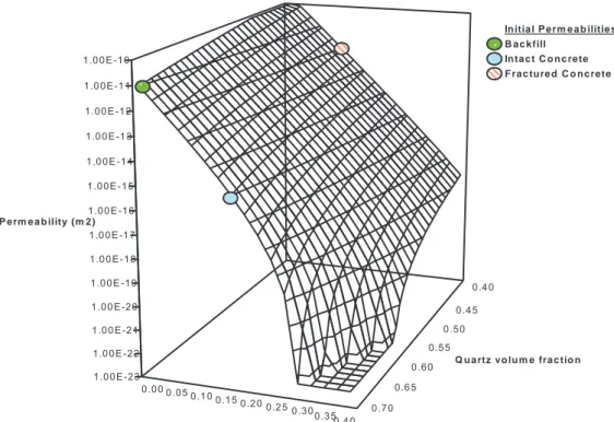
3.4.2 A Kozeny-Carmen relation for composite media

For the current study, we wish to study composite media comprising concrete and backfill regions. The backfill will be modelled as being entirely comprised of quartz particles and the total porosity of the backfill is initially 0.3. The concrete regions will initially be composed of cement and aggregate, with quartz acting as the aggregate material. The initial total volume fraction of the aggregate in the model is 0.7 (see Section 3.1), hence there is the same concentration of quartz in both the backfill and concrete regions. Since the Kozeny-Carmen relation only permits one parameter that describes the geometry of the media, a separate relation will have to be constructed in the backfill and concrete regions.

In the backfill, the reference permeability is 1e-11 m2 at the reference porosity 0.3.

Hence the parameter C in the backfill region will be

( )(

)

θ

θ

θ

In the concrete, the reference permeability is 1e-15 m2 at the reference porosity 0.125.

Hence the parameter C in the concrete region will be

13 10 92 . 3 × − = concrete C m2.

Since the concrete region can be considered to be equivalent to the backfill region but with cement filling some of the pore space, we might expect that if the cement phase were to be dissolved entirely the permeability of (what was originally) the cement