Department of Wildlife, Fish, and Environmental Studies
Habitat selection in moose and roe deer
– A third order comparison
Habitatval hos älg och rådjur – En jämförelse av tredje
ordningen
Irene Hjort
Habitat selection in moose and roe deer – A third order
comparison
Habitatval hos älg och rådjur – En jämförelse av tredje ordningen
Irene Hjort
Supervisor: Tim Hofmeester, Swedish University of Agricultural Sciences, Department of Wildlife, Fish, and Environmental Studies Assistant supervisor: Wiebke Neumann, Swedish University of Agricultural Sciences,
Department of Wildlife, Fish, and Environmental Studies
Examiner: Tim Horstkotte, Swedish University of Agricultural Sciences, Department of Wildlife, Fish, and Environmental Studies
Credits: 30 credits
Level: Second cycle, A2E
Course title: Master thesis in Biology
Course code: EX0937
Programme/education: Management of Fish and Wildlife Populations
Course coordinating department: Department of Wildlife, Fish, and Environmental Studies Place of publication: Umeå
Year of publication: 2019
Title of series: Examensarbete/Master's thesis
Part number: 2019:19
Online publication: https://stud.epsilon.slu.se
Keywords: GPS, camera trapping, habitat selection, order of selection, Alces alces, Capreolus capreolus, Brownian bridge kernel method
Ungulates are important animals in Swedish culture and economy, yet they are considered to cause considerable damage on forests to the disadvantage for the forest industry. At the same time, the forest industry is one of the reasons for the increased carrying capacity of moose and roe deer. Different factors affect the behaviours that cause the animals to inflict damage on the forest, but a main reason is access to browsing. The selection of habitat oc-curs on different spatial scales and this work looked closer on the selection at the 3rd order,
selection of habitat within the home range. The data that was used came from GPS collars from 7 female moose and 17 female roe deer that were tagged within the area of Nordma-ling in northern Sweden as well as from camera traps within this area. The GPS data was analysed using Brownian bridge kernel method to receive the utility distribution and home range of the animals. Thereafter the data was connected to the ground cover map allowing a comparison of the usage of different types of habitat using a logistic regression. The GPS data was analysed for the full year, but also sectioned into the periods when the animals were expected to fawn, the rutting period, winter and the full year but excluding fawning, rutting and winter. The results showed for high usage of decidious trees for the full year in both moose and roe deer, while both groups seemed to avoid water. Moose also selected for clear-cuts throughout the year with an increase during winter. Urban areas showed for a higher usage than were expected for by roe deer. Rutting season increased the usage of ara-ble land in moose while fawning season increased the usage of clear-cut areas by roe deer. The camera trapping data was also connected to the ground cover map and thereafter ana-lysed with a Poisson regression. These results confirmed the high usage of decidious forest but contained high standard errors, likely as a result of low amounts of data. They also covered less habitat types as an effect of the sampling method. To benefit the forest indus-try, further studies would be needed on how the animals behave within the different habi-tats. However, the access to forage seemed to be a driving factor in the habitat selection with the exclusion of the rutting season in moose and the fawning season in roe deer.
Keywords: GPS, camera trapping, habitat selection, order of selection, Alces alces,
Capreo-lus capreoCapreo-lus, Brownian bridge kernel method
Klövdjur är viktiga inom såväl svensk kultur som ekonomiskt, trots det anses de orsaka stor skada på skogen som i sin tur är till nackdel för skogsbruket. Samtidigt är en av orsakerna till de ökade populationerna av älg och rådjur skogsindustrin. Olika faktorer påverkar de beteende hos djuren som anses skada skogen, men en viktig faktor är tillgången till foder. Habitatval sker på olika spatiala skalor och det här arbetet har sett närmare på habitatval av den tredje ordningen, habitatval inom ett djurs hemområde. Data som insamlades kom från GPS-halsband från 7 älgkor och 17 rågetter som var märkta i området av Nordmaling som är beläget i norra Sverige samt från kamerafällor inom samma område. Data från GPSerna analyserades med Brownian bridge kernel method för att få fram hemområden och nyttjan-det av områden inom nyttjan-detta hemområde, därefter sammankopplades data med en karta över marktäcket för att få fram en jämförelse av nyttjandet av olika habitat med hjälp av logistisk regression. GPS-data analyserades för hela året, men också uppdelat i perioder för när djuren förväntades kalva, vara i brunst, för vintern och för hela året men med uteslutande av kalv-ning, brunst och vinter. Resultaten visade på ett högt nyttjande av lövskog över hela året för både älg och rådjur medan båda grupperna verkade undvika vatten. Älgkorna valde också kalhyggen under hela året men med en ökning under vintern. Bebyggda områden visade på ett större nyttjande än vad som förväntades hos rådjur. Brunsten ökade älgkornas nyttjande av jordbruksmark medan kalvningen ökade rådjurens nyttjande av kalhyggen. Data från ka-merafällorna sammankopplades också med data över marktäcket och analyserades med en Poisson regression. Resultaten bekräftade det höga nyttjandet av lövskog men innehöll höga medelfel, sannolikt som effekt av den låga mängden data från kamerafällorna. De täckte också färre habitattyper som en effekt av metoden för datainsamling. För att gynna skogsin-dustrin behövs ytterligare studier som visar hur älg och rådjur beter sig inom olika habitat, men tillgången till foder tycks vara en drivande faktor då det kommer till habitatval med undantag för vid brunsten hos älgkorna och vid kalvningen hos rågetterna.
Nyckelord: GPS, kamerafällor, habitatval, val av ordning, Alces alces, Capreolus capreolus,
Brownian bridge kernel method
1 Introduction 5 2 Method 8 3 Result 12 3.1 Moose 12 3.1.1 Camera data 12 3.1.2 GPS data 13 3.2 Roe deer 18 3.2.1 Camera data 18 3.2.2 GPS data 19 4 Discussion 23 4.1 Moose 23 4.2 Roe deer 24
4.3 Comparing GPS and camera trapping data 25
4.4 Conclusion 26
Referenslista/References 27 Tack/Acknowledgements 30
Innehållsförteckning/Table of contents
Ungulates are important nature resources, ecologically, economically and cultur-ally. Yet, todays’ populations of ungulates in Sweden are reckoned to cause con-siderable costs for the forest industry (Blenow & Sallnäs 2002; Ezebilo, Sand-ström & Ericsson 2012), even if different interest groups differ on the extent of the damage (Ezebilo, Sandström & Ericsson 2012). Moose (Alces alces) and roe deer (Capreolus capreolus) are important game species in Sweden and the acceptance for damage caused by these species is higher among hunters than among forest owners (Ezebilo, Sandström & Ericsson 2012), even so they are considered to be the biggest cause of damage on the forests, mainly because of dense populations (Bergquist 2017).
The carrying capacity for these animals has increased as an effect of modern for-estry (Kaien, 2006). Forfor-estry increases the number of shoots available to browse, but at the same times reduce bilberry that is important forage due to removal of older forest (Wam, Hjeljord & Solberg, 2010, Bergquist et al. 2009). This might cause difficulties in the decision-making process for management of moose and roe deer as well as in management decisions for forestry. In forestry, the decisions to plant less suitable tree species for the local habitat is a method used as an effort to avoid browsing damage caused by moose and roe deer (Kalén 2006), which is also considered a reason for the low interest in planting deciduous trees (Rytter, 2014). The degree of browsing damage is dependent on the size of the ungulate population as well as the available amount of forage (Blenow & Sallnäs 2002). Ezebilo, Sandström & Ericsson (2012) saw that the more energy that was spent on improving the moose habitat, the less severe the browsing damages were, and they concluded that a more holistic view in the management design would be beneficial for forestry. A holistic view would allow for creating forage in habitat that is lack-ing food supply, but otherwise is favorable (Bergqvist et al. 2018), as well as in-creased knowledge about selection of habitat would benefit for future decision making (Edenius et al. 2002).
Selection of habitat occurs at spatial (van Beest et al. 2010) as well as temporal scale (Street, Rodgers & Fryxell 2015; Neumann et al. 2018). Habitat selection at spatial scale can be divided into four orders according to Johnson (1980) and each scale is depending on the order above to be fulfilled. The first order concerns the geographical range/distribution of the species. The second order describes the
home range of an individual or a group and the third order of selection is the habi-tat selection within the home range. Finally, the fourth order of selection is the us-age of microhabitats within the habitat of a given animal or group. The habitat can be interchangeable if the different habitats fulfill the same purpose for the animal (e.g. food and /or shelter such as woodland and hedgerows could be for roe deer ( Morellet et al. 2011)).The selection of habitat is dependent on different factors, e.g., such as disturbance (Street et al. 2015), predation (Street et al. 2015; Decesare et al. 2014), and temperature (Street, Rodgers and Fryxell, 2015), but a main factor is access to forage (van Beest et al. 2010).
Moose and roe deer are both browsers that utilize a range of different habitats. Dif-ference in response to abiotic and biotic factors might differ between and within the species and factors such as sex and age contribute to these differences (Dussault et el. 2005; William et al. 2018). Kjellander et al. (2004) suggest that many of the differences seen in the home range selection in roe deer is an effect of the social and territorial systems that occur within the roe deer population. The se-lection at different orders (Johnson 1980) can vary. In moose, at the 2nd order, the selection of home range, animals selected quality over abundance, while at the 3rd order, when selecting habitat within the home range, they selected abundance over quality (van Beest et al. 2010).
Increased knowledge in the selection of habitat can be achieved with the help of modern technology and deeper understanding for the selection patterns for e.g., of moose and roe deer.
Various methods have been used to estimate the whereabouts of animals (Måns-son, Andrén & Sand 2011) and they all build on the assumption that the collected data is representative for the area that is researched. These methods allow us to collect information about the animals’ selection of habitat. Global positioning sys-tems (GPS) allows collection of a high amount of data and can give knowledge of the animals’ whereabouts with high precision (Månsson, Andrén & Sand 2011) this has opened for new ways to study them. However, the animals that are col-lared are often within a limited area, which makes the collected data representative only for a local population or build on the assumption that the subsample is repre-sentative for the whole population. GPS collars are also dependent on the function-ality of the battery and this can affect the time and the interval that the data can be collected. Yet, the data that is collected with GPS can be used to connect animal behavioral to individual features. Another recently developed method is camera trapping.
During recent years, wildlife cameras have become a more easily available tech-nique allowing higher quality on the data that is collected, which has led to an in-crease in the use of camera traps (Burton et al. 2015). As for the GPS technique, camera traps open for new methods of collecting information about animals. It is a noninvasive method that is cheap when it comes to collecting data and good to use in challenging settings such as dense forests where it is hard to directly observe an animal. Species data collected from camera traps, however can differ in their de-tectability (Sollmann et al. 2012). In summary, Hofmeester et al. (2018) identified 40 factors that could be affecting the detectability when using camera traps. For an animal to be detected, it needs to select the habitat where the camera is in the 1st
to 4th order. In addition, the animal needs to be detected by the camera and possi-ble to identify from that photograph (Hofmeester et al. 2018).
With my study, I intend to find out how habitat selection occur within the home range for moose and roe deer in north of Sweden over the year at the 3rd order in relation to different land types (such as arable land, clear-cuts and coniferous for-est). The usage of GPS collars allows me to collect data in high detail for a few an-imals to a high expense, while camera trapping data are less invasive to a lower cost, but do not give the same quality of information on a specific animal. There-fore, I compare these methods to see if it would be reasonable to use the cheaper camera trapping data when studying 3rd order habitat selection.
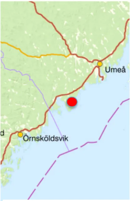
I used GPS collar data from 7 moose and 17 roe deer collected between February 2017 and May 2018 and March 2017 to May 2018, respectively within the Beyond moose project (Neumann et al. 2018), in the area of Nordmaling municipality in northern Sweden (Figure 1). The GPS data were gathered at a high interval the first three months collecting datapoints once every hour, and thereafter at a rate of every third hour for the rest of the period that the animal wore the GPS. I selected datapoints that were taken within 5 minutes from the full hour and from those se-lected out the datapoints that where taken every third hour, beginning at midnight, 03, 06, 09, 12, 15, 18, 21 for all the time that the animals where GPS tagged to make it easier to compare the data over the full year. This way I only had data-points that were taken within 5 minutes from midnight, 03 and so on. Spatial points were generated from the spatial data in the original file into a form of x and y coordinates
.
For the analysis, I then used the Brownian Bridge kernel method. The burst of the animal move-ments was calculated with the function as.ltraj within the kernelbb package. I used the liker function to calculate sig1 as the speed of the ani-mals and set sig2 to 20 as an estimate of the im-precision of the relocations. (Calenge, 2006) I thus used the spatial points that were generated previously to create a grid where I could apply the Brownian Bridge kernel method. The Brown-ian Bridge kernel method accounts for the time that passed between the animal single movement steps, and thereby considers autocorrelation among positions as often present in GPS loca-tions. This allows for an estimate of the likeli-hood of animal being at a given place and from that estimate it is possible to calculate utilization distribution. The grid size was set to the resolu-tion of 500 cells. From the result of the Brownian
2 Method
Figure 1. Nordmaling, the area
where the camera data where col-lected and the animals were collared is pointed out with a red mark.
Bridge kernel method I could estimate 95%, 75% and 50 % home range and utility distribution were extracted.
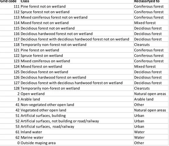
I then tested if there was a correlation between the probability of use, as estimated from the utility distribution, and different habitat types. I used” Nationella
marktäckedatan” (NMD), a map containing spatial information on the habitats in Sweden to extract habitat types. Due to the large number of classes, I reclassified biotopes that were available in NMD into 10 different habitat classes (Table 1). The logistic regression allows me to analyse correlation between a continues (amount of usage) and a categorical (habitat type) variable (Samuels et al. 2016). To enable easy comparison, I used coniferous forest as the intercept in the logistic regression model since I expected both moose and roe deer to spend time in this vegetation type. In addition, I also used a used a post-hoc Tukey test to test for dif-ferences between the habitat classes, e.g. coniferous forest was not used as inter-cept instead al classes were compared to one another.
Table 1. The classes from NMD and what they were reclassified to.
After running the analysis for the full period, I divided the data into different sea-sons to test if there were any differences in habitat selection as an effect of differ-ent natural evdiffer-ents. The winter season were set according to weather data from
Grid code Class Reclassifyed to
111 Pine forest not on wetland Coniferous forest 112 Spruce forest not on wetland Coniferous forest 113 Mixed coniferous forest not on wetland Coniferous forest 114 Mixed forest not on wetland Mixed forest 115 Decidious forest not on wetland Decidious forest 116 Decidious hardwood forest not on wetland Decidious forest 117 Decidious forest with decidious hardwood forest not on wetland Decidious forest 118 Temporarily non‐forest not on wetland Clearcuts 121 Pine forest on wetland Coniferous forest 122 Spruce forest on wetland Coniferous forest 123 Mixed coniferous on wetland Coniferous forest 124 Mixed forest on wetland Mixed forest 125 Decidious forest on wetland Decidious forest 126 Decidious hardwood forest on wetland Decidious forest 127 Decidious forest with decidious hardwood forest on wetland Decidious forest 128 Temporarily non‐forest on wetland Clearcuts 2 Open wetland Natural open areas 3 Arable land Arable land 41 Non‐vegetated other open land Other 42 Vegetated other open land Natural open areas 51 Artificial surfaces, building Urban 52 Artificial surfaces, not building or road/railway Urban 53 Artificial surfaces, road/railway Urban 61 Inland water Water 62 Marine water Water 0 Outside maping area Other
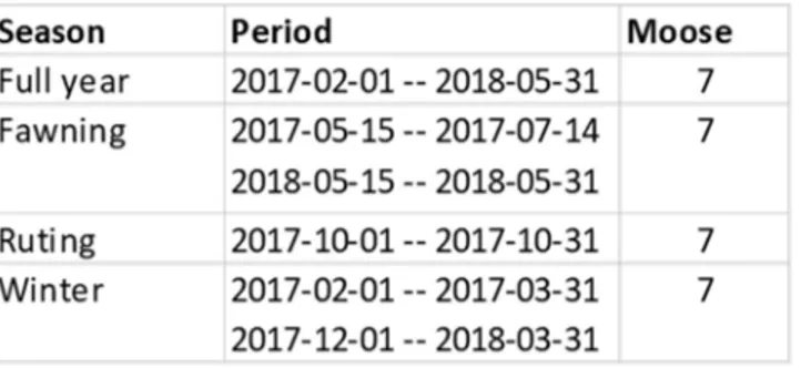
SMHI (www.smhi.se). For rutting and fawning the periods described by Bjärvall & Ullström (2010) were used for moose (Table 2) and roe deer (Table 3)
Table 2. The periods that were used for moose and the amount of moose that I was able to use in
each period.
Table 3. The periods that were used for roe deer and the amount of roe deer that I was able to use in
each period.
The camera trapping data that I was able to use for this study were collected at Jä-rnäshalvön, a peninsula in the Baltic Sea in northern Sweden (63° 32' N, 19° 41' E) that is in Nordmaling municipality (Figure1). The peninsula is a c. 200-km2 and
was divided into 11, 4 km long, transects that were evenly distributed over the area. For each transect, cameras were deployed at 18 pre-selected locations with 100 m between the locations. This resulted in 198 camera sites but 5 of those were excluded of from varying causes resulting in data from 193 cameras. The cameras were set up at the tree closest to a randomized GPS point within the transect and attached facing north to avoid direct sunlight into the camera lens. The cameras were also set at a level 60 cm above and parallel to the ground/snow cover. When triggered the cameras tock a series of 10 pictures. The cameras where then moved within the transect after 6-10 weeks to next randomized point. This study resulted in a sampling effort of 10,491 camera-trap days that were distributed over 382 days. From this the data in the pictures where aggregated to passages, if the pic-tures where taken within 5 minutes from each other they were considered the same animal or group of animals. From these passages the amount of moose and roe deer where counted as well how many days the camera been active. This data could then be used as the base of a Poisson regression that modelled the numbers of animals as a function of the vegetation class and only used full numbers. In the
Poisson regression I used the offset function so that the analyse tock into consider-ation that the cameras where used different amount of days.
All data was analysed in R version 3.5.3 mainly using package” adehabitatHR”, ”sp” ,”maptools”, ”rgdal”, ”raster” as well as ”multcomp”.
3.1 Moose
3.1.1 Camera data
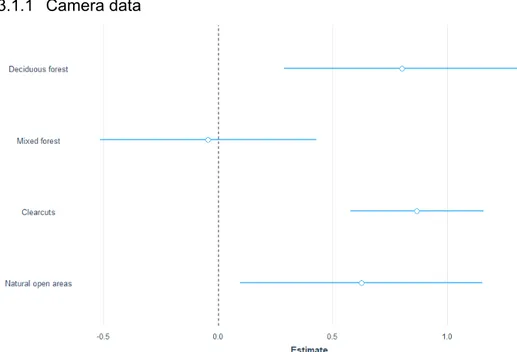
Figure 2 Estimates for moose over the full year with data from the camera traps where the different
classes is compared to coniferous forest (0.0). The blue lines represent the standard error.
I used data from 193 camera locations with 263 moose observations to test for a correlation between moose passage rates and different habitat types. Moose pas-sage rates on the cameras were higher in deciduous forest (est 0.8, z-value 3.1, p-value 0.002) and clearcuts (est 0.9, z-p-value 5.8, p-p-value 0.0001). Natural open ar-eas also had a higher passage rate (est.0.6, z-value 2.3, p-value 0.02) and were more likely to be used by moose compared to coniferous forest (Figure 2). The post-hoc test for camera data showed a higher passage rate in clearcuts compared
to coniferous forest (est 0.9, z-value 5.8, p-value <0,001) and in clearcuts com-pared to mixed forest (est 0.9, z-value 3.9, p-value 0.001). Deciduous forests had higher passage rates (est 0.8) compared to clearcuts (z-value 3.1 p-value 0.02). Passage rates were higher in deciduous compared to mixed forest, but with a lot of variation (est -0.84, z-value -2.6, p-value 0.07975).
3.1.2 GPS data
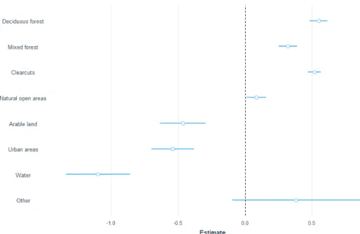
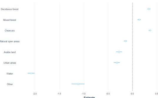
Overall, I had selected 22964 observations that fulfilled the requirements stated in the method, divided over 7 individuals of moose, resulting in an average of 3280.6 positions ± 785.5 per individual, in the analysis of moose habitat selection. Annu-ally, moose preferred deciduous forest, clearcuts and mixed forests above conifer-ous forest. The deciduconifer-ous forest was 1.7 times more likely to be used (z-value 15.7, p < 0.0001), clearcuts 1.68 (z-value 21.2, p < 0.0001) and mixed forest 1,37(z-value 9, p < 0.0001). The natural open areas were just slightly more used (1.1 times more used than coniferous forest) and had a lower significance (z-value =2.3, p-value 0.02). Arable land, urban areas and water where all less used by moose in comparison with the coniferous forest (Figure 3).
In the post-hoc test, I found that deciduous forest was the most used vegetation by moose, but the result was not significant when decidious forest was compared to clearcuts (z-value 0.9, p-value 0.9). Over the full year the moose also selected clearcuts above mixed forest and mixed forest above arable land. Moose clearly avoided water
Figure 3 Estimates for moose over the full year where the different classes are compared to
During winter (7697 GPS observations), moose showed a strong selection for clearcuts (z-value 21, p-value <0.0001) and was 2.3 times more likely to be found on those than in the coniferous forest. Mixed forest was selected 1.7 times more often than coniferous forest, decidious forest 1.6 natural open areas 1.2. (Figure 4) Both water and the category other were less used than coniferous forest, especially water was negatively selected and the difference between these categories is con-firmed in the post hoc test (z-value 12, p-value <0.001) where other is selected 3.7 times more often than water.
Figure 4. Estimates for moose during winter with data from the GPS where the different classes is
During rutting season, I analysed 1470 observations on moose. My results did not suggest any differences in utilization between neither deciduous or mixed forest compared to the coniferous forest. The class that I found were most used where arable land that moose selected 2.1 times more often than coniferous forest (z-value 21.9, p-(z-value <0.0001). Clearcuts, natural open areas and urban areas are slightly less used during this period. Class other had a very low usage and a high uncertainty. (Figure 5)
The post hoc test confirm that arable land is selected in front of other vegetation types during the rut.
Figure 5. Estimates for moose during rut with data from the GPS where the different classes are
During the time when moose where expected to give birth, I analysed 4041 obser-vations. Decidious forests and clearcuts are strongly selected for above coniferous as well as slight preference for mixed forests while the arable land, natural open areas, urban areas, water and other areas is significantly less selected for than clearcuts in the logistic regression analyse. (Figure 6)
The post hoc test confirmed that clearcuts is significantly selected for compared to all types of vegetation except for decidious forest that was equally selected for (es-timate 0.01, z-value 0.7, p-value 0.99). Class other were 1.7 times more used than water (z-value 13.9, p-value <0.0001) but less than urban areas (0.3 times the us-age of urban areas, z-value -31.2, p-value <0.0001).
Figure 6. Estimates for moose during fawning with data from the GPS where the different classes are
I also looked at periods over the year when the moose wasn’t expected to be di-rectly impacted by calving, the rut or winter conditions. Excluding observations from those periods, I had 9756 observations left for analysing. I found that be-tween the calving, rutting, and winter season, moose showed higher usage of de-cidious forest, mixed forest and clearcuts than for coniferous forest while all other classes were less used. (Figure 7)
The post hoc test shows that clearcuts was selected for prior to other classes but the result where not significant between clearcuts and decidious forest (p-value 0.88984). Decidious forest where preferred to coniferous forest, mixed forests as well as other classes except clearcuts, and thereafter mixed forest was selected for, all with a p-value of <0.001. Water was negatively selected for.
Figure 7. Estimates for moose over the full year but with fawning, rut and winter season excluded,
data from the GPS where the different classes are compared to coniferous forest (0.0). The blue lines represent the standard error.
3.2 Roe
deer
3.2.1 Camera data
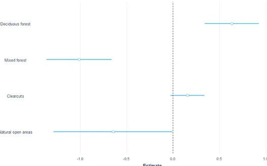
The camera trapping data for the roe deer where based on data from 193 camera locations with 658 observations of the GPS tagged roe deer. Here I saw that decid-ious forest were selected with an estimate of 0.6 more often than coniferous forest (z-value 4.2, p-value< 0.0001). Clearcuts where used more often than coniferous forest but were not significantly different (est 0.2, z-value1.7, p-value 0.09). Since no cameras were placed in arable land or urban areas values for those can’t be pre-sented in this result. (Figure 8)
The post hoc test confirmed the Poisson regression.
Figure 8. Estimates for roe deer over the full year with data from the camera traps where the
3.2.2 GPS data
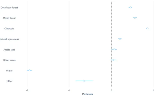
For roe deer, I analysed 23339 observations with an average of 1372.9 ± 767.3 (n=17 individuals) and found that roe deer annually showed a strong preference for decidious forest (1.7 times more often than coniferous forest z-value 27.2, p-value <0.0001). Animals also had a strong selection for the class other that was equally selected to decidious forest (1.7 times more often than coniferous forest z-value 2.2, p-z-value 0.03) Mixed forests, natural open areas where all used more than coniferous forest while usage of clearcuts arable land and water were lower. (Figure 9)
The post hoc test showed that urban areas where selected above clearcuts, conifer-ous forests, water, arable land (p-values <0.001) while decidiconifer-ous forests where se-lected before urban areas (p-value <0.001). The post hoc also confirmed that the selection for class other where not significantly different from decidious forest (z-value 0.022, p-(z-value 1).
Figure 9. Estimates for roe deer GPS data over the full year where the different classes are
During the winter (10070 observations), roe deer used arable land most (2.1 times more often than coniferous forests, z-value33.4, p-value < 0.0001) and thereafter mixed forests and decidious forests. The only classes that were less used than co-niferous forests were water and other. Closest to coco-niferous forests in usage where natural open areas (1.03 times more used, z value 2.3, p-value 0.0236) and clear-cuts (1.1 times more used, z-value 7.8, p-value < 0.0001). (Figure 10)
The post hoc test shows for a high usage of arable land confirming the logistic re-gression.
Figure 10. Estimates for roe deer during winter with data from the GPS where the different classes
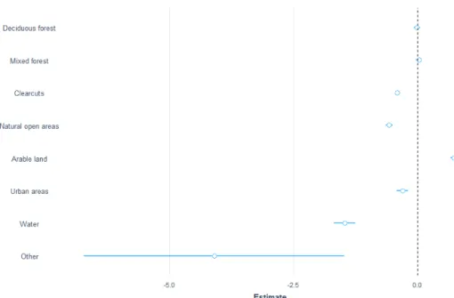
During rutting period (953 observations from 4 individuals), roe deer preferred de-cidious forest (2.7 times more used than coniferous forest, z-value 30.1, p-value <0.0001), clearcuts (1.6 times more used than coniferous forest, z-value 18.5, p-value <0.0001), and natural open areas (1.3 times more used than coniferous for-est, z-value 10.3, p-value <0.0001), that are all selected above coniferous forest while mixed forest and urban areas is slightly less selected than coniferous forest. Other, arable land and water are all significantly less used (p-value <0.0001). The post hoc test showed no significant difference between coniferous forest and mixed forests or urban areas in this period and suggests that there is no significant difference between mixed forests and urban areas.
During fawning period (includes 5315 observations), roe deer had a high usage of clearcuts, decidious forests, arable land and natural open areas selected 1.8, 1.8, 1.6 and 1.4 times more often than coniferous forests in the logistic regression. Ur-ban areas are almost equally selected for (1.1 times more often than coniferous forest, z-value 2.9, p-value 0.004) while mixed forests, other and water where less selected for. The post hoc test gives results that confirm the logistic regression in exception of a non-significant result when comparing urban areas and coniferous forest (z-value 2.9, p-value 0.07). (Figure 11)
Figure 11. Estimates for roe deer during fawning with data from the GPS where the different classes
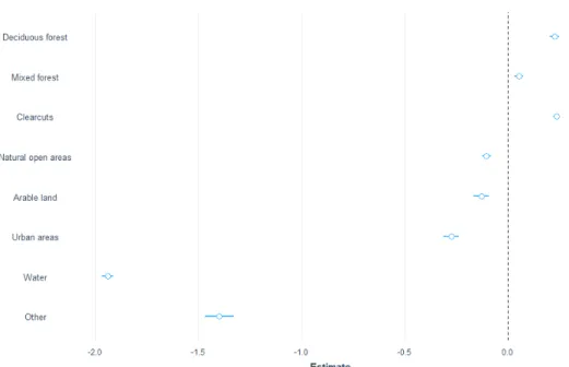
When excluding fawning, rutting season and winter there were 7455 observations left. Here I found that roe deer had a higher usage of arable land (2.8 times more often than coniferous forest, z-value 51.2, p-value <0.0001), decidious forest, (2.5 times more often than coniferous forest, z-value 67.9, p-value <0.0001) urban ar-eas (1.6 times more often than coniferous forest, z-value 22.5, p-value <0.0001) and other (1.6 times more often than coniferous forest, z-value 5.9, p-value
0.0001) in comparison to coniferous forest. Mixed forest clearcuts and water were all less used than coniferous forest while natural open areas showed no significant difference. The post hoc test confirms the result in the logistic regression. (Figure 12)
Figure 12. Estimates for roe deer over the full year but with fawning, rut and winter season excluded,
data from the GPS where the different classes are compared to coniferous forest (0.0). The blue lines represent the standard error.
As was expected, habitat selection varied over the year for both moose and roe deer and the causes for these variations are likely to be the effect of many interact-ing factors such as access to forage (Wam, Hjeljord & Solberg, 2010, van Beest et al. 2010, Samelius et al. 2013), temperatures (van Beest, Van Morter & Milner, 2012, Street, Rodgers & Fryxell, 2015, Månsson, Andrén & Sand, 2011), and hu-man activities (Bonnot et al. 2013, Street et al., 2015, ). The camera trapping data coincided with the data from the GPS collars when it came to what seemed like the strongest preferences among the animals, while looking at habitats that were less selected for there were more difference between the results.
4.1 Moose
Over the full study period moose, as could be expected as an effect of greater ac-cess to forage, at the 3rd order of selection preferred decidious forest, clearcuts and mixed forest over coniferous forest. Over the full year mixed forest seems to be less used than both decidious forests and clearcuts. The fact that natural open areas were used in a similar amount to the coniferous forest I see as likely to be an effect of the same amount of available food therein or the same usage of the habi-tat as a transit area. During the winter I saw an increase in the usage of areas that been clear-cut recently which coincides with previous knowledge about moose browsing preference (van Beest et al. 2010, Bergqvist et al. 2018). Moose prefera-bly browse on rowan (Sorbus aucuparia), aspen (Populus tremula) and sallow (Sa-lix caprea) in the north of Sweden during the summer months (Wam, Hjeljord & Solberg, 2010), but since those are not available during winter pine (Pinus syl-vestris) becomes an important food source and those are easily accessible in young forests and recently clear-cut areas.
During the rut there was a clear change in the behavioural patterns of the moose in this study, and they clearly selected for arable land. This suits my second hypothe-sis that certain events such as the rut will override the search of forage, still, an-other reason for this could be that certain crops are still standing on the field offer-ing high energy forage. Another reason could be that huntoffer-ing season begins
proximately a month before the rut (www.jagareforbundet.se) and this possibly al-tered the moose movement patterns, but this were shown in a study by Neumann, Ericsson and Dettki (2009) to not be the case for the moose population. However, they saw that individuals could be affected by hunting and since the study con-struct on so few individuals (7) it might be so that the presence of one or a few in-dividuals in this dataset that show a response has a big impact on the result. As for my third hypothesis moose never seemed to select for urban areas but the result didn’t suggest that those areas were avoided either. On contrary I would say that avoidance was true for water. Still, both water and urban areas are compara-tively rare within the study area and therefore these results would need to be tested over a bigger area with bigger amounts of animals to say something for certain. Looking at the moose GPS data, in comparison with the camera trap data, that had a lot fewer observations, the higher usage of mixed forests was missing out and the result were not significantly different from coniferous forest. I could still see a strong preference for decidious forest and clearcuts among moose. Contradicting the result from the GPS data, natural open areas where more used in the camera trap data, one cause for this difference could be the few observations in the camera trap data, another could be the that the camera trap photograph an animal even if it is just passing and gives this information the same value as a longer stay while the GPS data is less likely to send out a signal in areas where the animal is only pass-ing. Still I would argue that the likeliest cause would be the difference in detecta-bility by the camera trap in different settings since it would be reasonable to as-sume that an animal is easier to detect by the camera’s sensor in an open area then in a forest, this is described to be a relevant factor by Hofmeester et al. (2018). Comparing the result from the camera trap data with the result from the GPS data over the full year the strongest selected habitats, deciduous forest and clearcuts, were approximately equally selected for in both methods for moose.
4.2 Roe
deer
Roe deer showed a greater variation in habitat selection over different seasons. Over the full year, I could see a preference for deciduous forest but also a high us-age of the class other, although there was a high standard error for that class. The high usage of decidious forest was confirmed by the Poisson regression of the camera trapping data. In winter there was a high usage of arable land, that habitat had also a high usage during fawning, but deciduous forest showed for almost the same amount of data points. The high variation in habitat selection might be the result of the roe deer’s pursuit of high-quality forage throughout the year an coin-cides with Moser, Schültz & Hindenlang (2006) that suggest that roe deer alter their forage selection to find the highest quality food.
This pursuit of high-quality forage could also explain why I didn’t see any clear changes in habitat selection during fawning except for an increase in the usage of clear cuts. According to Vospernik & Reimoser (2008) roe deer preferable reside
in areas that quite recently been clear cut since it provides food as well as cover-age. This could explain why roe deer increased their usage of clear-cuts during the fawning. However Samelius et al. (2013) suggested that quality of the habitat (and the available forage within) had bigger effect on roe deer than did the presence of lynx (Lynx lynx) and this could suggest that the access to forage might be more important than shelter and this could explain why there wasn´t that big change in usage for the other habitats. During rutting there was a strong selection for decidu-ous forest, but this result was constructed on datapoints from only four individuals and therefore contains a high uncertainty.
Unlike moose, roe deer often selected urban areas above coniferous forest contra-dicting Coulon et al. (2008) that suggested avoidance within 400 meters from buildings. Still the urban areas in the NMD might also cover areas above 400 me-ters from buildings and if so, there would be a positive effect above that distance and still possible to count as urban area.
The analyse of the GPS data for roe deer over the full year suggested that clearcuts were less used than coniferous forest while mixed forest was more used. This is contradicted by the result from the camera trap data that suggests that clearcuts is more used than both coniferous forest and mixed forest. This difference I result might be caused by random chance or by the setup of the camera. It is not possible to tell witch one has the “true” result for describing roe deer selection however, less dwelling in recently clear-cut areas is beneficial for regeneration of forest, therefore it would be relevant to ascertain if an increase of mixed forests is reduc-ing dwellreduc-ing in clear cut areas.
.
4.3 Comparing GPS and camera trapping data
Due to the type of data that are the result of the GPS trackers, with highly specific times for datapoint and no knowledge about what the animal is doing at a given time, it is possible that a low used forage is given the same value as a high used passing by area. The benefit of the camera trap data is that even at a low number of pictures, it is possible to say what the animal been doing at a given place and time. Even if the GPS gives a high knowledge about the whereabouts of one indi-vidual it gives limited information on the total use of a specific habitat. Camera traps on the contrary gives little or no information on animal movement (if it’s not possible to identify individuals from pictures (Sollman et al.2013), which rarely is the case with ungulates in Sweden) but gives good information on what the animal is doing in a specific habitat. The GPS studies the individual animals’ selection of habitat (Rempel et al. 1995), while the camera trap studies animals at a given habi-tat. Therefore, for the purpose of finding ways of a more sustainable forestry with less foraging damages the important question might be how a habitat is used, and thereby camera traps might be a good tool and a logical direction to continue in to
find the answer on how to improve methods of forestry to avoid foraging (Cara-vaggi et al. 2017).
However, there are places where it’s not reasonable to set up camera traps such as water due to the low usage of the habitat and urban areas due to the high number of pictures that would be taken on humans and thereby intrude on their privacy. In such areas GPS might be the only way to go to find out more, but either way it’s not likely to have a huge impact on forestry. Overall for the purpose of this study I would argue that the GPS data was best suited to answer the first three hypothesis. In this study there was a lot fewer datapoint in the camera trap data, and it held a higher uncertainty, thereby confirming my last hypothesis and this is likely to be the result since camera traps are highly dependent on the amounts of passing ani-mals and the number of cameras set up. Still, the overall result in both GPS data and camera trapping data showed for a high usage of deciduous forest and clear-cuts by moose and deciduous forest by roe deer. This suggests that to reduce dam-age on coniferous forest an increase of deciduous forest could be established as a preventive measure. But more studies would be needed in that specific matter.
4.4 Conclusion
Both moose and roe deer seemed to be very dependent on access to forage and that risks affecting forest in a way that might be considered to damage forest industry. The habitat that seemed most favourable over the year for both species where de-cidious forest while the most avoided habitat type where water, however a future study would likely benefit from observing usage of areas that is nearby water. Ef-fects on habitat selection driven by biological factors such as rut and fawning were seen in both moose and roe deer, but not always and the usage of urban areas were higher than expected, especially in roe deer. This suggests that the factors that drives the habitat selection by these ungulates in the area of Nordmaling needs fu-ture research and that it might be more complex than what was hypothesised in the beginning of this work.
For the future it would be relevant to more thoroughly examine the camera data to find out what animals are doing at the 4th order of selection, thereby pictures only used for passing through could be excluded and pictures where the animal is using a behaviour considered to damage the forest can be analysed. It would also be rele-vant to see difference of usage of forest of different ages, since it is reasonable to believe that young forest is under a higher predation pressure than older forest while old trees might be more exposed to behaviours such as pealing of the bark and antler rubbing. For this work I looked closer at the full year, the rut, the fawn-ing season and winter, this sectionfawn-ing could be done differently and would likely highlight different aspects the animals ecology in response to other abiotic and bi-otic factors.
Bergquist, J., (2017) Hjortvilt. I. Witzell, J. (2017). Skogsskötselserien 12 del 1, Skador på skog: 2nd edition. Jönköping: Skogsstyrelsen. pp 88-98 Available: https://www.skogsstyrel-sen.se/skogsskotselserien [2019-07-31]
Bergquist, J., Löf, M., & Örlander, G. (2009). Effects of roe deer browsing and site preparation on performance of planted broadleaved and conifer seedlings when using temporary fences. DOI: 10.1080/02827580903117420 Scandinavian Journal of Forest Research, 24(4), 308–317. https://doi.org/10.1080/02827580903117420
Bergqvist, G., Wallgren, M., Jernelid, H., & Bergström, R. (2018). Forage availability and moose winter browsing in forest landscapes. Forest Ecology and Management, 419-420, 170–178. https://doi.org/10.1016/j.foreco.2018.03.049
Bjärvall, A., Ullström, S. (2010). Däggdjur i Sverige: alla våra vilda arter. Stockholm: Bonnier fakta. Print
Blennow, K., & Sallnäs, O. (2002). Risk Perception Among Non-industrial Private Forest Owners. Scandinavian Journal of Forest Research, 17(5), 472–479.
https://doi.org/10.1080/028275802320435487
Bonnot, N., Morellet, N., Verheyden, H., Cargnelutti, B., Lourtet, B., Klein, F., & Hewison, A. (2013). Habitat use under predation risk: hunting, roads and human dwellings influence the spa-tial behaviour of roe deer. European Journal of Wildlife Research, 59(2), 185–193.
https://doi.org/10.1007/s10344-012-0665-8
Burton, A., Neilson, E., Moreira, D., Ladle, A., Steenweg, R., Fisher, J., … Boutin, S. (2015). RE-VIEW: Wildlife camera trapping: a review and recommendations for linking surveys to ecologi-cal processes. Journal of Applied Ecology. https://doi.org/10.1111/1365-2664.12432
Caravaggi, Anthony, Banks, Peter B., Burton, A Cole, Finlay, Caroline M. V., Haswell, Peter M., Hayward, Matt W., Rowcliffe, Marcus J. & Wood, Mike D. (2017). A review of camera trapping for conservation behaviour research. Remote Sensing in Ecology and Conservation, vol. 3 (3), pp. 109–122. https://doi.org/10.1002/rse2.48
Calenge, C. 2006. The package adehabitat for the R software: a tool for the analysis of space and habitat use by animals. Ecological modelling, 197, 516-519. Available: https://www.rdocumenta-tion.org/packages/adehabitatHR/versions/0.4.16/topics/kernelbb [2019-10-03]
Coulon, A., Morellet, N., Goulard, M., Cargnelutti, B., Angibault, J., & Hewison, A. (2008). Infer-ring the effects of landscape structure on roe deer (Capreolus capreolus) movements using a step selection function. Landscape Ecology, 23(5), 603–614. https://doi.org/10.1007/s10980-008-9220-0
Decesare, N., Hebblewhite, M., Bradley, M., Hervieux, D., Neufeld, L., & Musiani, M. (2014). Linking habitat selection and predation risk to spatial variation in survival. Journal of Animal Ecology, 83(2), 343–352. https://doi.org/10.1111/1365-2656.12144
Dussault, C., Ouellet, J., Courtois, R., Huot, J., Breton, L., Jolicoeur, H., & Kelt, D. (2005). Linking Moose Habitat Selection to Limiting Factors. Ecography, 28(5), 619–628. DOI:
10.1111/j.2005.0906-7590.04263.x
Edenius, L., Bergman, M., Ericsson, G., & Danell, K. (2002). The role of moose as a disturbance factor in managed boreal forests. Silva Fennica, 36(1), 57–67. https://doi.org/10.14214/sf.550 Ezebilo, E., Sandström, C., & Ericsson, G. (2012). Browsing damage by moose in Swedish forests:
assessments by hunters and foresters. Scandinavian Journal of Forest Research, 27(7), 659–668. https://doi.org/10.1080/02827581.2012.698643
Hofmeester, T., Cromsigt, J., Odden, J., Andrén, H., Kindberg, J., & Linnell, J. (2019). Framing pictures: A conceptual framework to identify and correct for biases in detection probability of camera traps enabling multi-species comparison. Ecology and Evolution, 9(4), 2320–2336. https://doi.org/10.1002/ece3.4878
Johnson, D.H. (1980). The Comparison of Usage and Availability Measurements for Evaluating Resource Preference. Ecology, vol. 61 (1), pp. 65–71 Ecological Society of America. DOI: 10.2307/1937156
Kaien, C. (2006). Deer Browsing and Impact on Forest Development. Journal of Sustainable For-estry, 21(2-3), 53–64. https://doi.org/10.1300/J091v21n02_04
Kjellander, P., Hewison, A., Liberg, O., Angibault, J., Bideau, E., & Cargnelutti, B. (2004). Experi-mental evidence for density-dependence of home-range size in roe deer (Capreolus capreolus L.): a comparison of two long-term studies. Oecologia, 139(3), 478–485.
https://doi.org/10.1007/s00442-004-1529-z
Morellet, N., Moorter, B., Cargnelutti, B., Angibault, J., Lourtet, B., Merlet, J., Ladet, S., Hewison, A. (2011). Landscape composition influences roe deer habitat selection at both home range and landscape scales. Landscape Ecology, 26(7), 999–1010. https://doi.org/10.1007/s10980-011-9624-0
Moser, B., Schütz, M., & Hindenlang, K. (2006). Importance of alternative food resources for browsing by roe deer on deciduous trees: The role of food availability and species quality. Forest Ecology and Management, 226(1), 248–255. https://doi.org/10.1016/j.foreco.2006.01.045 Månsson, J., Andrén, H., & Sand, H. (2011). Can pellet counts be used to accurately describe winter
habitat selection by moose Alces alces? European Journal of Wildlife Research, 57(5), 1017– 1023. https://doi.org/10.1007/s10344-011-0512-3
Neumann, W., Ericsson, G. (2018). Influence of hunting on movements of moose near roads. Jour-nal of Wildlife Management, 82 (5), 918–928. https://doi.org/10.1002/jwmg.21448
Neumann, W., Ericsson, G., & Dettki, H. (2009). The non-impact of hunting on moose Alces alces movement, diurnal activity, and activity range. European Journal of Wildlife Research, 55(3), 255–265. https://doi.org/10.1007/s10344-008-0237-0
Neumann W, Stenbacka F, Evans A, Arnemo JM, Widemo F, Ericsson G, Singh N och Cromsigt J. 2018. Årsrapport GPS-märkta älgarna och rådjur i Nordmaling 2017/2018; Rörelse, reproduktion och överlevnad. Sveriges Lantbruksuniversitet, 24pp
Rempel, Robert S., Rodgers, Arthur R. & Abraham, Kenneth F. (1995). Performance of a GPS Ani-mal Location System under Boreal Forest Canopy. The Journal of Wildlife Management, vol. 59 (3), pp. 543–551 The Wildlife Society. DOI: 10.2307/3802461
Rytter, L. (2014). Skogsskötselserien 9, Skötsel av björk, al och asp. Jönköping: Skogsstyrelsen. Available: https://www.skogsstyrelsen.se/skogsskotselserien [2019-07-15]
Samelius, G., Andrén, H., Kjellander, P., & Liberg, O. (2013). Habitat selection and risk of preda-tion: re-colonization by lynx had limited impact on habitat selection by roe deer. PLoS ONE, 8(9), e75469. https://doi.org/10.1371/journal.pone.0075469
Samuels, Myra L.., Witmer, Jeffrey A. & Schaffner, Andrew A. (2016). Statistics for the life sci-ences. 5th edition. global edition. Harlow: Pearson Education Limited.
Sollmann, Rahel, Mohamed, Azlan, Samejima, Hiromitsu & Wilting, Andreas (2013). Risky busi-ness or simple solution – Relative abundance indices from camera-trapping. Biological conserva-tion, vol. 159, pp. 405–412 Elsevier Ltd. http://dx.doi.org/10.1016/j.biocon.2012.12.025 Street, G., Rodgers, A., & Fryxell, J. (2015). Mid-Day Temperature Variation Influences
Seasonal Habitat Selection by Moose. The Journal of Wildlife Management, 79(3), 505–512. https://doi.org/10.1002/jwmg.859
Street, G., Vander Vennen, L., Avgar, T., Mosser, A., Anderson, M., Rodgers, A., & Fryxell, J. (2015). Habitat selection following recent disturbance: model transferability with implications for management and conservation of moose (Alces alces). Canadian Journal of Zoology, 93(11), 813–821. https://doi.org/10.1139/cjz-2015-0005
van Beest, F., Mysterud, A., Loe, L., & Milner, J. (2010). Forage quantity, quality and depletion as scale‐dependent mechanisms driving habitat selection of a large
browsing herbivore. Journal of Animal Ecology, 79(4), 910–922. https://doi.org/10.1111/ j.1365-2656.2010.01701.x
van Beest, F., Van Moorter, B., & Milner, J. (2012). Temperature-mediated habitat use and selec-tion by a heat-sensitive northern ungulate. Animal Behaviour, 84(3), 723–735.
https://doi.org/10.1016/j.anbehav.2012.06.032
Vospernik, S., & Reimoser, S. (2008). Modelling changes in roe deer habitat in response to forest management. Forest Ecology and Management, 255(3), 530–545.
https://doi.org/10.1016/j.foreco.2007.09.036
Wam, H., Hjeljord, O., & Solberg, E. (2010). Differential forage use makes carrying capacity equivocal on ranges of Scandinavian moose (Alces alces). Canadian Journal of Zoology, 88(12), 1179–1191. https://doi.org/10.1139/Z10-084
William, G., Jean-Michel, G., Sonia, S., Christophe, B., Atle, M., Nicolas, M., Pellerin, M., Clément, C. (2018). Same habitat types but different use: evidence of context-dependent habitat selection in roe deer across populations. Sci Rep, 8(1), 5102–5102.
A special thanks to my supervisors Tim Hofmeester and Wiebke Neumann for their great understanding that life happens and for sharing their high competence. And to grandma, because without her this work wouldn’t exist.
Thank you.