Software defined acoustic underwater modem

(1)

Software Defined Acoustic Underwater Modem

Jakob Lindgren

(2)

Abstract

Today many types of communication are employed on seagoing vessels, such as radio, satellite and Wi-Fi but only one type of communication is practical for submerged vessels, the acoustic underwater modem. The ”off-the-shelf” modems are sometimes difficult to update and replace, especially on a large submarine. But by separating the hardware from the signal processing and making the software modular more versatility can be achieved.

The questions that this thesis are asking are: is it possible to implement the signal processing in software? How small or large should the modules be? What kind of architecture should be used? This thesis shows that it is indeed possible to implement simple algorithms that can isolate a signal and read its content regardless of the hardware configuration. Calculations show that up to 13 kbps can be reached at a range of one kilometer. It is most practical to make the entire physical layer into one module and the size of the system could drastically change the type of architecture used.

(3)

Preface

This Master’s thesis from Jakob Lindgren is the final project for receiving the

Master’s degree in Robotics at M¨alardalen University in V¨aster˚as, Sweden.

It covers the basics of digital communication in the underwater channel as well as some simple algorithms for software defined communication. The purpose of this master thesis is to investigate how a software defined acoustic underwater communication can be implemented. This work was done at Saab Underwater Systems in Motala, Sweden, during the autumn term of 2010.

I hope this thesis can increase your knowledge of communications and software design and hopefully you will put this report away with more an-swers than questions. I would also like to take this opportunity to thank my thesis advisor, Ola Pettersson, for the help, questions and laughs given during this work.

(4)

Chapter 1 Introduction

1.1 Background

Saab Underwater Systems (SUS) has a long history of making underwater

vehicles including torpedoes, ROVs and AUVs. These ROVs and AUVs

are used in sea-bottom mapping, mine detection, the offshore industry and

even as a synthetic submarine target. In all these areas it is important

to communicate with the ROV or AUV by sending instructions or receiving data. Therefore, many of them feature some kind of wireless communication. One vehicle can have up to four ways to communicate: Wi-Fi, radio, satellite and an acoustic link.

Three of the communication links require that the vehicle has surfaced with the exception of the acoustic link. It uses sound waves to communicate and is capable to do so for several kilometers. However, the acoustic link is a very low speed communication system and often expensive and inflexible. These acoustic modems are usually bought ”off-the-shelf”, and replacing or upgrading them often implies a change of the entire unit.

Many steps in the acoustic communication can be made simpler, easier to maintain and easier to change or replace. Many of these improvements could also be implemented in software. This could, in turn, result in a system consisting of software connected to a set of speakers and microphones. The software could be easily changed and able to work in different environments and regardless of the hardware attached, thus making the communication system more versatile.

But some complexity is required to handle different environments which yields different problems. A shallow water environment [16, 5] may suffer heavily to echoes, which degrades the signal, and an AUV communicating with a boat can suffer severe Doppler effects. Some components of an

(7)

under-water communication link can be used regardless of the environment, such as compression or encryption, but some parts may not work at all. It would therefore be practical to make the software modular. This project is therefore aimed at investigating the difficulties of such a modular system.

SUS have for some time used a publish and subscribe middleware [13] to aid interprocess communication. It would therefore be favorable if the underwater communication were modular and could be connected using the same middleware. The modern communication protocols are generic and very modular in their nature. TCP can for example be used regardless of the lower protocol layers and the same is true with IP. This indicates that the layers themselves should not have any problem being separate modules. But an acoustic underwater modem needs a physical layer dedicated to the underwater channel. Can this layer be modular internally? The physical layer will therefore be the focal point of the project.

(8)

1.2 Project objectives and limitations

The interesting questions are:

• Is it possible to implement a working software modem without hardware

support?

• Is it further possible to make the system modular?

• If so, what kind of modules in the physical layer are required to make

a software modem work?

• What kind of modules in the physical layer are not required to make a

software modem work?

• How small or large should the modules be?

• Is a publish Subscribe middleware a viable solution for connecting the

modules?

• What bit rate can be achieved with such a modem?

There are several ways to answer these questions and one way is ”learning by doing”. This is the method that will be used and therefore a a refer-ence implementation will be constructed. This boils down to the following objectives:

• Perform a literature study of existing technology. • Implement a modem.

• Implement a simple channel simulator.

• Draw conclusions from the reference implementation about how

inter-connected the system is.

• Determine if a publish subscribe middleware is suitable for the

imple-mented system.

There are also some topics that will not be touched. This project will not focus on the hardware development, in fact it will be hardware independent. Nor will the project address covert communication.

(9)

Chapter 2 Acoustic underwater

communication

2.1 Network protocol structure

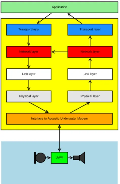
A common protocol structure for a network stack is the OSI model [23], or Open Systems Interconnection model. This model is used as a basis for the network topology. The network is assumed to have five basic layers, as illustrated in Figure 2.1.

Application layer is the top most layer. This layer is the user defined

application that can send and receive data through the underwater channel.

Transport layer is the interface between the application and the rest of

the protocol stack. This can include flow control, resending of data and acknowledge incoming packets.

Network layer is responsible for modifying the data blocks to a format

that the link layer can handle. It must cut large data blocks into

smaller ones and reassemble them later. It must be able to determine if an incoming packet is new or has been received before. It is also responsible for routing incoming packets.

Link layer manages the transmission between the modems, determining

where to send the frame in order to reach the end point. It also detects collisions and sometimes even avoids them.

Physical layer is the final layer before the frame is transmitted. The frame

(10)

Application Transport layer Network layer Link layer Physical layer Transport layer Network layer Link layer UWM Physical layer

Interface to Acoustic Underwater Modem

Figure 2.1: Structure of software defined acoustic underwater modem

must arrive at it’s destination undamaged. Erroneous frames need to be corrected or discarded. The frame may also need to be encrypted, scrambled or compressed.

The use of an underwater channel result in some changes in the layers. The ”off-the-shelf” transport layer can work well for the underwater channel. Some timing variable need to be changed though, as the propagation rate is significantly lower than common Ethernet or Wi-Fi.

Some consideration also need to be devoted to the fact that the underwa-ter channel is a multicast environment. Multicast implies that many nodes receives the same message. This could have an effect on the routing and retransmission algorithms.

The basic thing needed in a physical layer of a protocol stack for an acous-tic underwater modem is a modulation unit. Bits can not be transmitted into the water in raw form, they need to be modulated. There are several ways to modulate data, mentioned in section 2.7.

Before modulation some additional steps might be needed, for example if the message sizes are preferred to be small a compression algorithm might be in order. Two important steps are the Forward Error Correcting code and the interleaver. These two helps combat bit errors in the received messages.

(11)

Protection of data is some times a requirement for which an encryption unit can be added. According to [14, pg. 234], encryption should not pre-cede compression. Encryption would hide basic statistical characteristics of an uncompressed signal, such as spatial and temporal correlations, that are heavily exploited by compression algorithms.

2.2 Acoustic underwater modem

The word modem is a blend of the words modulator and demodulator [22]. This implies that it is a device that modulates a data stream into a waveform and demodulates a waveform back into a data stream. The word acoustic specifies that the modem uses sound to communicate and underwater implies that it transmits sound through the water.

2.3 Software driven modem

Most commercial acoustic underwater modems are hardware driven, the speakers and hydrophones are connected to circuitry that manages the com-munication. This can make the system efficient since the hardware can be constructed to match the properties of the equipment. But this solution lacks flexibility.

A Software driven modem can be changed without changing the hardware and vice versa. A software driven solution may however be bulkier since the modem needs some kind of computer to perform the necessary calculation. It may also need more power than a ”hardware” modem, due to the gen-eral purpose hardware of the computer, which can be a problem in a small, battery-powered application.

2.4 Underwater channel

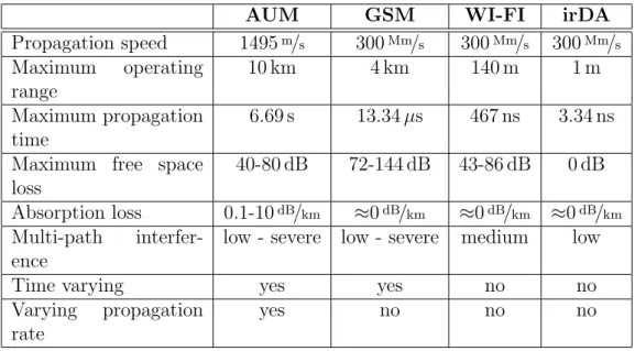
The underwater environment challenges the acoustic underwater modem [17] in several different ways that other communication systems does not need to consider. Table 2.1 illustrates some of the differences between an acoustic underwater modem(AUM) system, the cellular phone technology GSM, a Wi-Fi network and an infrared device. The table describes their maximum ranges, the time it takes to reach max range, loss parameters and other properties. Some of the parameters are taken from datasheets [11, 6] and

others are calculated. Note that some parameters are dependent on the

(12)

AUM GSM WI-FI irDA Propagation speed 1495m_/_s ₃₀₀Mm_/_s ₃₀₀Mm_/_s ₃₀₀Mm_/_s Maximum operating range 10 km 4 km 140 m 1 m Maximum propagation time 6.69 s 13.34 µs 467 ns 3.34 ns

Maximum free space loss

40-80 dB 72-144 dB 43-86 dB 0 dB

Absorption loss 0.1-10dB_/_km ≈0dB_/_km ≈0dB_/_km ≈0dB_/_km

Multi-path

interfer-ence

low - severe low - severe medium low

Time varying yes yes no no

Varying propagation

rate

yes no no no

Table 2.1: Comparison between four different communication technologies.

Free space loss This is the fact that sounds looses strength the further it

has to travel. A speaker at a conversion needs to speak up in order to be heard by the people in the back.

Absorption loss This is the simple fact that the signal looses strength the

longer it needs to travel through a medium. Imagine listening to the speaker from an adjoining room. The sound looses strength when it travels through the wall between the rooms. The loss can differ from one frequency to another.

Multi-path interference This is when sound may take several different

paths from the transmitter to the receiver. This can include echoes and reverberations. The effect of multi-path interference is that a message may arrive more than once and even destroy a message if the end of the message collides with the start of the echo.

Low propagation rate The sound waves propagate slowly through water,

compared to radio waves in air. A transmitted message may not reach the receiver until several seconds later, depending on the range. This will need to be compensated for in subsequent network layers that normally expect a response within milliseconds.

Time varying The channel can change with time, boats passing by may

(13)

therefore change the sound absorption of the water. Weather and ship-ping causes noise that varies from time to time.

Varying propagation rate The speed of sound is not constant. It varies

according to temperature, salinity and depth. These properties can vary from place to place. The inconsistent propagation rates causes the sound waves to bend.

All these properties makes the underwater channel a challenge to work in. Path and absorption loss can be countered by increasing the transmission power and multi-path interference and varying propagation rate can be com-pensated for by probing the channel. This can be done by sending a known waveform and see how it is distorted when it is received. Most difficult is that all this varies with time, if the system is compensating perfectly for the channel properties it may only be so for a short period of time.

2.5 Constellation diagrams

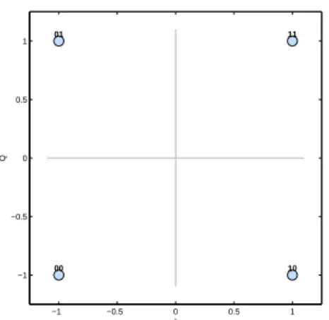
Constellation are a graphical representation of a modulation type. They can illustrate incoherence, noise and Doppler effects that might have affeced the transmission, section 2.6 covers these properties. But a constellation diagram is usually a representation of how data is encoded [20]. The X and Y axes represent two orthogonal entities that are used to encode data into a waveform. Usually X and Y represent the amplitude of the sine and cosine components of an incoming signal, but can also represent two different frequencies, as is the case with FSK. The diagram can also be interpreted as a diagram with polar coordinates, where the distance from the origin is the signals amplitude and the angle is the phase difference between the signal and the carrier.

Every diagram consists of two or more points, as Figure 2.2 illustrates, called symbols, and each symbol corresponds to a pattern of bits. This is used by the modulator to determine which values that should be used on a data stream. The demodulator also uses the diagram to match the symbols of the incoming signal in order to demodulate them back into bits.

2.6 Channel effects

A received signal never looks the same as the transmitted one. Noise have been introduced, Doppler shift have compressed or elongated the waveform, the signal strength have decreased and echoes have been mixed in. These

(14)

−1 −0.5 0 0.5 1 −1 −0.5 0 0.5 1 00 01 10 11 I Q

Figure 2.2: Constellation diagram of QPSK modulation

effects, which complicates the reception, can be seen on the waveform itself or in a constellation diagram [19].

2.6.1 Effect of noise

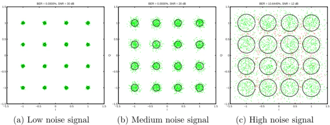
When a signal is demodulated and displayed as a constellation diagram, it will not look the same compared to the original diagram. The points will be scattered which, in turn, can lead to bit errors. Figure 2.3 demonstrates this as each received symbol is mapped into the diagram. Green dots are correctly decoded symbols and red are not. The circles denote the spread of each symbol by the standard deviation.

Figure 2.3a is an example of a signal that can be decoded correctly and

symbols does not interfere with each other. It would be possible to increase the modulation complexity to increase the transfer rate or lower the trans-mission strength in order to save power. Figure 2.3b are not effected by the noise too much, the symbols are still clearly separated and the message can be decoded correctly. Increasing the modulation complexity is not rec-ommended as the noise is to high for more complex modulation types, but lowering the complexity is not necessary either. The same can not be said forFigure 2.3c. The symbols has spread so far that they interfere with their neighbors, causing bit errors. The modulation type is too complex for the current noise level and the complexity should be lowered or the transmission strength needs to be increased.

Different modulation types has therefore different tolerance to noise. Com-plex modulation, 64 - QAM for example, makes the distance between the symbols smaller and therefore makes it more susceptible to noise. The con-verse is also true however. Modulations with low complexity, PSK for

(15)

ex-−1.5 −1 −0.5 0 0.5 1 1.5 −1.5 −1 −0.5 0 0.5 1 1.5 I Q BER = 0.0000%, SNR = 30 dB

(a) Low noise signal

−1.5 −1 −0.5 0 0.5 1 1.5 −1.5 −1 −0.5 0 0.5 1 1.5 I Q BER = 0.0000%, SNR = 20 dB

(b) Medium noise signal

−1.5 −1 −0.5 0 0.5 1 1.5 −1.5 −1 −0.5 0 0.5 1 1.5 I Q BER = 10.6445%, SNR = 12 dB

(c) High noise signal

Figure 2.3: Three diagrams subject to different noise levels.

ample, have larger distances between the symbols and can there for handle noisier environments. These bit errors can be reduced by smart placement of the symbols. A common technique is to restrict two neighbors to only differ in one bit, this is known as Gray Coding.

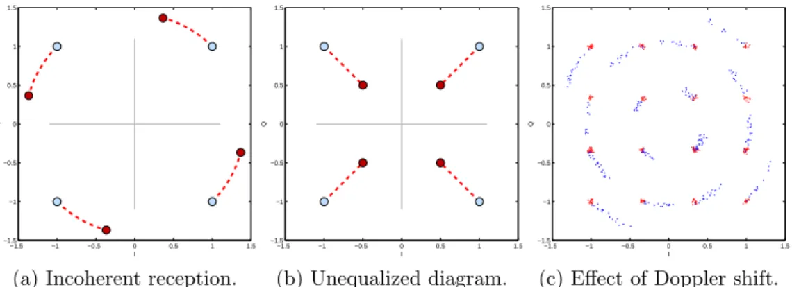
2.6.2 Coherent vs non-coherent

When an incoming coherent transmission is not synchronized the constel-lation diagram will appear rotated. Figure 2.4a illustrates an incoherent reception, the red points are the received symbols and the blue are were

those should be, the diagram is rotated 30◦. Some modulation types require

that the transmitter and the receiver are coherent i.e. have the same phase, others do not.

ASK and FSK are a non-coherent modulation types. They do not require that the phase is correct since they do not have any information encoded in the phase, ASK only checks the amplitude and FSK checks frequency.

PSK is a coherent modulation type. If the transmitter and receiver have

their carriers at more than ±90◦ from each other some symbol will be

in-terpreted wrong. QPSK and QAM are also even more coherent as a even smaller phase offset will cause bit errors.

Some variants of PSK, QPSK and QAM attempts to solve this problem by encoding ones as phase changes and zeros as no changes [18, 24]. The receiver now do not need be coherent as the absolute phase of the incoming signal has no information, only the phase change do. These non-coherent variants are however more susceptible to noise then the coherent ones, but they can simplify the hardware.

(16)

−1.5 −1 −0.5 0 0.5 1 1.5 −1.5 −1 −0.5 0 0.5 1 1.5 I Q

(a) Incoherent reception.

−1.5 −1 −0.5 0 0.5 1 1.5 −1.5 −1 −0.5 0 0.5 1 1.5 I Q (b) Unequalized diagram. −1.5 −1 −0.5 0 0.5 1 1.5 −1.5 −1 −0.5 0 0.5 1 1.5 I Q

(c) Effect of Doppler shift.

Figure 2.4: Two diagram subject to different noise levels.

2.6.3 Signal strength and Doppler effect

The strength of the signal appears as a scaling factor to the diagram. A symbol at (1, 1) can, for example, be found at (5.3, 5.3) or (0.1, 0.1), as Figure

2.4b illustrates. The spread due to noise does not scale however. A symbol

will spread out just as much regardless of the signal strength. Figure 2.3a has therefore a stronger signal compared to the noise than Figure 2.3c, which becomes apparent when the diagram is correctly scaled.

The effect of Doppler causes the symbols to fan out, as Figure 2.4c demon-strates. The blue points are being affected by a very small Doppler shift whilst the red points are not. This is similar to incoherence but instead of being rotated once, the diagram is rotated after every symbol, causing problems with long messages.

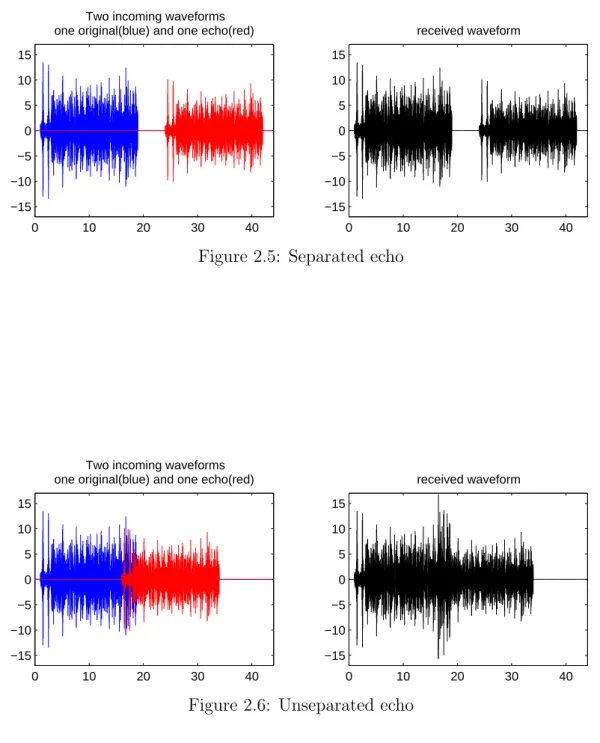
2.6.4 Echoes

One problem for almost all wireless communication is echoes. This occurs especially in indoor and urban areas or in the case of underwater commu-nication, shallow waters and harbors. The echoes can be classified into two categories, separated echoes and unseparated echoes, as illustrated by Figure

2.5 and Figure 2.6 respectively.

Separated echoes are easy to deal with. The fact that they are separated causes the receiver to receive the same message twice. This is no problem as most message contains a serial number and when the same serial number appear twice then the second one can be discarded.

Unseparated echoes are harder to deal with as the two waveforms are colliding and blends together. There are basically two ways to combat this: compensate for the echo or keep the messages short. Echo compensation can

(17)

0 10 20 30 40 −15 −10 −5 0 5 10 15

Two incoming waveforms one original(blue) and one echo(red)

0 10 20 30 40 −15 −10 −5 0 5 10 15 received waveform

Figure 2.5: Separated echo

0 10 20 30 40 −15 −10 −5 0 5 10 15

Two incoming waveforms one original(blue) and one echo(red)

0 10 20 30 40 −15 −10 −5 0 5 10 15 received waveform

(18)

be done by probing the channel, sending out known data, and then create a filter that can remove the echoes. Short message relies on statistics to combat echoes as a short message are less likely to collide than a longer one. This makes most of the echoes into separated echoes.

2.7 Modulation

2.7.1 Why modulate

The purpose of modulation can be illustrated with a radio broadcast station. The producers want to broadcast their radio program to the audience. The information is an analog signal, voice or music, containing frequencies from about 10 Hz to about 10 kHz. To transmit this signal as is, they need an extremely large antenna, several hundred kilometers.

This is not feasible for obvious reasons. Instead they modulate the sig-nal by taking a higher frequency, called carrier frequency, and changing its amplitude to match. The receiver detects the amplitude of the modulated signal and reproduces the original, low frequency, signal.

By modulating it is also possible to add more channels, one station can use its own frequency and leave the rest of the frequency band to others. There are several ways to modulate data, each has its own advantages and disadvantages. Every modulated signal can be written in a polar form:

signal = A sin(2πtF + ϕ) (2.1)

where A is the signal amplitude, t is time, F is the frequency and ϕ is the phase of the signal. A, F and ϕ can be independently varied to modulate data. Equation 2.1 can also be written in Cartesian format:

signal = B sin(2πtF ) + C cos(2πtF ) (2.2)

where B and C determines the signal amplitude and phase.

2.7.2 Digital modulation

Digital modulation uses a carrier frequency to send a few bits a the time. This is a more robust way to transmit information due to the fact that the demodulator receives larger changes in the signal amplitude or phase com-pared to analog information. There are several type of modulation [18] and a few of them are described below. Every type is illustrated by a waveform and a constellation diagram.

(19)

Amplitude shift-keying (ASK) This modulation technique is probably

the simplest example of digital modulations and is a technique used for transmitting one bit at the time. The bit changes the signal amplitude between two values.

0 2 4 6 8 10 12 14 16 0 0.5 1 0x1 0x0 0x1 0x1 0x0 0x0 0x0 0x0 0x1 0x1 0x1 0x1 0x0 0x0 0x0 0x0 data 0 2 4 6 8 10 12 14 16 −1 0 1

Waveform modulated with Amplitude Shift Keying

(a) Modulated Waveform

−1 −0.5 0 0.5 1 −1 −0.5 0 0.5 1 0 1 I Q (b) Constellation diagram

Figure 2.7: ASK modulation

On-off-keying (OOK) There is another variant of ASK and that is to

sim-ply turn the signal on when there is a logical one and off when there is a logical zero. This simplifies the hardware ever further but causes problem when the information consists of many zeros.

Waveform modulated with On−Off Keying

−1 −0.5 0 0.5 1 −1 −0.5 0 0.5 1 0 1 I Q (b) Constellation diagram

Figure 2.8: OOK modulation

Frequency shift-keying (FSK) The information is sent one bit at the

time and the bit determines on which of two frequency too transmit. This technique can be viewed as two OOK on two carriers. The con-stellation diagram is interpreted a little different, the X and Y axis are now not sine and cosine components but two different frequencies.

(20)

0 2 4 6 8 10 12 14 16 0 0.5 1 0x1 0x0 0x1 0x1 0x0 0x0 0x0 0x0 0x1 0x1 0x1 0x1 0x0 0x0 0x0 0x0 data 0 2 4 6 8 10 12 14 16 −1 0 1 Q − sin(2 π f₂ t) 0 2 4 6 8 10 12 14 16 −1 0 1 I − sin(2 π f 1 t) 0 2 4 6 8 10 12 14 16 −1 0 1

Waveform modulated with Frequency Shift Keying

−1 −0.5 0 0.5 1 −1 −0.5 0 0.5 1 0 1 I Q (b) Constellation diagram Figure 2.9: FSK modulation

Phase shift-keying (PSK) Can be viewed as ASK where the amplitude

levels are set to +A and −A. The signal does not vary the absolute

amplitude and has therefore high immunity to signal strength. It is also confined to one frequency, compared to FSK.

Waveform modulated with Phase Shift Keying

−1 −0.5 0 0.5 1 −1 −0.5 0 0.5 1 0 1 I Q (b) Constellation diagram Figure 2.10: PSK modulation

Quadrature phase shift-keying (QPSK) Very similar to PSK but it uses

four phases instead of two. QPSK can be viewed as two PSK, one shifted 90 compared to the other

(21)

0 2 4 6 8 10 12 14 16 0 0.5 1 0x1 0x2 0x3 0x1 0x2 0x0 0x2 0x2 0x3 0x1 0x3 0x1 0x0 0x0 0x0 0x0 data 0 2 4 6 8 10 12 14 16 −1 0 1 Q − cos(2 π f t) 0 2 4 6 8 10 12 14 16 −1 0 1 I − sin(2 π f t) 0 2 4 6 8 10 12 14 16 −1 0 1

Waveform modulated with Quadrature Phase Shift Keying

−1 −0.5 0 0.5 1 −1 −0.5 0 0.5 1 00 01 10 11 I Q (b) Constellation diagram Figure 2.11: QPSK modulation

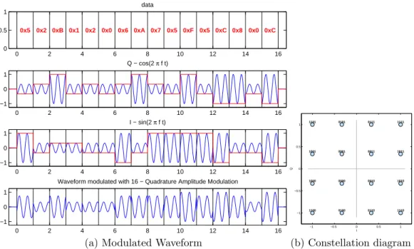
Quadrature amplitude modulation (QAM) is an advanced type of

dig-ital modulation. It uses both the phase and the amplitude to transmit it data. The signal can be expressed as: QAM modulation is often denoted as M-QAM were M is equal to the number of symbols used by the QAM. Higher M-number indicates more bits per symbol but it also means lower resistance to noise.

(22)

0 2 4 6 8 10 12 14 16 0 0.5 1 0x5 0x2 0xB 0x1 0x2 0x0 0x6 0xA 0x7 0x5 0xF 0x5 0xC 0x8 0x0 0xC data 0 2 4 6 8 10 12 14 16 −1 0 1 Q − cos(2 π f t) 0 2 4 6 8 10 12 14 16 −1 0 1 I − sin(2 π f t) 0 2 4 6 8 10 12 14 16 −1 0 1

Waveform modulated with 16 − Quadrature Amplitude Modulation

−1 −0.5 0 0.5 1 −1 −0.5 0 0.5 1 0000 0001 0010 0011 0100 0101 0110 0111 1000 1001 1010 1011 1100 1101 1110 1111 I Q (b) Constellation diagram

Figure 2.12: 16 QAM modulation

Constellation diagrams for QAM need not be square, a circular place-ment of the points are actually more efficient then a rectangular one but is often harder to modulate and demodulate [10].

There are many other types of modulation and variants on the ones stated above. QPSK is an extension of PSK and it can be extend even further by using a 8-PSK, where there are eight symbols instead of two or four. Examples of other types of digital modulation technique include:

• MFSK — Multiple Frequency Shift-Keying

• M-ASK — 4 - Amplitude Shift-Keying, 8 - Amplitude Shift-Keying • DQPSK — Differential Quadrature Phase Shift-Keying

• OQPSK — Offset Quadrature Phase Shift-Keying • MSK — Minimum Shift-Keying

• GMSK — Gaussian Minimum Shift-Keying

(23)

2.7.3 Benefits and drawbacks

The mentioned modulation types have different characteristics as well as strengths and weaknesses. ASK is, for example, not good to use in systems with moving nodes. The signal strength can often vary from place to place and the receiver can wrongly interpret these changes as data. This is also true for OOK.

FSK might be favorable in these situations as the signal strength in not that important, as long as it is stronger than the noise. FSK does however occupy two frequencies, which halves the number of channels that can be utilized.

The phase modulations, PSK, and QPSK, are insensitive to signal strength and does not occupy two frequencies. As a consequence they are often used in digital communication. But these two require coherent carriers, in other words the transmitter and the receiver need to synchronize the phase of the carriers or the data will not be demodulated correctly.

The simpler modulation types, ASK, FSK and PSK, are often used in less expensive digital communication systems [18] as they are easy to implement and they can work in very noisy environments. But simple modulation types mean that the data rate will be low. QPSK and QAM are more complex types capable of higher data rates. QAM inherits the traits of both ASK and PSK as it has problems with both coherency and signal strength.

With more complex modulation, such as QPSK and QAM, comes higher data rate but it also reduces the noise tolerance. These facts will have an impact on the type of modulation chosen for a particular environment. Adap-tive schemes can be used to increase performance of the system, balancing the system between noise sensitivity and data rate.

With these properties in mind, what does it mean for underwater commu-nication? Communicating between two moving vessels could cause problems with ASK and OOK if the messages are long enough. Shorter messages give the channel less time to change and thereby reducing the changes in signal strength during the duration of the transmission.

Moving environments also causes trouble through the Doppler Effect which can shift the frequency outside band used to transmit and receive. This can be more problematic than radio or Wi-Fi as the vehicle velocities relative to the propagation rate is much greater. Two fast ships, closing

at 40 knots each, would cause the frequencies to shift ±2.75% compared to

±0.0075% caused by two Saturn V rockets moving at 11.2 km/s.

These large frequency shifts causes limitations on the system and espe-cially on multi-carrier systems. The carriers need to be separated far enough to accommodate this shift or the speed of the vessels needs to be restricted.

(24)

Compensation for Doppler shift, multi path interference can be done but the time varying nature of the channel can make it a challenge.

2.8 Demodulation

Modulating a signal is of no use if it cannot be demodulated. There are many ways to demodulate a signal, simple modulation types like ASK and FSK only need the presence, or absence , of a signal to demodulate it which can be done by a simple detector. A more general demodulator uses trigonometric identities to process the signal.

Every modulated signal is a sine wave with a certain amplitude, frequency and phase, as stated in equation 2.1 from were the signal can be demodulated. The demodulation is done by multiplying the signal with a sine and cosine wave. When a sine wave is multiplied by an other sine wave with the same frequency produces a raised cosine wave with double the frequency, as shown by the formula for multiplying two sine waves:

sin(θ)· sin(ϕ) = cos(θ− ϕ) − cos(θ + ϕ)

2 and setting ϕ = θ:

sin(θ)· sin(θ) = cos(0)− cos(2θ)

2 =

1− cos(2θ)

2

Calculating the mean value over one period causes the cosine wave to fall away, leaving only a constant.

1 2π ∫ 2π 0 sin(θ)· sin(θ) · dθ = 1 2π ∫ 2π 0 1− cos(2θ) 2 · dθ = 1 2 (2.3)

This constant is also multiplied by the signal amplitude and therefore isolates the amplitude of the sine wave. This is also true for multiplying two cosine waves.

cos(θ)· cos(ϕ) = cos(θ− ϕ) + cos(θ + ϕ)

2

cos(θ)· cos(θ) = 1 + cos(2θ)

2 1 2π ∫ 2π 0 cos(θ)· cos(θ) · dθ = 1 2π ∫ 2π 0 1 + cos(2θ) 2 · dθ = 1 2 (2.4)

(25)

But when doing the same process with a sine wave and a cosine wave the result is zero. Proving the orthogonality between the sine and cosine waves.

sin(θ)· cos(ϕ) = sin(θ− ϕ) + sin(θ + ϕ)

2

sin(θ)· cos(θ) = sin(2θ)

2 1 2π ∫ 2π 0 sin(θ)· cos(θ) · dθ = 1 2π ∫ 2π 0 sin(2θ) 2 · dθ = 0 (2.5)

These three equations, equation 2.3, equation 2.4 and equation 2.5 , makes it possible to isolate the amplitude of the sine and cosine components of a signal.

1 2π

∫ 2π

0

(B sin(θ) + C cos(θ))· sin(θ)dθ =

B 2π (∫ 2π 0 sin(θ)· sin(θ) · dθ ) + C 2π (∫ 2π 0 cos(θ)· sin(θ) · dθ ) = (2.6) B 2 (2.7) 1 2π ∫ 2π 0

(B sin(θ) + C cos(θ))· cos(θ)dθ =

B 2π (∫ 2π 0 sin(θ)· cos(θ) · dθ ) + C 2π (∫ 2π 0 cos(θ)· cos(θ) · dθ ) = (2.8) C 2 (2.9)

The values of B and C can then be mapped to a point in a constella-tion diagram and be reconstructed as one or several bits depending on the

modulation type. In a real system ϕ ≈ θ which reduces the orthogonality

between the sine and cosine waves. Small differences will however have lit-tle effect on a good demodulator and large differences should be dealt with before demodulation.

(26)

1.2 1.4 1.6 1.8 2 2.2 2.4 x 104 −60 −50 −40 −30 −20 −10 0 frequency (Hz) signal strength (dB) frequency spectrum 1.2 1.4 1.6 1.8 2 2.2 2.4 x 104 −60 −50 −40 −30 −20 −10 0 frequency (Hz) signal strength (dB)

simplified frequency spectrum

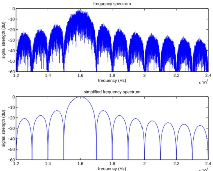
Figure 2.13: 16 kHz carrier modulated with 1 kilo symbols per second

2.9 Orthogonal frequency division

multiplexing

OFDM is a technique used by multi carrier modulators and as a multiple access technique [9]. In OFDM several frequencies chosen such that they do not interfere with each other, as the word orthogonal implies.

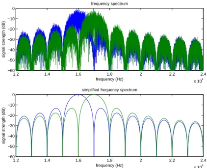
When a carrier is modulated with a digital modulator it spreads out in frequency. The characteristics of the spread will depend on the symbol rate. The frequency spectrum of a simulated modulation with random data shown in Figure 2.13 demonstrates a 16 kHz carrier modulated with QPSK at 1000 symbols per second. Notice the large ”hump” centered at 16 kHz, but more interesting are the ”ravines” at 14, 15, 17 and 18 kHz.

These ”ravines” are located at 16± N kHz. This is due to the fact that

the signal is modulated at 1000 symbols per second. If the same carrier was modulated at 2000 symbols per second the ”ravines” will be located at

16±2N kHz. These ”ravines” can be exploited. If another carrier is added at

a ”ravine”-frequency it would not be subject to interference form, or interfere with, the first carrier. Figure 2.14 show that this is true. Note that none of the two interfere at 14, 15, 18, 19 and 20 kHz, these can therefore be used for even more carriers, as Figure 2.15 illustrates.

(27)

Figure 2.14: 16 and 17 kHz carriers modulated with 1 kilo symbols per second

Figure 2.15: Five carrier frequencies spaced at 1 kHz apart, each modulated with 1 kilo symbols per second

(28)

This can also be shown mathematically. Equations 2.3, 2.4 and 2.5 can be modified to account for two different frequencies that both are integer multiplications of a common frequency.

1 2π ∫ 2π 0 sin(M θ)· sin(Nθ) · dθ = 1 2π ∫ 2π 0 cos(θ(M − N)) 2 · dθ (2.10) 1 2π ∫ 2π 0 sin(M θ)· cos(Nθ) · dθ = 1 2π ∫ 2π 0 sin(θ(M − N)) 2 · dθ (2.11) 1 2π ∫ 2π 0 cos(M θ)· cos(Nθ) · dθ = 1 2π ∫ 2π 0 cos(θ(M − N)) 2 · dθ (2.12)

Where M and N are natural numbers greater than zero. If M = N then: 1 2π ∫ 2π 0 cos(θ(M − N)) 2 · dθ = 1 2π ∫ 2π 0 1 2· dθ = 1 2 1 2π ∫ 2π 0 sin(θ(M − N)) 2 · dθ = 1 2π ∫ 2π 0 0· dθ = 0

which is already proven in section 2.8, but if M ̸= N then the integrals will

evaluate to zero as:

∫ 2π 0 cos(θX)· dθ = 0 ∫ 2π 0 sin(θX)· dθ = 0

Where X are a non-zero integer. Therefore any set of two frequencies that are a integer multiple of a common frequency are orthogonal to each other. Which is the fundamental theory behind the Fourier transform.

2.10 Error correcting and interleaving

There are many ways to ensure that a received message has been received correctly. The easiest way is to implement some type of checksum. A parity bit could be inserted to ensure that the number of ones in the bit stream are even, if the receiver message do not have a even amount of ones then the message is incorrect. This can then only detect odd number of bit errors, if two bits are wrong then the message will still contain an even number of ones.

A slightly more sophisticated way is to add a checksum ensuring that the unsigned sum of every byte in the message are zero. This can detect several

(29)

d1 d2 d3 d4 d5 d6 d7 d8 d9 d10 d11

p1 p2 p3 p4 p

Figure 2.16: Hamming code with four error correcting bits and one global parity bit, denoted as Hamming(16,11)

errors in the same message. There are also cyclic redundancy check s that can find many errors and are also guarantied to find every odd number of bit errors.

All these types have one drawback, they can detect errors but they can not correct them. There are some types of coding, called error correcting code or Forward Error Correcting (FEC) code. These methods add redundant information into the message making it possible to correct the errors when the message is received.

The simplest type of FEC is what is called repetition code [26], where every bit is repeated an even number of times. The receiver uses the most common value of these bits to correct the message. If every bit is repeated two times and the receiver receives 110 then it is more likely that the real sequence should have been 111 than 000, the receiver therefore classifies this as a 1. If the system uses five bits instead of three than two bit in every five-bit block can be wrong without impacting the actual message, but the transmission is now five times as long.

In 1950 Richard Hamming published what is now know as the Hamming code which takes the concept of parity bits one step further [4, 21]. He implemented a system where several parity bits worked together to identify where in a message an error is, he could then correct it. Hamming code has much less overhead than repetition code and the relative overhead decreases as the block size increases. However it can only correct a single bit in a block, which becomes a problem when using large block sizes.

Hamming code are denoted Hamming(A,B), were A is the length of the block and B is the number of information bits. Hamming(7,4) is four data bits converted into seven bits, illustrated by Figure 2.16. Hamming code are often implemented together with an additional parity bit making the code able to correct one error in every block and but detect two errors, this is what is known as Single Error Correction, Double Error Detection or SECDED.

There are also several more types of FEC that all have different properties. There are Reed-Solomon code, turbo code and many others. Most types of FEC are good at correcting a few errors located randomly across the message, few, if any, are good a combating error bursts where several bits are wrong in a small part of the message. There are however a way to combat this, not by tackling the problem head on but to reduce the problem.

(30)

Message Interleaved message with errors Interleaved message Message with errors Deinterleaved message

Figure 2.17: An example of interleaving

This is where an interleaver steps in. An interleaver is a device that takes a long message and shuffles the bit around before they are transmitted. After reception a deinterleaver shuffles them back into the correct order. If a mes-sage contained burst errors these will now be spread out by the deinterleaver, as shown in Figure 2.17, and the FEC can now correct the blocks that now contains fewer bit errors per block, making it easier to correct.

(31)

Chapter 3 Implementation

3.1 Physical layer structure

The structure of the physical layer for an acoustic underwater modem are shown in Figure 3.1. Some of these layers are necessary to be able to trans-mit and receive and others are not. The order of the layers can in some cases be interchanged but the structure shown is recommended. The layer required for a minimalistic system are Modulation, Demodulation and De-tection. With these three layers implemented the system can modulate a data stream, detect the transmitted waveform and demodulate it. However being a minimalistic system it will not limit the frequency bandwidth, not tolerate any movement and require a strong signal.

Adding layers can fix those problems. A filter just before transmission can remove the frequencies outside the bandwidth assigned to the channel and constant tones, or pilot tones, can be added to the signal. These will be used for Doppler compensation [12] after a incoming waveform has be detected.

The topmost layers, compression and decompression, is an example of a layer that is not necessary. But being able to compress the message reduces collision probability, transmission time and thereby saves power. Encryption and decryption are also not necessary but can protect data from compet-ing companies or enemies. Error correction, interleavcompet-ing and deinterleavcompet-ing are not necessary either although they enable the system to work in noisier environments.

The physical layer is implemented in four steps. The first step is to choose the type of modulator and demodulator, read more in section 2.7. Secondly an envelope detector are necessary in order to locate where in the incoming

(32)

Physical

Interleaving Error Correcing Modulation

layer

Deinterleaving Error Correcing Demodulation Doppler correction

Physical

layer

Encryption Compression Decryption Decompression Pilot signals

Bandwidth limiting Detection

Figure 3.1: Structure of physical layer in an acoustic underwater modem.

stream of samples a message might be. The type of detector is dependent on the type of modulator used and the expected length of the messages.

These two steps are sufficient and necessary in order to make a transmis-sion and receive it. But it will vulnerable to noise and other sources that can cause bit errors. Therefore, the third step is to choose a type of error correction. The type of environment will determine the type chosen as more robust coding might be needed in shallow waters compared to deep water due to the complex multi-path phenomenons. The type of interleaver should also be chosen together with the FEC as some types of FEC perform bet-ter with a matching inbet-terleaver [15]. A filbet-ter often needs to be added before transmission to restrict the signal to the frequency range used by the system. The fourth, and last step, concerns the non-essential components such as Doppler compensation and encryption. Are those needed or not. Encryption and compression could be left to the application to implement if so needed. Doppler compensation should always be placed in the physical layer if it is used.

(33)

Parameter Value Unit Frequency band 16− 32 kHz Maximum range 1 km 0.54 nautical miles Sampling frequency 100 kHz Maximum depth 60 m 200 feet

Transmission strength 185 dB relative 1µPa @ 1 m

Maximum speed of receiver 8 knots

4.115 m/s

Maximum speed of transmitter 8 knots

4.115 m/s

Table 3.1: Table of technical specifications.

3.2 Structure of the implementation

To be able to complete the steps described in the previous section an under-standing of the system requirements is required. The specifications used for the implementation are mentioned in Table 3.1. Some of the parameters are fabricated and others are similar to other systems.

A multi carrier structure was chosen as the available bandwidth can then be subdivided into smaller subcarriers. These can then be used independently or collectively to transmit and receive the data. The primarily reason was to reduce the message length by transmitting on multiple carriers at once. Further more was a OFDM structure chosen, with symbol rate of 1000 symbol per second, as the frequencies are orthogonal and therefore does not disturb each other.

An early idea was to include a start and a key symbol at the start of the transmission. The start symbol or pilot symbol [9] is often used to sense incoming messages and to equalize the symbols. The key is used to identify the type of modulation used on the respective channels. With the key it is possible to actively change the modulation type to fully utilize the channel [7].

The structure of the chosen envelope detector are a simple amplitude change detector. The current signal amplitude are compared to the amplitude from x samples ago and a message are detected by a rise in the strength by a factor of y. The end is detected similarly by the fall of the signal strength. A Doppler compensation module is not implemented, neither is encryp-tion nor compression. The network [1] is assumed to be a staencryp-tionary network

(34)

Physical

Interleaving Error Correcing Modulation

layer

Deinterleaving Error Correcing Demodulation

Physical

layer

Detection Simulator

Figure 3.2: The structure of physical layer of the implementation.

through which sensors can relay information to a data central. The Doppler effect will then have limited influence and there is no need for encryption or compression. Error correction is however something that will be needed. A Hamming code was chosen for this purpose and complimented with a inter-leaver to increase its efficiency.

Lastly a simulator replaces the hardware layer in order to be able to test the algorithms. With these choices made the structure of the physi-cal layer changed from Figure 3.1. Compression/Decompression, Encryp-tion/Decryption, Pilot signals/Doppler correction and Bandwidth limiting are layers that have disappeared reducing the physical layer to Figure 3.2.

The following sections will describe the implemented layers. Section

3.4 covers the modulation and demodulation layers. The detector-, error

correcting- and interleaver layers are covered in section 3.3, section 3.6 and

section 3.7 respectively. Section 3.8 covers the principle of a publish

sub-scribe architecture on which the system could be implemented.

3.3 Envelope detector

The objective of an envelope detector is to figure out were in a sample stream a message might be located. It should be able to find the start of a message as well as the end, store the waveform from beginning to end a then hand it over to the demodulator for further refinement. It must also be tuned to match the modulator as the type of modulator will determine the complexity of the envelope detector.

(35)

The implemented envelope detector first filters the incoming waveform to eliminate all frequencies not part of the frequency band and then uses a similar process as a first stage. It uses the absolute value of each sample instead of the sample value itself. This enables the detector to find peaks regardless of whether it is positive or negative. This is expressed in equation

3.1.

envelopen= max (envelopen−1· α, |samplen|) (3.1)

were the value of α determines the leakage. Smaller α results in a faster

decent back to zero. The value of envelopenis then compared with the value

from many samples ago and then filtered with a simple first order filter.

detectorn= detectorn−1· β + min

( envelopen envelopen−M , γ ) · (β − 1) (3.2)

were M determines how far back to compare the values, γ is a very small number to prevent division by zero and β controls the rise time of the filter. This value is then compared with a threshold value to determine if the change in signal strength was strong enough.

f oundn= detectorn> B (3.3)

When the detector has detected a waveform it start recording the waveform. However, the interesting waveform actually started a while ago since it took time for the detector value to reach the threshold value and this must be compensated for. One solution is to mark a previous value as the starting point as well, as demonstrated by equation 3.4.

f oundn−S = f oundn−S∨ foundn (3.4)

The values of α, β, γ, M and B are adjusted according the to settings on the modulator and the properties of the channel.

Figure 3.3 demonstrates this process. The blue curve are the incoming,

filtered signal, the green are the envelope variable, the red are the detector value and the cyan are the found variable. The entire waveform marked by the found variable will be transmitted to the demodulator for demodulation. The envelope detector also marks an interval where the start is located. This is based on the position of the start symbol within the waveform.

(36)

745 750 755 760 765 770 775 780 −50 −40 −30 −20 −10 0 10 20 30 40 50 waveform envelope detector found

(37)

Modulator 30 kHz Modulator 31 kHz Modulator 29 kHz Modulator 28 kHz Modulator 27 kHz Modulator 26 kHz Modulator 25 kHz Modulator 24 kHz Modulator 23 kHz Modulator 22 kHz Modulator 21 kHz Modulator 20 kHz Modulator 19 kHz Modulator 18 kHz Modulator 17 kHz OFDM modulator

Figure 3.4: OFDM modulator structure

3.4 Modulator and demodulator

implementation

The implemented structure of the modulator is an OFDM structure, shown in Figure 3.4. The OFDM modulator consists of several internal modula-tors, each responsible for a individual frequency, and a set of constellation diagrams. The submodulators can be set individually to different modulation types, from turned off to 64 QAM. They can also be used for constant tones, known as pilot tones, that is used to correct Doppler shifts.

The OFDM transmits on every modulator at once and synchronously. A transmission start with all the submodulators sending their start symbol and key symbol as a type of header and following the header is the payload data. The header is used by the receiver for synchronization proposes.

The structure of the OFDM demodulator is similar to the modulator. It also consists of several internal demodulators and the same set of constella-tion diagrams. To be able to demodulate a message the OFDM demodulator needs a waveform containing the entire message and an interval of were the start is located. The demodulation process then follows a specific proce-dure to find exactly were the start is, which channels are used, what kind of modulations is used and the length of the message.

3.4.1 Processing incoming waveform

The first step is to loop over the starting interval. For every iteration the demodulators are set to assume that the current position is the start of the message. From this assumed start the demodulators extracts the symbols of the message. The symbols are most certainly not correctly aligned with the constellation diagrams due to incoherency and signal strength mentioned in

(38)

A θ

Figure 3.5: Symbol equalization

matrix. The matrix is constructed such that the first symbol is placed exactly in the correct position. The rest of the symbols are then equalized using the same matrix. M = A [ cos(θ) sin(θ) − sin(θ) cos(θ) ] = [ A· cos(θ) A · sin(θ)

−A · sin(θ) A · cos(θ)

]

(3.5) where A is the scaling factor and θ is the rotation, also shown in Figure 3.5.

A and θ is calculated such that: M [ Xstart Ystart ] = [ 1 1 ] .

The values are calculated by matrix inversion and result in the following equations:

A cos(θ) = Xstart+ Ystart

X2

start+ Ystart2

(3.6)

A sin(θ) = Ystart− Xstart

X2

start+ Ystart2

(3.7) If the assumed start was the real start, or close to the real start, the rest of the symbols will start to be clustered by their respective symbol in the diagram. The demodulator now measures how much each diagram symbol has been spread out and correlates the placement of the second symbol, the key symbol.

(39)

This measurement value is called a fitness value and is calculated for every modulation type. This is done by summing up the square of the distance between each incoming symbol and the closest symbol in the diagram. The fitness value is then penalized if the key is located too far from its correct position. Taking the logarithm of the measurements compensates for the difference in noise levels on the different channels.

The final fitness value is the set to the value of the best fitting modulation type. This process can be summarized by the following expression:

f itness = max

j (− log[errorkeyj ·

n

∑

i

∥symboli− closestj,i∥2]) (3.8)

were i is every symbol in the waveform and j is every modulation type. The gain of the equalization matrix, the value of A in equation 3.5, is also measured, by taking the logarithm of the determinant of the matrix:

gain = log(det(M )). (3.9)

With these values for every iteration and every channel, the demodulator can determine the correct start of the message and which channels are being used.

The demodulator starts a second iteration. Firstly, for every iteration the gain values are normalized. The normalization adjusts the values linearly such that the lowest value is normalized to zero and the largest to one. Then a cluster analysis is performed with two clusters, starting at 0 and 1. The idea being that an unused channel will cause the gain value to be significantly larger than the rest as the matrix tries to make sense of the noise. The clusters are compared and the difference between them, the separation

strength is measured.

If the greatest separation strength, of all iterations, is larger than a thresh-old value there are most likely some channels that are not in use. Empirical experiment performed during development show that the normalized gain values for a used channel is often less than 0.1 and unused channels has values greater than 0.9, if there is any unused channels. A threshold value is therefore chosen to 0.8. If the clusters are clearly separable, the maxi-mum separation strength is greater than 0.8, then the OFDM demodulator starts identifying the channels with an average normalized gain above 0.5 and turning them off, otherwise every channel is assumed to be used.

With the active channels identified, the demodulator summarizes the fit-ness values of every active channel and assumes that the point with the greatest fitness is the start of the message. Each demodulator can now be adjusted to the corresponding modulation types and find the end of the

(40)

message. The system can now proceed with the decoding process. Each demodulator matches each symbol against the diagram and append the cor-responding bit in the same manner as the modulators extracted them. The demodulated bit stream can now be passed on to the next stage for further processing.

3.4.2 Single carrier modulator and demodulator

Figure 3.4 shows that one OFDM modulator consists of several single carrier

modulator, fifteen modulators are used in the figure.

The single carrier modulators are versatile, since they can be used in a multi carrier system, like the OFDM modulator, or on their own. The modulation type can be varied from completely turned off to 64-QAM, this makes the OFDM system able to change the modulation type of each channel according to the noise level on that particular channel.

The modulator is connected to a bit stream from which it can extract the bits it need to create the symbol. If the modulator requests more bits than are available the bit stream will append extra zeros to the symbol. Several modulators can be connected to the same bit stream and request bits one modulator at the time.

As some systems are subject to Doppler effect, the modulator can act as a pilot tone. In this mode the modulator will not request any bits and will instead send a constant tone. The modulator can also be set to modulate a random symbol. This can be used in a Frequency Hopping scheme where it might be needed to disguise the true message by filling the unused frequencies with nonsense information.

The subdemodulators does the same as what the submodulators do but in reverse. They are also responsible for calculating the equalization matrix and compute the fitness values.

3.4.3 Generation of the constellation diagrams

In order to be able to modulate at all several constellation diagrams needs to be generated. The diagrams are generated by three algorithms, two for ASK and PSK and one for QPSK and QAM. The algorithm for the ASK returns the symbol (1, 1) if the bit was a one and (0, 0) if the bit was a zero. Similarly

with PSK but with the coordinates (1, 1) and (−1, −1) respectively.

The QPSK and QAM algorithm is a recursive one. It starts with a point at (1, 1) and reflects the point over one axis if the first bit is zero, and over the other axis if the second is zero. In this way the diagram for QPSK is created. Note that first quadrant of the 16-QAM diagram has the same structure as

(41)

Figure 3.6: Recursive constellation diagram

the QPSK, it has only been moved away from the origin. This is illustrated in Figure 3.6

This is exploited by the algorithm, it moves the point into the first quad-rant, by adding the vector (2, 2). Then the point is reflected again according to the values of the next two bits. This however changed the scale of the di-agram, as points now can appear at (3, 3) for example, but this is corrected as the last part of the algorithm. Now that a 16-QAM diagram has been created the move-and-reflect procedure can be repeated to achieve 64-QAM,

256-QAM, 1024-QAM and any 4N1_-QAM.

This recursive constellation diagram also has the nice property that the symbols are arranged in a gray pattern, were two neighbors only differ in one bit. The reverse algorithm is also recursive. The quadrant of the coordinate first determines the value of the two bits and then the coordinate are reflected into the first quadrant after which the point is moved, ready for the next step. The diagrams can also be generated as look-up-tables which is more effi-cient for the modulator but less effieffi-cient for the demodulator. The modulator need only fetch the correct values from the table but the demodulator must compare every incoming symbol to every entry in the table to find the closest one. This is no problem when using less complex modulation types since the number of comparisons are relatively low, but highly complex modulation types has several hundred symbols. This means if a look-up-table consists of N symbols then N comparisons need to be made, making the the table approach a O(N ) algorithm. The recursive algorithm needs only perform

(42)

the algorithm one step deeper when the symbols increase by a factor of four, making this a O(log N ) algorithm.

3.5 Simulator

The simplest simulator to implement is none at all. Sending a waveform from the modulator directly to the demodulator is a simple way to test if the modulator and demodulator implementations work together. But the real world is full of unknowns that this approach does not model. For example:

Unknown arrival time A waveform can arrive at any time. The

demodu-lator can not, and should not, know when a message should arrive.

Noise A waveform will always suffer to noise of some kind. Noise sources

are everywhere, wind, rain, waves, ship traffic and even mammals, fish and crustaceans.

Echoes The waveform will also suffer from echoes. See section 2.6.4 for

more information.

Doppler effect All moving objects can have an Doppler effect on the signal.

Moving the transmitter or receiver are classical examples but of equal importance are echoes for moving objects.

Accurate simulator needs to account for all these properties and also the fact that these properties change with time. The implemented simulator is much simpler than that, it assumes that the environment is static and that the messages are so short that only separates echoes will reach the receiver.

Therefore it only models the unknown arrival times and the noise. The

implemented simulator is also not a real time simulator, meaning that it does not run simultaneously as the modulator and demodulator.

The simulator works by simply modifying the waveform to something similar to what the receiver might receive and it start by creating empty waveform, much longer than the incoming waveform. Then it places the incoming waveform in a randomly chosen place in the empty waveform. This imitates the unknown arrival time of the underwater channel. The placement if chosen within a interval to make debugging the demodulator easier. Noise is then added to the waveform according to a specified signal-to-noise ratio. This new longer and noisier waveform can then be fed to the demodulator to tune the reception and test its performance.

(43)

Data bits

Hamming parities Global parity

Bits

Figure 3.7: Structure of the Hamming coder

3.6 Error correction

In this implementation Hamming coding is used. The structure of the Ham-ming coder uses a large array of booleans and a data structure that keeps track of what each bit represent. The array is large enough to accommodate most block sizes and can also be trimmed down if memory is very expensive.

Figure 3.7 illustrates the couplings between the pointers and the array.

The system can be defined in two ways: either by specifying the number of data bits that should be used, or by the total length of the block. Regardless of the definition the coder must figure out the number data bits, the number of Hamming parities and the length of the block. Pointer are then allocated and connected according to the definition. Compare Figure 3.7 with Figure

2.16 on page 28.

The encoding process is done by loading the array with the incoming data though the data bit pointers. Then the Hamming parities can be calculated followed by the global parity. The bit array is the converted to a value that can be send to the interleaver. The decoding process work in the opposite direction. A value from the deinterleaver is converted into the bit array and the parities are checked. The block is corrected, if needed, and then sent to the next layer of the system.

3.7 Interleaver

The data structure of the interleaver consists of two array one connected to the other. The way these array are connected is determined by the type of interleaver that is implemented. A matrix interleaver will rearrange the incoming data by working with a matrix, filling it row wise and emptying it

(44)

Array of data pointers

Array of data

Figure 3.8: Matrix interleaver

column wise, as the following shows: [ 1 2 3 4 5 6 7 8 9 ] →   1 2 34 5 6 7 8 9   →[ 1 4 7 2 5 8 3 6 9 ]

The connections for this structure are arranged such that it can reproduce this behavior by writing data in one array and reading through other. This is shown in Figure 3.8, but this interleaver works with blocks of eight rather than nine. Deinterleaving work in the same way but in the opposite direction. There are also a helical scan interleaver that also uses a matrix to interleave the data but the matrix are emptied in a diagonal fashion.

A random interleaver works as the name implies, the connections are are connected in a random fashion, shown in Figure 3.9. This structure is a little more complex to implement. Most random number generators are global, meaning that any part of the program can get a value and by doing so changing the value for the next part trying so acquire a value. This is obviously bad if these values are used to setup the structure of a random interleaver. Therefore the seed for the random number generator must be preset to a predefined value before creating the structure. Or a local random number generator can be used instead of the global one.

The implementation of the interleavers are the same. Every type has the two arrays and the only difference is the way that they are connected. It is therefore practical to implement the interleavers using an abstract class in a object-oriented programming language and using inheritance for the specific types of interleavers. These connections are defined by a skip factor for the matrix interleavers and by a linear feedback shift register for the random interleaver.

(45)

Array of data pointers

Array of data

Figure 3.9: Random interleaver

3.8 Publish and subscribe

Publish and subscribe, or PubSub, is a messaging type used for interprocess communication [8, 25]. The communication process is similar to a person reading magazine. The sender ”publishes” the relevant information in the magazine and any one that is interested in that information can ”subscribe” to the magazine and read it. The receiver is not interested in who published the information and the sender in not interested in who gets it.

This connection, with independent and anonymous behavior, is good for modular software design. One module can be interchanged by another or multiple modules without affecting the rest of the system, this can even be done on-line in some cases. Every message type is what is known as a topic. One process may publish to and subscribe from several topics.

The weakness of such a system is the fact that the modules are so anony-mous and independent. If a module, responsible for error checking, crashes, none in the system are aware of it [25].

Lets say a car has an airbag checking module, it sends messages to the airbag and expects a reply in order to make sure that the airbag are ready to deploy if needed. If it does not receive a reply it will publish on a error topic, letting the system know that the airbag may not be working. If that module should crash there will be no publications made to the error topic and when the airbag eventually stops working no one will be informed. This could obviously have major consequences.

Software defined acoustic underwater modem