A Decision Support System for Stress
Diagnosis using ECG Sensor
Thesis Report By:
Mohd Siblee Islam (860116-9793) Supervised By:
Shahina Begum and Mobyen Uddin Ahmed Examiner:
Professor Peter Funk
School of Innovation, Design and Engineering (IDT) Mälardalen University
i
Abstract
Diagnosis of stress is important because it can cause many diseases e.g., heart disease, headache, migraine, sleep problems, irritability etc. Diagnosis of stress in patients often involves acquisition of biological signals for example heart rate, finger temperature, electrocardiogram (ECG), electromyography signal (EMG), skin conductance signal (SC) etc. followed up by a careful analysis of the acquired signals. The accuracy is totally dependent on the experience of an expert. Again the number of such experts is also very limited. Heart rate is considered as an important parameter in determining stress. It reflects status of the autonomic nervous system (ANS) and thus is very effective in monitoring any imbalance in patient’s stress level. Therefore, a computer-aided system is useful to determine stress level based on various features that can be extracted from a patient’s heart rate signals.
Stress diagnosis using biomedical signals is difficult and since the biomedical signals are too complex to generate any rule an experienced person or expert is needed to determine stress levels. Also, it is not feasible to use all the features that are available or possible to extract from the signal. So, relevant features should be chosen from the extracted features that are capable to diagnose stress. Again, ECG signal is frequently contaminated by outliers produced by the loose conduction of the electrode due to sneezing, itching etcetera that hampers the value of the features.
A Case-Based Reasoning (CBR) System is helpful when it is really hard to formulate rule and the knowledge on the domain is also weak. A CBR system is developed to evaluate how closely it can diagnose stress levels compare to an expert. A study is done to find out mostly used features to reduce the number of features used in the system and in case library. A software prototype is developed that can collect ECG signal from a patient through ECG sensor and calculate Inter Beat Interval (IBI) signal and features from it. Instead of doing manual visual inspection a new way to remove outliers from the IBI signal is also proposed and implemented here.
The case base has been initiated with 22 reference cases classified by an expert. A performance analysis has been done and the result considering how close the system can perform compare to the expert is presented. On the basis of the evaluations an accuracy of 86% is obtained compare to an expert. However, the correctly classified case for stressed group (Sensitivity) was 57% and it is quite important to increase as it is related to the safety issue of health. The reasons of relatively lower sensitivity and possible ways to improve it are also investigated and explained.
iii
List of Figures
Figure 1: CBR cycle [47]. ... 6
Figure 2: Steps of the work ... 11
Figure 3: The Decomposition steps of Daubechies Discrete Wavelet Transformation [40]-[42]. ... 17
Figure 4: Mean values calculation by sliding the window. ... 19
Figure 5: Mean value calculation by considering the highest frequency. ... 20
Figure 6: Proposed algorithm to detect and replace outliers. ... 20
Figure 7: Removal of outlier by replacing it with previously accepted adjacent data points .. 21
Figure 8: Fuzzy Similarity using triangular membership function [34] [35] ... 24
Figure 9: Data Collection by using software prototype ... 26
Figure 10: Online graph of ECG Signal ... 26
Figure 11: Online graph of IBI Signal calculated from ECG Signal ... 27
Figure 12: Calculated frequency domain features ... 27
Figure 13: Original and Filtered (After removing outliers) IBI ... 28
Figure 14: ER Diagram of CBR system ... 29
Figure 15: MVC System Architecture ... 30
Figure 16: The system Diagram ... 30
Figure 17: Expert’s overall classification compared to classification obtain from individual biological Signal ... 32
Figure 18: Probability of a case to be classified as stressed Vs Sensitivity for class libraries for k = 1. ... 38
Figure 19: Probability of a case to be classified as stressed Vs Sensitivity for class libraries for k = 2. ... 38
Figure 20: Probability of a case to be classified as stressed Vs Sensitivity for class libraries for k = 3. ... 38
Figure 21: Sensitivity Vs k value for all case libraries ... 39
Figure 22: Accuracy of the system Vs k value. ... 39
iv
Figure 24: Comparison of sensitivity improvement by increasing of the probability of a case to be classified as stressed and k value. ... 40 Figure 25: The effect on system performance after increasing of the probability of a case to be classified as stressed and k value. ... 41 Figure 26: The effect on specificity after increasing of the probability of a case to be
vi
List of Tables
Table 1: The list of time and frequency domain features ... 12
Table 2: List of the Time Domain features that are used in HRV analysis ... 13
Table 3: List of the Frequency Domain features that are used in HRV analysis ... 13
Table 4: Lists of the Frequency ranges used in HRV analysis ... 14
Table 5: List of the equations that are used for normalizing LF and HF in the HRV analysis 14 Table 6: Features extraction and selection ... 15
Table 7: The list of DWT features [40]-[42]. ... 17
Table 8: Average values of features extracted from ‘good’ sample G, ‘bad sample’ B and ‘repaired sample’ R, for individual S1, S2 and S3 ... 21
Table 9: Distances between ‘good sample’ and ‘bad sample’ based upon the Time Domain features before and after correction ... 22
Table 10: Distances between ‘good sample’ and ‘bad sample’ based upon the Frequency Domain features before and after correction ... 22
Table 11: Distance between ‘good sample’ and ‘bad sample’ based upon all the Features before and after correction ... 22
Table 12: Case representation ... 23
Table 13 : Classification of the cases based on FT, HR and RR individually and based on all three biological signal where 'H' represents 'Healthy' and 'S' represents 'Stressed' ... 31
Table 14: Step of the Weight List ... 32
Table 15: Time Domain Weight List ... 32
Table 16: Frequency Domain Weight List ... 33
Table 17: Frequency Domain Weight List ... 33
Table 18: CBR evaluation for DWT where weight of level 1 = 100%. ... 34
Table 19: CBR evaluation of DWT for each level and combination of various levels. ... 34
Table 20: Various domains and their combinations are represented with correctly classified cases, miss diagnosis of stressed and miss diagnosis of healthy ... 35
Table 21: The description of case libraries that are generated from main library by reducing the cases classified as healthy to increase the probability of a case to be classified as stressed. ... 36
vii
Table 22: Percentage of correctly classified cases, Sensitivity and Specificity for all the case libraries ... 37 Table 23: The accuracy of the system classification, sensitivity and specificity according to the size of the class library. ... 37
ix
List of Abbreviations
ANS Autonomic Nervous Systems CBR Case Based Reasoning DBN Dynamic Bayesian Network DWT Discrete Wavelet Transformation FFT Fast Fourier Transformation FT Finger Temperature HF High Frequency HR Heart Rate
HRV Heart Rate Variability IBI Inter Beat Interval LF Low Frequency MF Medium Frequency
pNN 50 Percentage of NN 50 in total number of beats. PSD Power Spectrum Density
RMSSD Root Mean Squire of the all Successive RR interval difference. RR Respiration Rate
SDNN Standard deviation of NN intervals SNS Sympathetic Nervous System TP Total Power
ULF Ultra Low Frequency
xi
Content
1. Introduction ... 1
1.1 Objective of the Thesis ... 2
1.2 Problem Formulation ... 2
1.3 Solution for the Problem ... 2
2. Background and Related Work ... 5
2.1Background ... 5
2.2 Related Work ... 8
3. Approach and Method ... 11
3.1 IBI Signal and Preprocessing ... 11
3.2 Feature Extraction ... 12
3.3 Feature Selection ... 14
3.4 Data Collection and Prototype Implementation: ... 17
3.5 Preprocessing and Getting IBI ... 18
3.6 Case Representation ... 23
3.7 Similarity Function ... 23
4. Implementation ... 25
4.1 Software Prototype Implementation ... 25
4.2 CBR Implementation ... 28
5. Result and Evaluation ... 31
6. Discussion and Future Work ... 43
7. Summary and Conclusion ... 45
1
1. Introduction
Stress is popularly known as the state when a person fails to react properly to the emotional or physical threats whether imaginary or real. It shows symptoms like exhaustion, headache, adrenaline production, irritation, muscular tension and elevated heart rate. When our brain appraises stress, the Sympathetic Nervous System (SNS) prepares our brain to respond to stress. The beat to beat intervals of the heart tend to vary. This gives rise to Heart Rate variability (HRV) which is mostly regulated by the sympathetic and parasympathetic Autonomic Nervous Systems (ANS) [1]-[6]. Thus the state of the ANS is reflected in HRV. This has made it an increasingly popular tool to investigate the state of the ANS, which can be further used to explain various physiological activities of the body [2], [7]-[8]. Heart rate variability (HRV) is one of the popular parameters to analyze the activities of the Heart and the Autonomic Nervous System (ANS) in humans [2]. The state of the ANS is reflected in the HRV. For this reason we chose HRV as one of the key criteria to diagnose stress.
But the heart rate signal is non-stationary [48] and the signal pattern is also different from person to person [1]. Even the range of the signal depends on the type of population like man, women, infant, animal and the physical condition like healthy or sick. That is why it is really hard to formulate any rule by that the diagnosis of stress is possible. The diagnosis is mainly based on the expert’s experience but the number of expert is also insufficient. In such a scenario a case base reasoning (CBR) system can be considered as a way of stress diagnosis. In CBR the nature of new problem is identified and solved respectively by reusing the previous problems and their solutions that are categorized and solved by expert [47].
The HRV can be analyzed using both time domain and frequency domain attributes. It is very important to choose features which vary with the changes of the stress levels and show relatively reliable behavior. Overall, heart rate variability spectra during baseline conditions are dominated by high frequency activity, a reflection of parasympathetic efferent neuronal innervations and linkage to the ventilatory cycle manifested as respiratory sinus arrhythmia. Stress is accompanied by an increase in the Power Spectrum Density (PSD) of Low Frequency (LF) and decrease in PSD of High Frequency (HF). Several frequency and time domain features are considered to form a case. We collect as many cases as possible in our case library for which the expert has defined the stress level. Finally a CBR system is constructed to match a new case with the old stored classified cases in the case library and compute the nearest case. The stress level of the new case would most likely be the stress level of this closest case.
2
1.1 Objective of the Thesis
The main objective of the thesis is to construct a CBR system using HRV features to diagnose stress and analyze how accurate the result is compared to the expert’s diagnosis. The doctor uses his or her experience using the pattern that stored in his human memory. In the case of computer system the matching is considered between features. So, it is important to find out the relevant features and it helps to reduce the information size to make effective and fast reasoning. So, it is an important task in this thesis to study on the features used in related field and find out the bests of the features and calculate them. Thus it is also expected that the thesis will be able to suggest how we can improve the diagnosis accuracy of the system.
1.2 Problem Formulation
HRV analysis is a useful tool to diagnose stress levels as it reflects the balance in ANS [1]-[6]. The experience of analyzing and diagnosis can be represented in a CBR as proposed in this thesis. But there are several problems associated with this.
a. Data collection by using ECG sensor, calculating IBI and feature extraction is important to formulate a case to make a case library for the CBR system. b. The feature selection is an important task. The features for HRV analysis can
be time domain features, frequency domain features. But to find out the most common and relevant features is a vital task.
c. The outliers in the ECG and the IBI signal is a major issue as they would hamper seriously the feature values we extract.
d. Structuring the case is another major task to be addressed in this thesis. It is to be carefully decided what features and weight values are to be considered to formulate a case.
Using a good similarity function is another important task without which the system would not be able to find the similar cases to a new case properly.
1.3 Solution for the Problem
The problems describe above to stress diagnosis by HRV analysis can be solved in the following ways.
a. A software should be developed that can take ECG signal by using ECG sensor connected to the patient. The software prototype should be capable to
3
calculate Inter Beat Interval (IBI) signal from the raw ECG signal, all possible time and frequency domain features.
b. The number of feature that can be extracted from ECG signal is not less. Again features can be calculated for time and frequency domain and all features are not equally important. So, a study can be helpful to find out most common features related to Heart Rate and stress diagnosis. The most and less important features can be distinguished by the study.
c. To remove the outliers that hamper feature value, a study can be done to find out better solution and that can be implemented. If there is no suitable and automated solution exists then an intuitive technique can be applied and used if the performance is promising.
d. Case can be formulated by the extracted feature values. Initially the cases will be classified by the expert and form a case library. The weight of the features will be given depend on the study to evaluate the system.
5
2. Background and Related Work
2.1 Background
Stress DiagnosisThe term stress can be defined as any kinds of change that causes physiological, emotional or psychological strain. The autonomic nervous functions, flowing of blood to important muscles, heart rate etcetera can be affected by stress. Diagnosis of stress is so important because it can cause many diseases e.g., headaches, migraines, sleep problems, irritability. The diagnosis of stress is mainly done by on careful analysis on biological signals like heart rate, finger temperature, electrocardiogram (ECG), electromyography signal (EMG), skin conductance signal (SC) etc. The experts use their experience and human reasoning system to find out a pattern from the signal to diagnose the stress and the number of such kinds of experts is very less. So, a decision support system will be useful to diagnose stress instead of expert.
Case-Based Reasoning (CBR)
A CBR system is really helpful when the domain knowledge is weak and it is hard to generate any rule and the problem identification and solution is mostly based on experience. A CBR method can work in a way close to human reasoning e.g. solves a new problem applying previous experiences [46]. This is also how an expert accumulates his knowledge and uses it in new situations. Here an expert who can diagnose stress levels on the basis of heart rate variation signals uses his past experience to determine the stress levels of new patients. The CBR system here will also do the same as it contains past experience in the form of stored cases and later it uses these old cases to determine the stress value for the new case
6
Figure 1: CBR cycle [47].
The CBR cycle is given in Figure 1 that is discussed in [47] where it is mainly comprised of four parts that are retrieve case, reuse, revise and retain.
The similarity is calculated for the new case with every case in the case library. Similarity is calculated by using similarity function that can be done by Euclidian distance calculation, fuzzy similarity calculation etcetera. The most similar case of the new case taken from case library is considered as retrieve.
In the case library the cases are generally classified and stored. When a new case is given to the system then the CBR finds out the most similar cases of the new case and their solutions. If the case is solved by using the previously solved case then it is considered as reuse.
The solution for the new case based on the solved similar case of the case library is always not correct. That is why; sometimes it is necessary to examine the solution by expert. The new solution is examined to check whether it is successful or fail through revise cycle.
The new case and solution will be considered for future use when the solution is successful and it will not be considered when the solution is fail. This experience is
7
considered as a learning and this phase of the cycle is called retain. In this thesis, retrieval phase of the CBR cycle is mainly implemented and evaluated.
HRV Analysis
Basic information about HRV and its relation with stress is very clearly provided in the paper [30]. HRV refers to the beat to beat alterations in heart rate. To obtain HRV we have to first obtain IBI from ECG signals. There are several small devices available today which make this process fairly easy. The heart rate in humans may vary due to various factors like age, cardiac disease, neuropathy, respiration, maximum inhalation and cardiac load. HRV has become a universally recognized method to represent variations in instantaneous heart rate and RR (beat to beat) intervals. Results from the HRV data can reveal physiological conditions of a patient. It is also clinically related with lethal arrhythmias, hypertension, coronary artery disease, congestive heart failure m diabetes, etc. The easiest way of analyzing the HRV is performing a time domain analysis. Simple time domain features might include mean RR interval, the mean heart rate, the difference between maximum and minimum heart rate, square root of variance i.e. the standard deviation of the NN interval (SDNN), etc. Frequency domain analysis is the spectral analysis of HRV. The HRV spectrum has high frequency component ranging from 0.18 to 0.4 Hz which is due to respiration. It also has low frequency component ranging from 0.04 to 0.15 Hz which appears due to both the vagus and cardiac sympathetic nerves. It is the ratio of the low to high frequency spectra which can be used as an index of parasympathetic balance. Among some main methods to calculate the PSD of RR series FFT is one of the important methods and is practiced commonly. Several studies conducted has proposed link between negative emotions and reduced HRV. Normally both sympathetic and parasympathetic tone keeps on fluctuating. However HRV is sensitive and responsive to acute stress. Thus we can relate HRV analysis to the stress level of a patient.
Fuzzy logic
Fuzzy logic is useful when it is really hard to classify something hundred percent belongs to a particular set. As an example, sofa is hundred percent belongs to ‘furniture’ set and ‘sitting furniture’ set. When we consider the furniture for sleeping that time bed is hundred percent belongs to the ‘sleeping furniture’ set but not sofa. So, according to the traditional set concept sofa is not a member of ‘sleeping furniture’ set. But, if there is no other choice available or the sofa must be considered then we have to use fuzzy logic to explain how much sofa is capable to use as furniture to sleep. So, when the true and false are not enough to answer and explain something then fuzzy logic is useful. In our case, to find out the similarity between two cases, we the fuzzy logic is used. It gives the similarity in a value in 0 to 1. The
8
value is 0 when the cases are fully dissimilar and 1 when the cases are hundred percent similar.
Multi Domain Features
The features that possible to extract from ECG signal can be time and frequency domain. ECG signal is converted in Inter Beat Interval (IBI) signal. IBI signal is a time domain signal where difference of time between two consecutive beats is plotted over time. The time domain features is calculated from IBI signal without any modification that represents the statistical change and variation of the signal over time. For frequency domain feature extraction the time domain signal is converted into frequency domain signal by Fast Fourier Transform (FFT), well know solution to convert time domain signal into frequency domain signal. The power based on the frequency level is calculated as frequency domain feature like Low Frequency (LF) power, Very Low Frequency (VLF) power, and High Frequency (HF) power etcetera. But the main drawback of FFT is that it is not good for the signal that is non-stationary and does not contain any information related to time. Discrete Wavelet Transform (DWT) is a solution for that. It keeps both time and frequency information and gives relatively better output than FFT. As DWT keeps both time and frequency information, the features extracted by applying DWT can be considered as time-frequency domain. DWT is also implemented here because IBI is a non-stationary signal. In our case, the features from time, frequency and time-frequency domain are considered that states as multi domain features.
2.2 Related Work
A real time non-invasive system can also be used to infer stress level. For this purpose visual measurement, physiological measurement, behavioral measurement and performance measurement are considered as modeled data. The researchers have used the data in Dynamic Bayesian Network (DBN) and finally determined stress level. They have also proven their result promising by comparing with the diagnosis by psychological theories. Jiang M. and Wang Z. propose fuzzy c-means (FCM) clustering algorithm to find continuous stress curve in [37]. They consider biomedical signal like electrocardiograph signal (ECG), electromyography signal (EMG), skin conductance signal (SC) in feet and hands, heart rate signal (HR) and respiration signal (RESP) of few drivers while they were experiencing driving in various level. Another study that utilizes analysis of HRV to examine sifting of emotional states demonstrated some change in the PSD of the HRV signal which can be very useful to diagnose stress [43].
9
As far as the stress diagnosis, case base reasoning HRV analysis and ECG signal are concerned, many works has been done in a combination of few of them rather combination of all of them. Various HRV analyses are done considering time and frequency domain features in [1]-[12], [14-33], [39] but stress diagnosis and CBR were not considered. Some of them describe outliers removing [5], [10], [14] - [15] that is a vital issue to get less erroneous value of the features from frequently contaminated IBI signal by outliers and others describe HRV analysis through wireless [7], feature calculation [4], compare between same features calculated by different methods [9], various heart diseases and other disease related with HRV analysis [26], [28] etc. The articles [34], [35] and [36] consider CBR for stress diagnosis using finger temperature. CBR can be used for biofeedback for stress diagnosis [44] and it is a growing research field that is using for stress diagnosis and so many medical scenarios like classification, tutoring and treatment planning etcetera [45].
CBR is used not only used for stress diagnosis but also used for diagnosis and management of various cancer diseases like Leukemia, breast cancer, radiotherapy for dose planning in prostate cancer [49], [58-59]. CBR is also used for biomedical image processing. In [50-51], the biomedical object is detected from digital microscopic image where it is really hard to generalized air borne fungal spore by using CBR and in [54-56], CBR is used for image segmentation in biomedical image diagnosis. CBR is used for diagnosis and management in endocrine and oncology domain [52], [57]. For providing health care facility for elderly Alzheimer patients, CBR is used for planning and management [53]. CBR is used for dietary counseling where the based on person’s genetic variation [60].
11
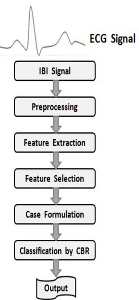
3. Approach and Method
The approach and method comprises of data collection using software prototype and other third party software and tools, preprocessing, feature extraction and selection, feature calculation and Case formulation for CBR implementation that represents in Figure 2.
Figure 2: Steps of the work
3.1 IBI Signal and Preprocessing
Electrocardiography (ECG) signal will be taken from the patient using ECG sensor. A software prototype is needed to collect the data from the sensor to a computer system and calculate the Inter Beat Interval (IBI) signal from the ECG signal. The feature
12
will be extracted from the IBI signal. But IBI signal is frequently contaminated by outliers resulted from the loose conduction of electrodes connected to the body by shaking, itching and sneezing that produces phantom beat or misses some beats of the heart. So, the preprocessing will be to remove outliers from the IBI signal.
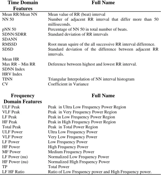
3.2 Feature Extraction
In HRV analysis the features can be time domain features or frequency domain features. The time and frequency domain features are listed in Table 1. Time domain features represent the analyses of the variation between beat to beat. But the frequency domain features give the analysis on frequency spectral of the signal.
Time Domain Features
Full Name
Mean RR/Mean NN Mean value of RR (beat) interval
NN 50 Number of adjacent RR interval that differ more than 50 milliseconds.
pNN 50 Percentage of NN 50 in total number of beats. SDNN/SDRR Standard deviation of RR intervals
SDANN
RMSSD Root mean squire of the all successive RR interval difference. SDSD Standard deviation of the difference between adjacent RR
intervals. Mean HR
Max RR – Min RR Deference between highest and lowest RR interval. SDNN Index
HRV Index
TINN Triangular Interpolation of NN interval histogram
CV Coefficient in Variance
Frequency Domain Features
Full Name
ULF Peak Peak in Ultra Low Frequency Power Region VLF Peak Peak in Very Frequency Power Region LF Peak Peak in Low Frequency Power Region HF Peak Peak in High Frequency Power Region Total Peak Peak in Total Power Region
ULF Power Ultra Low Frequency Power VLF Power Very Low Frequency Power LF Power Low Frequency Power HF Power High Frequency Power MF Power Medium Frequency Power
LF Power (nu) Normalized Low Frequency Power HF Power (nu) Normalized High Frequency Power
TP Total Power
LF HF Ratio Ratio of Low Frequency power and High Frequency power.
13
The IBI signal constructed from ECG signal is time domain signal. But for getting frequency domain feature that signal need to convert into the frequency domain. For doing so, Discrete Fourier Transformation (DFT) is implemented on it. The Fast Fourier Transformation (DFT) is the numerical analysis method to implement FFT to reduce the time complexity. ‘Cooley–Tukey FFT Algorithm’ that is used very commonly as a FFT algorithm among all existing is used here for the time to frequency domain transformation.
But the target is to reduce the number of feature and increase the performance of the CBR system as much as possible. So, a survey was done over 22 articles on HRV analysis to choose features for our experiment. The range of the power spectrum in frequency domain calculation can vary also. The equation for normalization of LF and HF power also differs from article to article. The results of our study are presented in the Tables 2, 3, 4 and 5.
Features Used in Article Number of articles Mean NN [1], [18], [23]-[24] ,[26]-[27], [30]-[33] 10 NN50 [30] 1 pNN50 [1], [4], [16], [18], [21], [23]-[24], [26] 8 SDNN [1], [18], [23], [24], [26]-[27], [30]-[33] 10 SDANN [26], [30] 2 RMSSD [1], [4], [18], [22], [23], [26]-[27], [30], [32]-[33] 10 SDSD [30], [31] 2 HR [18], [23], [32]-[33] 4 Mean NN [1], [18], [23], [24], [26]-[27], [30]-[33] 10
Table 2: List of the Time Domain features that are used in HRV analysis
Features Used in Article Number
of articles ULF Peak 0 VLF Peak 0 LF Peak [20] 1 HF Peak [20] 1 Total Peak 0 ULF Power [30] 1 VLF Power [2], [4], [23], [26], [28], [30], [33] 7 LF Power [1]-[4], [6], [19], [21]-[32] 19 MF Power [25] 1 HF Power [27], [30], [31], [33] 7 Total Power [27], [28], [30] 3 LF/HF Ratio [23], [24], [26]- [31], [33] 13
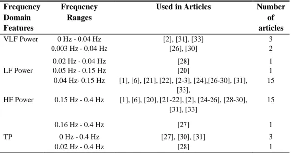
14 Frequency Domain Features Frequency Ranges
Used in Articles Number of articles VLF Power 0 Hz - 0.04 Hz [2], [31], [33] 3 0.003 Hz - 0.04 Hz [26], [30] 2 0.02 Hz - 0.04 Hz [28] 1 LF Power 0.05 Hz - 0.15 Hz [20] 1 0.04 Hz- 0.15 Hz [1], [6], [21], [22], [2-3], [24],[26-30], [31], [33], 15 HF Power 0.15 Hz - 0.4 Hz [1], [6], [20], [21-22], [2], [24-26], [28-30], [31], [33] 15 0.16 Hz - 0.4 Hz [27] 1 TP 0 Hz - 0.4 Hz [27], [30], [31] 3 0.02 Hz - 0.4 Hz [28] 1
Table 4: Lists of the Frequency ranges used in HRV analysis
Equation used for normalizing LF and HF Used in Article
LF (nu) = LF/(LF+HF) [22]
LF (nu) = LF/Total Power, HF (nu) = HF/Total Power
[27]
LF (nu) = LF/(TP-VLF)*100, HF (nu) = HF/(TP-VLF)*100
[30]
Table 5: List of the equations that are used for normalizing LF and HF in the HRV analysis
3.3 Feature Selection
HRV is a popular method to analyze the activities of the Heart and the autonomic nervous system in humans. The state of the ANS is reflected in the HRV. For this reason we chose HRV as one of the key criteria to diagnose stress.
Now, HRV can be analyzed using both time domain and frequency domain attributes. It is very important to choose such features which vary with the changes in the stress level and show relatively reliable behavior. Among many such features here in our case we are choosing some and why we choose them is explained below.
Spectral analysis of HRV can be used for assessing levels of parasympathetic and sympathetic activities in the ANS. For a short term HRV signal we first obtain its PSD (Power Spectrum Density) by means of a Fourier transform. The activities in the frequency range 0.04 to 0.15 are basically termed as LF and are generally due to sympathetic activity with a minor parasympathetic component. The activities in the frequency range 0.15 to 0.5 are basically termed as HF and are generally associated with respiratory sinus arrhythmia and are almost exclusively due to parasympathetic
15
activity. The LF/HF ratio has been used as a measure of sympathovagal balance. If the balance is disturbed by stress then it is reflected in this ratio [43].
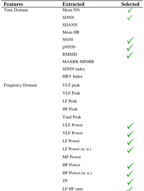
Features Extracted Selected
Time Domain Mean NN
SDNN . SDANN Mean HR NN50 pNN50 . RMSSD . MAXRR-MINRR SDNN index HRV Index Frequency Domain ULF peak
VLF Peak LF Peak HF Peak Total Peak ULF Power VLF Power LF Power LF Power (n. u.) MF Power . HF Power HF Power (n. u.) . TP LF HF ratio .
Table 6: Features extraction and selection
Overall, heart rate variability spectra during baseline conditions are dominated by high frequency activity, a reflection of parasympathetic efferent neuronal innervations and linkage to the ventilatory cycle manifested as respiratory sinus arrhythmia. So typical normal ratio might be something less than 1 and it can go up to 1.5 in young subjects. Stress is accompanied by an increase in the PSD of LF and decrease in PSD of HF. So with stress the ratio’s value rises up. So LF, HF, and the ratio of them are our high priority indices to diagnose stress.
16
Similarly we also use other time domain signals to assist the diagnosis. We try to use such indices which wouldn’t vary hugely between different people in similar conditions. So we consider features which value fluctuations in the HRV. Along with this it is also important that these indices fluctuate in different conditions with some reliable pattern. So we chose SDNN (Standard deviation of all NN intervals), pNN50 (Percentage of differences between adjacent NN intervals that are greater than 50 ms) and RMSSD (Square root of the mean of the squares of differences between adjacent NN intervals) after a close observation of our data. The feature extracted by Discrete Wavelet Transformation are also considered and named as ‘Time-Frequency’ domain feature. For a patient we will consider 5 conditions (among RO2-6) and 17 features each. So we will have 5*17=85 features set from HRV. This will be used to form the case library in our final CBR system. It will also have the stress level that is decided by the expert. The selected features except DWT (Discrete Wavelet Transformation) features are given in Table 6 where mostly used features are selected based on the study.
FFT only gives the available frequencies that are available in the signal. But it does not give the time of the existence of the frequency in the signal. Again the value of the frequency spectral is also the proportional value than the real.
Equation 1: Fourier Transformation
The above equation (1) is the general equation of Fourier transformation where the integration is performed full time interval of the signal. So, Fourier transformation is good when signal is stationary but not that much good when the signal is non-stationary. But IBI signal is very much non-stationary and that is why the Fourier Transform performed on it does not give good result. So, an alternative solution of it can be Short Time Fourier Transformation and Discrete Wavelet Transformation is even better. In Discrete Wavelet Transformation frequency is represented along with the time. So, features extracted by the DWT can be considered as Time-Frequency domain features.
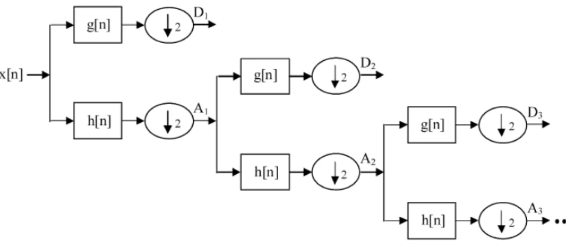
But a previous work [43] shows that there is no significant difference in the value of the LF, HF, and ULF, VLF calculated by FFT and DWT for IBI signal. So, different kinds of features are chosen for DWT that are used in [40]-[42]. ‘Daubechies 4’ or D4 is chosen as a DWT algorithm for the transformation. The algorithm can calculate the coefficient up to level N where the numbers of data points are 2N. But the coefficients are calculated up to level 4 because after that level the values of the coefficients become very small that almost equal to zero. The maximum value, minimum value, mean value and standard deviation of each level are considered as DWT features.
17
Figure 3 shows the decomposition by DWT where signal is passed through a high pass filter and low pass filter. The coefficients are taken from high pass filter and the output of low pass filter is passed again through high and low pass filter for next level of transformation. The list of features calculating from DWT is given in Table 7.
Level Features
D1 Max, Min, Mean, Standard Deviation D2 Max, Min, Mean, Standard Deviation D3 Max, Min, Mean, Standard Deviation D4 Max, Min, Mean, Standard Deviation
Table 7: The list of DWT features [40]-[42].
Figure 3: The Decomposition steps of Daubechies Discrete Wavelet Transformation [40]-[42].
3.4 Data Collection and Prototype Implementation:
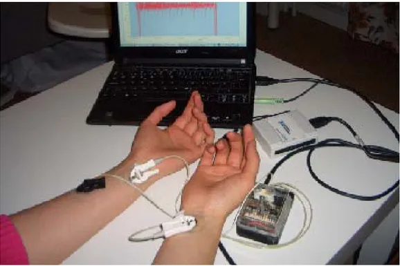
The ECG signals are collected for CBR is by ‘cStresse’ that is a third party software and device. The software also calculates the IBI and HR. This data are then sent to the expert and then classified by him/her. The features are calculated by the software prototype [17] is also capable to take the ECG signal from an ECG sensor and convert it into IBI and HR. Outliers removing is also implemented in the software prototype. So, it has the capability of reading raw ECG signal and calculating IBI and HR from it, calculating Time domain, Frequency domain and Time-Frequency domain features before and after outliers removing. It is also capable to do the same for the data taken by ‘cStress’. More details about the software prototype and CBR are presents in implementation section of the report.
18
3.5 Preprocessing and Getting IBI
Once the Inter Beat Interval (IBI) data is computed from Electrocardiography (ECG) signal, several time domain and frequency domain features are extracted from it. The standard deviation of the IBI (SDNN), root mean square of the difference between adjacent IBI (RMSSD) and percentage of IBI which vary by more than 50 ms from the previous IBI (pNN50) are some of the important time domain features which are mostly used to represent HRV. Similarly, after applying Fast Fourier Transformations (FFT) and performing power spectral analysis, several more parameters like low frequency component (LF), high frequency component (HF) and ratio between LF and HF are also considered to represent HRV effectively [1]. Frequently, IBI data is contaminated by outliers or artifact that is produced by activities like sneezing, shaking the electrodes of ECG sensor or other irregularities. Researches show that some HRV parameter values, which can be very important for HRV analysis, can be changed by a huge percentage for a very small percentage of outliers in the IBI signal. According to the observations made by [1], outliers which accounted less than 0.1 % of total IBI resulted in 45% to 50% anomalies in some of the HRV parameters. As such many researchers have suggested various strategies to identify and handle these outliers that contaminate the IBI data. Many cardiologist and researchers recommend visual inspection of the ECG signal for the outlier’s identification process. But with the increasing length of the signal this process becomes time consuming and expensive. Many commercial products are identifying outliers, but they do not show openly, how they are actually doing it. Many publications also fail to explain the strategies used to filter IBI before the extraction of the features [1]. However, some of the common strategies used by many researchers in the field of HRV analysis identify outlier as those values which are:
--Above 1800 ms or below 300 ms [9] (threshold might vary depending upon the population)
--Some level of percentage change from the mean of some amount of previously accepted IBIs.
--Some well chosen multiple of standard deviation (SD) away from the mean of some amount of previously accepted IBIs [1], [10].
After identifying the outliers, another important task is handling them. There are generally two ways to do it viz. ‘Tossing’ and ‘Interpolation’ [1]. Tossing is the simple process of just removing the data points that are identified as outliers. This is easy to use and a fast process. Some affected data points are lost in this process. However, some researchers consider the continuity of the signal might be important for HRV analysis [9]. Thus to prevent this loss, interpolation is widely popular. Various different kinds of interpolation algorithms are tried upon and tested in this
19
process by many researchers. Here we are particularly interested in observing the impact on HRV parameters by replacing the outliers by equal time spanned, previously accepted data.
First the signal is divided into few portions that are known as windows. In every window the mean is calculated by considering those data points that lie closely together giving high density of points. For doing so, each horizontally split window is again split into few portions vertically. The number of data point of each portion is counted. The mean is calculated by considering only the data points lying in the vertical portion, where the number of data points is the highest. This mean is closer to the expected mean and not affected by high or low values of outliers. The reason is that, the outliers are found in the signal in a tiny number and lie far from the good data points containing very high or low value than the expected or good data points [1],[15]. The technique describes on figure 4 and 5. In figure 4, the signal is split into few windows and calculate mean for every window. The mean of a particular window is considered only for portion of the signal in that window. Then the data of each window deviate less from its local mean than the overall mean.
Figure 4: Mean values calculation by sliding the window.
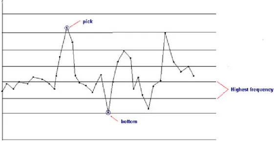
Every window will be again split vertically into several portions as shown in figure 5. Then the frequency for each part is calculated. The average value of the highest frequency region is the 1st best mean. Similarly, 2nd best, 3rd best is calculated and so on. But the 1st best mean is the standard mean for that window. By this way the effect of noises in mean consideration is avoided.
20
Figure 5: Mean value calculation by considering the highest frequency.
Then outliers are removed form that window before going to the next window. The data point that deviates more than the threshold value from the mean of that window is detected as outlier. The consecutive data points that are outliers are counted and replaced by the data points which are good points and available just before these points. If same number of data points is not available before the outliers then the replacing is done by using the data points that lie just after the outliers. The mean calculation, outlier detection and replacing outliers by the data points continue for all the remaining windows in sequence. The given process is shown in Figure 6.
Figure 6: Proposed algorithm to detect and replace outliers.
BEGIN:
1. Split the signal into windows. 2. Select a window and continue.
3. Split the window vertically into ‘n’ equal windows & calculate the means for each window.
4. Determine best mean i.e. the mean of the window containing the highest number of data points.
5. Compare each data point with the best bean.
6. If the data points deviate from best mean more than threshold value than determine them as outliers.
7. Replace all bunches of outliers by bunches of good data points that are available before or after the bunch of outliers.
8. IF next window is available THEN select next window and GOTO step 3, ELSE GOTO step 9.
9. RETURN filtered signal. END.
21
Figure 7 depicts the performance of the algorithm on a IBI signal contaminated by outliers and it illustrate that the algorithm is capable enough to remove the outliers by interpolating with good nearest data points where the other good data points are not hampered.
Figure 7: Removal of outlier by replacing it with previously accepted adjacent data points
The average values of each features for ‘good samples’, ‘bad samples’ and ‘repaired sample’, for an individual S1, are shown in Table 8. This table gives us the idea how values of each features varies for good, bad and the corrected samples. This is calculated for all the individuals before proceeding further.
The Euclidean distances calculated for outlier contaminated IBIs before and after correction, were taken with respect to the feature sets obtained from ‘good samples’. Table 9 represents the distances for feature sets obtained for bad samples by taking only time domain features into consideration. This table allows us to watch the effect of the outliers in the time domain features. The effectiveness of the outlier removing process for the same can also be observed in this table. Similarly Table 10 shows the distances measured by considering only frequency domain features.
This is to view the effectiveness of the outlier removal process in the frequency domain features. Finally, the distances based on both time domain and frequency domain features are presented in Table 11, which gives us an overall picture of the affect of outlier removal in the features.
Features G B R MeanNN 775.76 698.83 786.38 SDNN 33.64 237.89 44.44 pNN50 3.46 23.04 14.80 RMSSD 26.48 162.03 38.28 LF 1.09 1.4 1.09 HF 0.23 0.45 0.23 LF/HF 4.67 3.19 4.67
Table 8: Average values of features extracted from ‘good’ sample G, ‘bad sample’ B and ‘repaired
22
Samples Before correction After correction
S1 257.66 22.29
S2 262.25 25.65
S3 246.65 21.84
Table 9: Distances between ‘good sample’ and ‘bad sample’ based upon the Time Domain features
before and after correction
Samples Before correction After correction S1 1.53 0.003 S2 1.62 0.005 S3 1.42 0.003
Table 10: Distances between ‘good sample’ and ‘bad sample’ based upon the Frequency Domain
features before and after correction
Samples Before correction After correction
S1 257.67 22.29 S2 262.25 25.65 S3 257.67 21.84
Table 11: Distance between ‘good sample’ and ‘bad sample’ based upon all the Features before and
after correction
From Tables 9 and 10, it is observed that the effect of outliers on frequency domain features is relatively very less compared to time domain features. The reason is that outliers are common in samples but rarely available inside the IBI signal [1], [15]. So generally, the percentage of outlier in the sample is very low and this is insufficient to make a huge impact on frequency features. That is why the trend of HRV analysis is mostly based on frequency domain features as implied by Table 2 and 3 in section 3.2. But time domain features are the statistical changes and deviations from beat to beat. That is why the effect of a tiny percentage of outliers is huge. Most of the data are very close and sharp edges are frequent. So common outliers filtering technique would perform very poorly as most of the data should not be changed, except the outliers. Good data should not suffer or get lost. The process discussed in the report is capable to do so as depicted in Figure 7.
Table 10 shows that for frequency domain, the features value become so close to the expectation that the distance is almost zero.
So, from the result we see a good chance for the approach presented in the paper to be used when it comes to remove outliers in IBI signal. But the limitation is that the observation is based on very small number of data and also, all the features are not considered in the analysis. The future work can be performing an experiment in
23
bigger population by considering almost all the features used in HRV analysis. Results from other existing work for outliers removing should also be considered and compared with this approach.
3.6 Case Representation
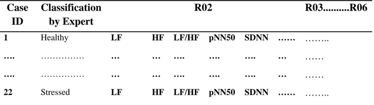
A case consists of six features for each step as clearly shown by Table 12. The steps from RO2 to RO3 are included so that all together a case will have 85 features. It will also contain the classification value from the expert (or in future the determined classification value by the system) along with its case Id.
Table 12: Case representation
3.7 Similarity Function
The general similarity function is shown in Equation 2. ‘Similarity(C,S)’ is global similarity function for new case ‘C’ and stored case ‘S’ and ‘sim(Cf,Sf)’ is local similarity function. Similarity is given in a value between 0 to 1 where 0 means no similarity and 1 means 100% similarity. Similarity is calculated based on calculating simple Euclidian distance, normalizing it and then subtracting it from 1. Similarity is also calculated by using fuzzy similarity. But fuzzy similarity is mainly used here for the evaluation of the CBR as the outcome of it is better over similarity calculated using Euclidian distance [34]. This is done for all the features. Some weights are given to each feature and then the similarity is calculated for a step. Finally weights are given to all the steps as well and then the total similarity value is calculated.
Equation 2: Similarity Equation
Where, and is the local weight for each feature. In the case of Euclidean distance the similarity for each feature i.e. is calculated by
Case ID Classification by Expert R02 R03...R06 1 Healthy LF HF LF/HF pNN50 SDNN …… …….. …. ……… … … …. …. …. … …… …. ……… … … …. …. …. … …… 22 Stressed LF HF LF/HF pNN50 SDNN …… ……..
24
normalizing the absolute difference between the two features for these two cases and dividing it by the difference of the maximum and minimum distance. Finally it is subtracted from 1 to get the similarity. Equation 3 represents this calculation but it is not required for fuzzy similarity.
Equation 3: Normalization to get similarity by using Euclidean distance.
Finally we have similarities for all the steps. Now we again use different weights for each step and calculate the final similarity.
Total Similarity = Similarity for step R02 + Similarity for step R03 + Similarity for step R04 + Similarity for step R05 + Similarity for step R06. where, and is the local weight of a particular step i.e. from RO2 to RO6.
Figure 8: Fuzzy Similarity using triangular membership function [34] [35]
The old and new features values are crisp values that convert in fuzzy by using a triangular member function where the membership grade of 1 at the singleton. Now if m1, m2 and om are the elements of the converted fuzzy set that showed in Figure 8 then the areas of them are calculated and the Equation 4 is used to calculate the similarity.
25
4. Implementation
The approach is to use some sensor hardware to first capture the IBI signals from a patient for 15 min, which consists of 6 sub-parts. The first 3 min is called as the base line and used to adjust the patient’s temperament. Then for the next 2 min (R02) the patient is asked to be relaxed and do positive thinking and remain calm. It is followed by 4 min (R03) of stress session where the patient is told to read some paper and asked to simulate stress condition. After this there is another 2 min (R04) of relaxation session. Then comes the 2 min (R05) math stress session where the patient will be asked math questions. Then finally there is another 2 min (R06) relax session. After this the signal is filtered in order to remove outliers that will seriously affect the information to be retrieved from it. A new method to remove the outliers in the signals has been implemented in this step. Finally, HRV features are extracted based on both time domain and frequency domain analysis. Using these features we formulate a case which is evaluated by the expert and given a stress value. We use HRV features because in biomedical society it is strongly believed that HRV represents the ANS very closely and thus it can be used as an important tool to diagnose the stress levels [2]. When a new case arises, the system compares it with all the cases in the case library and finds the closest case. The stress level of the closest case would very closely reflect the stress level of the new case.
4.1 Software Prototype Implementation
The data are collected through a third party software and device package named ‘cStress’ that is capable to do HRV analysis from the ECG signal by both time and frequency domain features calculation and it gives the feature value of almost all the prominent features in those mentioned domains. But we have implemented our software prototype that describe in [17] and data collection by the software prototype is shown in Figure 9.
Java native interface (JNI) is used as a technique of communication between the Java application and the available code for communicating with the device that written in C language.
26
Figure 9: Data Collection by using software prototype
--It collects ECG data from the patient and calculates IBI and HR where the calculation is done in online that is shown in Figure 10 and 11.
27
Figure 11: Online graph of IBI Signal calculated from ECG Signal
--It can remove outliers from the IBI signal by using the technique mentioned here.
Figure 12: Calculated frequency domain features
--It can calculate the features in time, frequency and time-frequency domain. It converts time domain signal to frequency domain signal by FFT and then calculates the features. A DWT transformation is implemented for calculating the time-frequency domain features that are relatively new and not commonly available in other software prototype where that features will be available with the features that
28
are calculated in simple time and frequency domain. The snap shot of calculated frequency domain features by using the software prototype is shown in Figure 12. --It calculates the features both before and after outliers removing and provides graph and required data that illustrates in Figure 13. Finally it saves the data in database.
Figure 13: Original and Filtered (After removing outliers) IBI
4.2 CBR
Implementation
The CBR is developed by using PHP and MySql. CakePHP is chosen as a Model-View-Controller (MVC) framework that helps to analysis, develop, and maintain the parts of the system easily, rapidly and in well organized way. Figure 14 shows the Entity-Relationship (ER) diagram for our CBR system.
29
Figure 14: ER Diagram of CBR system
The architectural diagram of the system represented in Figure 15 is as like as a typical MVC architectural diagram due to use the CakePHP framework.
The basic idea of the thesis is to construct a CBR system and try to evaluate the accuracy of the system diagnosis compared to the expert diagnosis. To begin with our case has 22 cases in the case library. For each case we have stress value determined by the expert. Now we take one case from the main library as a new case and then match it with every case in the library. Finally the CBR will give a list of similar cases in descending order. Similarity is calculated using simple Fuzzy distance for all the features considered. Finally the stress level of the most closely matched cases is compared with the stress level of the new case. This step allows us to determine the accuracy of the system as well. The diagram in Figure 16 explains the general working of the CBR system involved.
30
Figure 15: MVC System Architecture
31
5. Result and Evaluation
The system was evaluated with 22 case representations. Among these 22 cases, 1 was taken as new case and rest 21 were then taken one by one to match with the current new case. The cases were classified in to 5 stress levels viz. -2, -1, 0, 1 and 2.
The levels of stress -2, -1 are categorized as ‘stressed’ and 0, 1, 2 are categorized as ‘Healthy’. Cases are classified by the expert based on the biological signal Finger Temperature (FT), Hear Rate (HR) and Respiration Rate (RR) individually. Finally all cases are classified after all three biological signals taking in consideration. The classifications are shown in Table 13.
Case Id FT HR RR Combination of FT, HR, and RR
1 Healthy Stressed Stressed Stressed 2 Stressed Stressed Stressed Stressed
3 Healthy Healthy Stressed Healthy 4 Stressed Stressed Stressed Stressed
5 Healthy Healthy Stressed Stressed 6 Stressed Healthy Stressed Stressed
7 Healthy Healthy Stressed Healthy 8 Healthy Stressed Healthy Healthy
9 Stressed Healthy Healthy Healthy 10 Stressed Healthy Healthy Healthy
11 Healthy Healthy Healthy Healthy 12 Stressed Healthy Healthy Healthy
13 Healthy Healthy Stressed Stressed 14 Stressed Healthy Healthy Healthy
15 Healthy Healthy Stressed Healthy 16 Stressed Stressed Healthy Stressed
17 Stressed Healthy Healthy Healthy 18 Healthy Healthy Healthy Healthy
19 Healthy Healthy Healthy Healthy 20 Healthy Healthy Healthy Healthy
21 Stressed Stressed Stressed Stressed 22
Stressed Stressed Healthy Stressed
Table 13 : Classification of the cases based on FT, HR and RR individually and based on all three
biological signal where 'H' represents 'Healthy' and 'S' represents 'Stressed'
If classifications based on individual biological signal are taken in consideration to compare to the overall classifications based on all three biological signals then Figure 17 represents
32
closeness of expert's classification of cases based on individual biological signal to his/her final classification based on all biological signals in percentage.
Figure 17: Expert’s overall classification compared to classification obtain from individual biological
Signal
Now the next concern is to evaluate the system classification of the cases based on HR where weight play is an important role because all the features, steps and domains are not equally important. The weight is mainly given on the features level, step level and domain level. The weights of the each step, time domain features and, frequency domain features is given on the basis of our study and previous related work that are listed on Table 14, 15 and 16 respectively.
Step Number
Step Name Duration Weight
R02 Relax 2 minutes 10
R03 Stress 4 minutes 6
R04 Relax 2 minutes 9
R05 Math Stress 2 minutes 6
R06 Relax 2 minutes 6
Table 14: Step of the Weight List
Feature Name Weight Beats 0 Mean NN 10 NN50 1 pNN50 9 SDNN 10 RMSSD 10
33
Feature Name Weight ULF Peak 0 VLF Peak 0 LF Peak 0 HF Peak 0 Total Peak 0 ULF Power 1 VLF Power 8 LF Power 10 LF Power (nu) 7 HF Power 10 F Power (nu) 7 LF HF Ratio 9 Total Power 3
Table 16: Frequency Domain Weight List
For time-frequency domain the DWT (Daubechies 4) is done up to 4 levels because in the rest of the level the coefficient is as too small as close to zero [41]. The first level (D1) is related to standard deviation. Every level the features set are comprise of four values as Max (Maximum), Min (Minimum), Mean and Standard deviation of the coefficient of that level. So weights are put according to the level as well as to the feature value. The features are chosen by the study on related article that works on DWT feature extraction from ECG [41]. Weight is same for each feature of each level that is shown in Table 17 but the weight of the level is determined by the evaluation of the CBR.
Feature name weight
Max 1 Min 1 Stddev 1
Mean 1
Table 17: Frequency Domain Weight List
If every time one level of DWT transformation is only taken in consideration then the outcome for first level (D1) is shown in Table 18 and the summary of all 4 level and their combinations are shown Table 19.
34
Case id Expert System If expert = system then 1 else 0 1 Stressed Healthy 0 2 Stressed Stressed 1 3 Healthy Healthy 1 4 Stressed Healthy 0 5 Healthy Healthy 1 6 Healthy Healthy 1 7 Healthy Healthy 1 8 Stressed Stressed 1 9 Healthy Healthy 1 10 Healthy Healthy 1 11 Healthy Healthy 1 12 Healthy Healthy 1 13 Healthy Healthy 1 14 Healthy Healthy 1 15 Healthy Healthy 1 16 Stressed Healthy 0 17 Healthy Healthy 1 18 Healthy Stressed 0 19 Healthy Healthy 1 20 Healthy Healthy 1 21 Stressed Healthy 0 22 Stressed Healthy 0 Correctly Classified 73%
Table 18: CBR evaluation for DWT where weight of level 1 = 100%.
Level of DWT Number of features (each step) Total Number of features in a case Correctly classified D1 4 20 73% D2 4 20 64% D3 4 20 73% D4 4 20 50% D1, D2, D3, D4 16 80 63% D1, D2, D3 12 60 68% D1, D2 8 40 68% D1, D3 8 40 73%
Table 19: CBR evaluation of DWT for each level and combination of various levels.
From the observation on Table 19 only level 1 (D1) features are taken in consideration for evaluating the system and the weight of the first level is 100% where weight for all other levels are zero because individually level D1 and D3 as well as their combination gives same output as for D1 and relatively better output than others but D1 is preferred to reduce the number of features and it has higher precedence than D4.
Then weights mentioned above are applied to the system to evaluate. The Time, Frequency and Time-frequency domain features are considered individually and with
35
their combination to evaluate the system that is listed in Table 20. When the features of a single domain are taking in consideration then the weight of that domain is 100% and all other are zero. In the case of evaluation by considering the combination of domains, weights are assigned in such way that the total importance will be 100%.
Domain Importance of the Domain Correctly Classified Correctly classified on Stress group Correctly classified on of Healthy group Time Time: 100% Frequency: 0% Time-frequency: 0% 64% 25% 86% Frequency Time: 0% Frequency: 100% Time-frequency: 0% 73% 38% 93% Time-Frequency Time: 0% Frequency: 0% Time-frequency: 100% 73% 38% 93% Frequency, Time-Frequency Time: 0% Frequency: 50% Time-frequency: 50% 68% 25% 93% Frequency, Time-Frequency Time: 0% Frequency: 30% Time-frequency: 70% 68% 25% 93% Frequency, Time-Frequency Time: 0% Frequency: 70% Time-frequency: 30% 68% 38% 86% Time, Frequency Time: 40% Frequency: 60% Time-frequency: 0% 86% 57% 100% Time, Frequency Time: 30% Frequency: 70% Time-frequency: 0% 77% 38% 100% Time, Frequency, Time-Frequency Time: 20% Frequency: 40% Time-frequency: 40% 68% 38% 93% Time, Frequency, Time-Frequency Time: 30% Frequency: 50% Time-frequency: 20% 68% 25% 93%
Table 20: Various domains and their combinations are represented with correctly classified cases, miss
diagnosis of stressed and miss diagnosis of healthy
The percentage of correctly classified cases is highest (86%) for the combination of Time and Frequency domain where the weights are 40 and 60 percent respectively and Correctly classified on Stress group (Sensitivity) and correctly classified on of Healthy group (Specificity) are also highest (57% and 100% respectively) for that. But it is so much important to increase the sensitivity then increasing the total accuracy and specificity because it is quite dangerous to diagnose a stressed person as healthy and send him/her to the home without any medication than to diagnose a
36
healthy person as stressed. The reason of lower sensitivity compared to specificity can be the less number of stressed cases compared to the healthy cases where the classification was done by the expert. Only 7 cases are classified as stressed where 15 cases are classified as healthy according to the expert. So, the number of stressed cases is less than half compared to the number of cases classified as healthy. So, the probability of getting higher sensitivity is very less than the probability of getting higher specificity from system evaluation.
In this situation, the probability of a case classified as stressed by the system has tried to increase by increasing the number of stressed case compared to the healthy case in the case library. But when the real life data taken from the patients that are classified by expert is not available, the stressed case can be increased by artificial cases generated from available cases from case library. But HR signal is too complex to ensure that newly generated artificial case should be considered as a stressed case or not and again an expert is needed to do so. So, the alternative is to remove the cases that are classified as healthy by the expert from the case library and generate a new case library where the number of cases classified as stressed higher than that as healthy. For doing so, the cases classified as healthy was removed randomly from the case library to generate new case libraries by 3 individual persons. First the 7~8 cases are removed from the main case library to make a new case library. Then 3~4 cases are again removed from the newly generated case library to make another case library. Both the case libraries make a new set of case library. 4 new class library sets with total 8 new case libraries are generated; those are described in Table 21.
Case library Number of randomly deleted cases Total Number of Cases Number of Healthy Case Number of Stressed Case Probability to be classified as stressed by the system
Main case library 0 22 15 7 0.32
Case library 1 8 14 7 7 0.5 Case library 2 11 11 4 7 0.64 Case library 3 8 14 7 7 0.5 Case library 4 11 11 4 7 0.64 Case library 5 8 14 7 7 0.5 Case library 6 11 11 4 7 0.64 Case library 7 8 14 7 7 0.5 Case library 8 11 11 4 7 0.64
Table 21: The description of case libraries that are generated from main library by reducing the cases
classified as healthy to increase the probability of a case to be classified as stressed.
Case library set 1 comprises case library 1 and 2, Case library 2 comprises case library 3 and 4, and so on.
37
Again to increase the tendency of the system to classify a case as stressed, other n closest cases can be taken in consideration. In our evaluation, 1st, 2nd and 3rd closest cases are taken in consideration. When the evaluation is done only considering the case that is with highest similarity then the value of k is 1. The value of k =2 when the next case with highest similarity is also taken in consideration and so on. When k =1 then there is no other choice but when k = n then the system will take classification of the case that is classified as stressed by the expert for classification from n closest cases if it is available, otherwise the case with highest similarity will be taken for classification.
The evaluations for the case libraries for k = 1, 2 and 3 are shown in the table 22.
Probability of a case to be classified as Correctly classified Cases (%) Sensitivity specificity Case library Stressed Healthy k = 1 k = 2 k = 3 k = 1 k = 2 k = 3 k = 1 k = 2 k = 3 Main 0.32 0.68 86 77 73 57 57 57 100 87 80 1 0.5 0.5 71 64 71 71 71 100 71 57 43 2 0.64 0.36 91 91 73 86 100 100 100 75 25 3 0.5 0.5 71 50 43 57 57 71 86 43 14 4 0.64 0.36 64 64 64 71 100 100 50 0 0 5 0.5 0.5 71 57 43 57 57 71 86 57 14 6 0.64 0.36 55 64 64 57 86 100 50 25 0 7 0.47 0.53 80 73 67 57 71 71 100 75 63 8 0.64 0.36 73 64 55 57 71 86 100 50 0
Table 22: Percentage of correctly classified cases, Sensitivity and Specificity for all the case libraries
Table 23 describes the accuracy of the system classification, sensitivity and specificity according to the size of the class library.
Number of Case in Case Library Number of Case library Mean Accuracy (%) Mean Sensitivity (%) Mean Specificity (%) 22 1 86 57 100 14~15 4 73.25 ± 4.5 60.5 ± 7 85.75 ± 11.84 11 4 70.75 ± 15.37 67.5 ± 13.84 75 ± 28.87
Table 23: The accuracy of the system classification, sensitivity and specificity according to the size of
the class library.
The sensitivity compared to the probability of a case to be classified as stressed for all case library set for k = 1 is shown in Figure 18.
38
Figure 18: Probability of a case to be classified as stressed Vs Sensitivity for class libraries for k = 1.
The sensitivity compared to the probability of a case to be classified as stressed for all case library set for k = 2 is shown in Figure 19.
Figure 19: Probability of a case to be classified as stressed Vs Sensitivity for class libraries for k = 2.
The sensitivity compared to the probability of a case to be classified as stressed for all case library set for k = 3 is shown in Figure 20.
39
The sensitivity compared to the k value for all case libraries is shown in Figure 21.
Figure 21: Sensitivity Vs k value for all case libraries
The accuracy of the system compared to the k value for all case libraries is shown in Figure 22.
Figure 22: Accuracy of the system Vs k value.
The accuracy of the system compared to number of cases in case library is shown in Figure 23.
![Figure 1: CBR cycle [47].](https://thumb-eu.123doks.com/thumbv2/5dokorg/4761546.126783/20.892.207.693.125.617/figure-cbr-cycle.webp)
![Figure 8: Fuzzy Similarity using triangular membership function [34] [35]](https://thumb-eu.123doks.com/thumbv2/5dokorg/4761546.126783/38.892.160.719.445.781/figure-fuzzy-similarity-using-triangular-membership-function.webp)