Sensor fault detection with Bayesian networks
Esin Iplik
Ioanna Aslanidou
Konstantinos Kyprianidis
Automation in Energy and Environmental Engineering, Mälardalen University, Sweden
esin.iplik@mdh.se
Abstract
Several sensors are installed in the majority of chemical reactors and storage tanks to monitor temperature profiles for safety and decision-making processes such as heat de-mand or flow rate calculations. These sensors fail occa-sionally and generate erroneous measurement data that need to be detected and excluded from the calculations. However, due to the high number of process variables dis-played in the chemical plants, this task is not trivial. In this work, a Bayesian network approach to detect faulty temperature sensors is proposed. By comparing the sen-sor measurements with each other, the faulty sensen-sor is de-tected. A modular approach is preferred, and networks are created for 10 K temperature intervals to increase flex-ibility and sensitivity. Created networks can be adjusted for the operating temperature ranges; hence, they can be used for any catalyst and entire life cycle. The devel-oped method is demonstrated on an industrial scale hy-drocracker unit with 92 sensor couples installed in a se-ries of reactors. From the investigated sensors, 16 of them showed a greater difference than the 2 K threshold chosen for the fault. In addition to that, 13 sensors showed an in-creasing temperature difference that may lead to a fault. Two scenarios were created to calculate the energy loss due to a faulty measurement, and a 5.5 K offset error was found to cause a 5.79 TJ energy loss every year for a small scale hydrocracker.
Keywords: Bayesian network, sensor fault, fault detection, diagnostics
Nomenclature
P(a) Probability of an event a
P(a | b) Probability of an event a given event b BN Bayesian Network
CPT Conditional Probability Table DAG Directed Acyclic Graph
1
Introduction
Temperature is one of the most often measured process parameters for several industries. Reaction kinetics are highly dependent on the temperature of the process, mak-ing temperature measurements important for the
chemi-cal industry. These measurements are necessary to have knowledge of the reaction progress for both safety and control. Safety systems rely on the sensors, and wrong measurements can cause a false alarm or dangerous sit-uations. According to the French Ministry of Ecology, Sustainable Development and Energy, sensor failures are responsible for 52% of the accidents in four most au-tomated sectors (refining, metallurgy, food processing, and chemical processing) between 1993 and 2011 (Min-istry of ecology, sustainable development and energy, 2012). Similarly, an optimal operation decision can only be guaranteed by measuring the relevant variables cor-rectly. Faulty measurements do not necessarily cause ac-cidents but waste energy and resources; therefore, sensor failure detection mechanisms are highly important for in-dustrial plants.
Model-based and data-based methodologies are em-ployed to detect sensor faults. While the first one com-pares the expected values calculated by using physical models with the measurements, the latter uses previous measurements to diagnose a failure. In literature, exam-ples for both methods can be found for different applica-tions. A mathematical model consisting of mass and en-ergy balances was used for a central chilling plant’s flow and temperature sensor fault detection (Wang and Wang, 2002). A nonlinear state observer with a mathematical model was tested to detect temperature sensor faults of a heat exchanger (Escobar et al., 2011). The model itself sets the limitation to the model-based approach because its accuracy defines the detection capability. It is sug-gested for the detection of total failures but not for small errors (Du et al., 2009). A data-based approach, an artifi-cial neural network, was used to detect air flowrate sensor faults of a building (Wang and Chen, 2002). Later, a prin-cipal component analysis based fault detection system was developed for temperature sensors of a centrifuge chiller (Wang and Cui, 2005).
Bayesian networks (BN) have gained attention for fault detection as they can show causality. They are found sim-ilar to white-box models due to their qualitative graph as-pect (Hommersom and Lucas, 2010). Although BNs need more information in terms of prior probabilities, they are used for industrial applications. For maintenance plan-ning (Jones et al., 2010), root cause diagnosis of varia-tions (Dey and Stori, 2005), prognosis (Hu et al., 2011) and risk analysis (Duval et al., 2012), these networks were found useful. Their use for fault detection was
success-fully shown on a chiller (Wang et al., 2017), a heat pump (Cai et al., 2014) and a fuel cell (Riascos et al., 2007). A sensor fault detection work was published for a medical body sensor network (Zhang et al., 2016).
The present paper shows a modular BN approach for fault detection of an industrial hydrocracker’s temperature sensors. A modular approach is chosen for this case to cope with the increasing temperature of the system. The operational temperature range is divided into intervals, and a single network is trained for each interval. Further information on the developed strategy is given in the meth-ods section. The results are presented and discussed in the section that follows, and a faulty sensor scenario is created to demonstrate the additional energy consumption due to the fault. Finally, in conclusion section outcomes of this work are summarized next to possible points for future in-vestigations.
2
Methods
Bayesian networks are graphically represented probabilis-tic models, in which every node is assigned to a variable and has its conditional probability table (CPT) depending on its parents (Pearl, 1988). The graphical part of a BN is a directed acyclic graph (DAG). DAG is the qualitative element of a BN, which shows the causality relations be-tween the variables. CPT is the quantitative element that carries the joint probability distribution knowledge, and the posterior probability is calculated according to Bayes’s theorem (Eq. 1).
P(A|B) = P(B|A)P(A)
P(B) (1)
In this work, Bayesian networks are trained for a fault detection system of temperature sensors in a hydrocracker unit. The sensors are distributed in concentric circles as given in Figure 1 in order to observe the temperature pro-file of the catalyst bed. There are four catalyst beds in the reactors, which have identical sensor positioning and all the sensors are thermocouples.
There is a pair of sensors at every point to acquire a reliable measurement, and the average value is used for process calculations. The continuous hydrocracking pro-cess suffers from catalyst degradation; due to this phe-nomenon, the temperature of the system has to increase over time to achieve the same level of cracking. The oper-ation continues ideally without interruption until the end of the catalyst life. Measurements of five representative sensors over two years are given in Figure 2. Each sensor has an average 35 K increase in the measured tempera-ture, and different catalyst beds have different operating temperatures. The measurements from all the sensors are in a 50 K range. Reference temperature (Tre f) is taken as
the start of the run temperature.
A neighboring sensor pair with similar temperature measurements is selected for each location, and their aver-age is used as a reference point to detect a faulty sensor of
Figure 1. Approximate sensor locations on the horizontal cross-section.
Figure 2. Daily data from five sensors for two years.
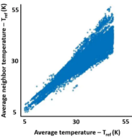
a pair. The average temperature of each sensor is plotted against the average neighbor temperature in Figure 3 to inspect the distribution of the data points in the operation domain.
As Figure 3 clearly demonstrates, there is a trend be-tween the average values that shows well-chosen neigh-bors for each sensor; however, this trend is not entirely linear because of the flow regime, possible hot spots, and channels. If a single network were used to represent this space, the CPT would cover the entire area, most of which have zero probability. The operating temperature range of 50 K that is observed for an entire catalyst cycle is divided into 10 K fragments that are 5 K 15 K, 15 K -25 K, -25 K - 35 K, 35 K - 45 K, 45 K - 55 K based on the average temperature of the pair to reduce the size of the CPT. These values are calculated with the subtraction of the Tre f from the real values. A discrete network is
trained for each range separately by using the data within the range collected from every sensor. Figure 4 shows the range of five networks in different colors and the shaded
Figure 3. Average temperature range with respect to average neighbor temperature.
zero probability area, which proves the reduction of the CPT size.
Figure 4. CPT reduction by modular network approach.
Five networks have identical DAG, which is given in Figure 5. The nodes a and b represent each sensor of a pair, and the neighbor node is the average value of the sen-sors selected for each pair differently. Structural learning of these three nodes is performed by using the necessary path condition algorithm (Steck and Tresp, 1999). Con-sidering the sensitivity of the sensor type, a discretization interval of 1 K is chosen for a and b nodes, and 2 K for the neighbor node. Unlike the interval nodes of the sensors, the fault node and its CPT considering three states (No fault, Fault A, and Fault B) are added with expert knowl-edge, an exemplar CPT is given in the Table 1. For every neighbor, A and B interval, probability of fault states are defined. The fault node’s CPT is a 3D array due to three parent nodes it has, and a high temperature difference of A and B indicates a fault. For example, the temperatures of Neighbor = T, A = T + 0.5, and B = T + 3.5 would result in a 95% probability of ’Fault B’ because the differ-ence is higher than the threshold, and the measurement of sensor A is closer to the neighbor measurement. Hugin, a
Figure 5. DAG of the Bayesian network used for sensor fault detection.
commercial software, is used to build BNs of this work. Different hydrocracking catalysts operate in different temperature ranges. The suggested modular approach brings flexibility to sensor fault detection. A different range can easily be covered by building a new module with the same DAG and a similar CPT; therefore, the networks are easily adjustable and reusable for different catalysts and units. Although a single network for the entire op-eration domain might be useful for higher errors due to its CPT range, it cannot be reused in a different tempera-ture range. Furthermore, a greater CPT range also causes problems. It is hard to fill with expert knowledge if it has the same discretization intervals, or it is not as sensitive if it has the same size as the smaller range CPT. If a sin-gle network were designed for the same system with equal intervals, the fault node’s CPT size would be 187500. In the current design, each fault node has a CPT with 2700 values, and due to the similar trend, they are identical.
A single measurement per day is taken from 92 sensors for two years (684 from each sensor), and they are clas-sified into five intervals of 10 K as described above. The outliers that are values outside the operational range due to some process interruptions are visually excluded from data sets. The five networks are built by using 767, 2494, 10909, 17437, and 17889 points according to increasing average temperature intervals. These networks are tested by using five test data sets of 709, 2436, 10791, 17642, and 17658 values, respectively, 684 measurements from each sensor, excluding the outliers. The test data points are chosen 12 hours after each training data; therefore, the testing is as independent as possible. Both the training and the test data covers the entire catalyst life span.
3
Results and Discussion
The five networks for different temperature intervals are built and tested with real data. According to interval
cal-Table 1. Construction rules of fault node CPT. Neighbor (T-1) – (T+1) A (T) – (T+1) · · · B (T) – (T+1) (T+1) – (T+2) (T+2) – (T+3) (T+3) – (T+4) (T+4) – (T+5) (T+5) – (T+6) · · · No Fault 1 1 0.7 0 0 0 · · · Fault A 0 0 0.05 0.05 0.05 0.05 · · · Fault B 0 0 0.25 0.95 0.95 0.95 · · ·
culus, the built CPT detects an error if there is a difference of at least 2 K. A deviation over 2 K between the pair is detected at 16 of 92 sensors. Each detected fault is inves-tigated separately and found that the difference between the sensor measurements does not change over time. In Figure 6, error with respect to time is given for a pair of sensors.
Figure 6. Temperature difference of a sensor pair, indicating a possible calibration error.
The constant temperature difference over time shows a possible calibration error starting from the installation. The smallest difference detected as calibration error is 2.1 K, and the greatest one is 5.5 K. This type of error may seem harmless since it does not increase over time; how-ever, it can interfere easily with the calculation and appli-cation of optimal operating conditions. Optimality cannot be guaranteed with measurement errors existing in a sys-tem. If a calibration error is detected, it can be eliminated easily.
A calibration error is not the only error type found; an increasing deviation is also observed in faulty sensors. In Figure 7, an example of increasing deviation is given.
Figure 7. Increasing temperature difference of a sensor pair, indicating an error.
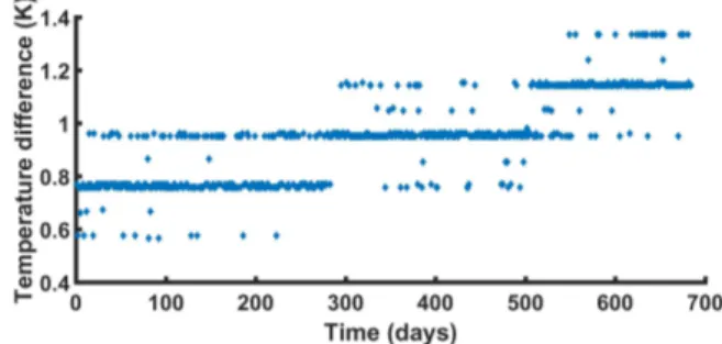
Besides the faulty sensors, 13 sensors are detected with
decreasing reliability, falling into 30% fault probability re-gions of the CPTs. These sensors have no calibration er-ror and have an increasing temperature difference trend. Figure 8 shows the temperature difference increasing over time, which does not pass the error threshold of 2 K. If the same equipment is to be used for the next run of two years, these sensors should be carefully monitored.
Figure 8. Increasing temperature difference of a healthy sensor pair with decreasing reliability.
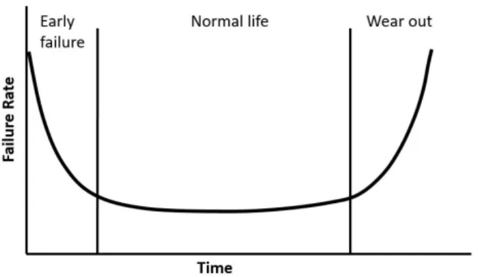
Considering the lifetime of sensors are generally longer than two years, this information can be useful when there is an opportunity for maintenance. When there is a need for a catalyst change, the continuous operation stops for a certain amount of time, and all the reactor content is discharged. The internal equipment maintenance is often scheduled for this period. With the knowledge of calibra-tion error and increasing deviacalibra-tion, relevant sensors can be fixed. The collected data belongs to a new set of sen-sors; therefore, it is expected to have a low rate of faults since sensor faults have a bathtub curve distribution over time (Mishra et al., 2002). A bathtub curve is given in Figure 9, which suggests increasing the importance of a fault detection mechanism with the aging equipment. A fault detection system can simplify maintenance planning because it allows an analysis of the given curve. Consider-ing the age of the sensors, the expected lifetime of the next catalyst, and the number of faulty or less reliable sensors, a decision on whether to keep or change the equipment can be taken. A decision to reuse the same sensor system for the next two years’ run can save the equipment cost; however, an erroneous measurement can increase operat-ing costs.
Tolerance value of a thermocouple is around ±1 K and this value is important to test the robustness of the net-works. Random noise is generated within this range and added to each test measurement. From 49236
measure-Figure 9. Bathtub curve of sensor failure rate with respect to time.
ments, 3.1% are detected false positive and 3.8% are de-tected false negative with the added noise.
Energy loss due to faulty sensors
Two scenarios are developed to calculate the energy loss due to measurement errors, the first one for a faulty sensor, and the second one for a 30% fault probability sensor with an increasing temperature difference trend.
Scenario 1
A small scale hydrocracker unit with 85000 kg/h feed capacity is fed with heavy oil of approximately 30 degrees API (at 60oF) and 2.95 KJ/kg.K specific heat (United States Department of Commerce, Bureau of Standards, 1929). The start of the run temperature of the unit is 650 K, which is an average value for this operation (Ancheyta et al., 2005). A calibration error of 5.5 K decreases the average temperature of the pair by 2.75 K. If this sensor is a feed temperature measurement sensor, which is of-ten a manipulated variable of the control system (Cutler and Hawkins, 1987), this error costs an additional 5.79 TJ energy consumption in a year for a constant temperature operation. As explained earlier, in reality, the system tem-perature increases as the severity of catalyst degradation increases; therefore, the specific heat increases over time, and the energy loss is higher than the calculated value.
Scenario 2
The same hydrocracker unit sensor has an increasing temperature deviation, which does not exceed the fault threshold yet, but it is in the 30% fault region. Its tem-perature difference increases by 0.2 K every four months, starting from 1 K to 2 K at the end of two years. It de-creases the average temperature by 0.5 K in the first four months, causes an additional 0.361 TJ consumption. In the next five periods of four months, this value increases to 0.433 TJ, 0.505 TJ, 0.578 TJ, 0.65 TJ, and 0.722 TJ. In total, it might cause an additional consumption of 3.25 TJ in two years.
These two scenarios show why sensor faults need to be detected as early as possible. They both consider the fault in a negative direction. A fault that increases the average
temperature can cause other problems, for example, inef-ficient cracking. In the case of the lower temperature of the reactor feed, the cracking reactions cannot be carried out at the desired rate, and the product specifications can-not be reached. Therefore, the outputs of the process need further processing, and so additional energy need arises that increases the production cost.
An important point to consider is the limitations of the designed network system. As mentioned earlier, this type of limited range network cannot identify the significant er-rors, which throws the average out of the operational do-main. It can be overcome by using high range buffer inter-vals as the first and the last elements of the CPT. This ad-dition allows the BN to function in a higher range without expanding it significantly. As the targeted errors are high in value, the buffer zones do not need high sensitivity, so it is easy to detect them if the network can be evaluated with the given measurements. Another issue to be considered is the reliability of the neighbor sensors’ measurements. If there is a faulty neighbor, it will still be possible to detect a fault, but it will not be possible to detect which sensor is faulty. A weighted average of multiple measurements can be used as the reference point to reduce this problem.
4
Conclusion and Future Work
Five Bayesian networks, each addressing a different tem-perature interval, are designed to detect a hydrocracker reactor’s sensor faults. A set of data collected from 92 sensor pairs and their closest neighbors is used for train-ing the networks, and a fault node is added with expert knowledge. Developed networks are tested with data, and 16 sensors are detected with an error greater than 2 K. Detected faulty sensors are investigated, and two types of faults are found in the system, offset errors and increas-ing errors. In addition to the faulty sensors, 13 sensors are detected with decreasing reliability, although their differ-ences are lower than the fault threshold of 2 K. Two energy loss scenarios are used to demonstrate the importance of detecting both the erroneous measurements and the small deviations. BN is a fast tool that can be built both from data and by expert knowledge that gives it flexibility, and in this work, it is demonstrated that BNs can be used to de-tect sensor failure. With the increasing interest in it, BNs might help different industries operate safely without en-ergy losses. Future work on the same system with special attention on the sensors that have an increasing tempera-ture deviation can justify the reliability of this prognosis. The limitations discussed, significant errors’ detection and neighbor faults, should be solved to build a reliable sensor fault diagnostics system. In addition to that, a dynamic Bayesian network, which considers the previous error, can be used to distinguish the increasing errors from the offset errors.
Funding:This research was a part of FUDIPO project and funded by European Union’s Horizon 2020 Research and Innovation Program under grant number 723523.
References
Jorge Ancheyta, Sergio Sánchez, and Miguel A Rodríguez. Ki-netic modeling of hydrocracking of heavy oil fractions: A review. Catalysis Today, 109(1-4):76–92, 2005.
Baoping Cai, Yonghong Liu, Qian Fan, Yunwei Zhang, Zengkai Liu, Shilin Yu, and Renjie Ji. Multi-source information fu-sion based fault diagnosis of ground-source heat pump using Bayesian network. Applied energy, 114:1–9, 2014.
CR Cutler and RB Hawkins. Constrained multivariable control of a hydrocracker reactor. In 1987 American Control Confer-ence, pages 1014–1020. IEEE, 1987.
Story Dey and JA Stori. A Bayesian network approach to root cause diagnosis of process variations. International Journal of Machine Tools and Manufacture, 45(1):75–91, 2005.
Zhimin Du, Xinqiao Jin, and Yunyu Yang. Fault diagnosis for temperature, flow rate and pressure sensors in vav systems using wavelet neural network. Applied energy, 86(9):1624– 1631, 2009.
Carole Duval, Geoffrey Fallet-Fidry, Benoît Iung, Philippe We-ber, and Eric Levrat. A Bayesian network-based integrated risk analysis approach for industrial systems: application to heat sink system and prospects development. Proceedings of the Institution of Mechanical Engineers, Part O: Journal of Risk and Reliability, 226(5):488–507, 2012.
RF Escobar, CM Astorga-Zaragoza, AC Téllez-Anguiano, D Juárez-Romero, JA Hernández, and GV Guerrero-Ramírez. Sensor fault detection and isolation via high-gain observers: Application to a double-pipe heat exchanger. ISA transac-tions, 50(3):480–486, 2011.
Arjen Hommersom and Peter JF Lucas. Using Bayesian net-works in an industrial setting: Making printing systems adap-tive. In ECAI, pages 401–406, 2010.
Jinqiu Hu, Laibin Zhang, Lin Ma, and Wei Liang. An inte-grated safety prognosis model for complex system based on dynamic Bayesian network and ant colony algorithm. Expert Systems with Applications, 38(3):1431–1446, 2011. B Jones, Ian Jenkinson, Zaili Yang, and Jin Wang. The use of
Bayesian network modelling for maintenance planning in a manufacturing industry. Reliability Engineering & System Safety, 95(3):267–277, 2010.
Ministry of ecology, sustainable development and energy. Ac-cident analysis of industrial automation. Technical report, 2012.
Satchidananda Mishra, Michael Pecht, and Douglas L Good-man. In-situ sensors for product reliability monitoring. In Design, Test, Integration, and Packaging of MEMS/MOEMS, volume 4755, pages 10–19. International Society for Optics and Photonics, 2002.
Judea Pearl. Probabilistic reasoning in intelligent systems. San Mateo, CA: Kaufmann, 23:33–34, 1988.
Luis Alberto M Riascos, Marcelo G Simoes, and Paulo E Miyagi. A Bayesian network fault diagnostic system for pro-ton exchange membrane fuel cells. Journal of power sources, 165(1):267–278, 2007.
Harald Steck and Volker Tresp. Bayesian belief networks for data mining. In Proceedings of the 2. Workshop on Data Mining und Data Warehousing als Grundlage moderner entscheidungsunterstützender Systeme, pages 145–154. Cite-seer, 1999.
United States Department of Commerce, Bureau of Standards. Thermal properties of petroleum products. Technical report, 1929.
Shengwei Wang and Youming Chen. Fault-tolerant control for outdoor ventilation air flow rate in buildings based on neural network. Building and Environment, 37(7):691–704, 2002. Shengwei Wang and Jingtan Cui. Sensor-fault detection,
di-agnosis and estimation for centrifugal chiller systems using principal-component analysis method. Applied Energy, 82 (3):197–213, 2005.
Shengwei Wang and Jin-Bo Wang. Robust sensor fault diagnosis and validation in hvac systems. Transactions of the Institute of Measurement and Control, 24(3):231–262, 2002.
Zhanwei Wang, Zhiwei Wang, Suowei He, Xiaowei Gu, and Zeng Feng Yan. Fault detection and diagnosis of chillers us-ing Bayesian network merged distance rejection and multi-source non-sensor information. Applied energy, 188:200– 214, 2017.
Haibin Zhang, Jiajia Liu, and Nei Kato. Threshold tuning-based wearable snsor fault detection for reliable medical monitor-ing using Bayesian network model. IEEE Systems Journal, 12(2):1886–1896, 2016.