Re-engineering Sequential Software to Introduce Parallelization

(1)

V¨

aster˚

as, Sweden

Thesis for the Degree of Master of Science in Software Engineering

30.0 credits

RE-ENGINEERING SEQUENTIAL

SOFTWARE TO INTRODUCE

PARALLELIZATION

Andreas Granholm

agm11002@student.mdh.se

Examiner: Antonio Cicchetti

M¨

alardalen University, V¨

aster˚

as, Sweden

Supervisors: Federico Ciccozzi and Masoud Daneshtalab

M¨

alardalen University, V¨

aster˚

as, Sweden

Company supervisor: Johnny Holmberg

ABB Robotics, V¨

aster˚

as

(2)

Abstract

In the quest for additional computational power to provide higher software performance, indus-try have shifted to multi-core processing units. At the same time, many existing applications still contain sequential software; in these cases, multi-core processors would not deeply improve per-formances and in general would be under-utilized since software running on top of them are not conceived to exploit parallelization. In this thesis we aim at providing a way to increase the perfor-mance of existing sequential software through parallelization and at the same time minimizing the cost of the parallelization effort. The contribution of this thesis is a generic parallelization method for introducing parallelization into sequential software using multi-core CPUs and GPUs. As a proof-of-concept we ran an experiment in industrial settings by applying the proposed paralleliza-tion method to an existing industrial system running sequential code. Addiparalleliza-tionally, we compare the method we propose to existing methods for parallelization.

(3)

1 Introduction

With the increasing demand of computational power created by modern systems, multi-core pro-cessing units have become increasingly adopted in industry [1]. The reason is that increasing the frequency of the processor to achieve better performance is simply not viable due to physical lim-itations of the single-core chip [2]. Practically, the speed of a Central Processing Unit (CPU) is limited by both heat generation and gate delay of transistors. Instead, in order to increase the performance of digital systems, multi-core processing units are used to run computations in paral-lel, thus increasing the performance of software through parallelization. Today, besides multi-core CPUs, developers have an additional parallel computing platform for general-purpose program-ming at their disposal, namely Graphical Processing Unit (GPU). Initially designed for graphical computations, GPUs offer many more computational units than a multi-core CPU, but with the drawback of generally being slower in terms of clock frequency.

Despite the accessibility to these parallel hardware platforms, many software applications still run code sequentially. In order to utilize the full potential of parallel hardware, existing software needs to be re-engineered to exploit parallelization. As a response to this shift, methods for de-veloping software for parallel as well as distributed systems have emerged [3]. However, parallel software is generally more complex than sequential software [4]. Because of this, developers need more guidance in finding concurrent tasks in existing software [5]. Although there are techniques for automated parallelization, they are not able to produce as good results as an engineer would manually achieve [6]. While there are many tools and programming guidelines available for par-allelization of software, the increased complexity of ”thinking parallel” still poses a problem for software engineers [7].

The goal of parallelizing software is usually to increase the performance, but by doing this other quality attributes are usually affected, often negatively. According to Bass et al. [8] two quality attributes that affects the cost of a system greatly, sometimes even more costly combined than the development itself, are testing and modifying the system. Because parallel software is gener-ally more complex than sequential software [4], the task of introducing parallelization to existing software can be a very costly form of modification. In this study we are interested in finding out which aspects of a system must be considered when parallelizing legacy sequential software and how this process can be simplified. This study therefore focuses on increasing the performance of existing software through parallelization, while at the same time aims to reduce the cost of the parallelization effort. In addition to this, we explore how this process can benefit from the utilization of both CPU and GPU when introducing parallelization in existing software. While the contribution of this work is meant to be generic, proofs of concept are provided for software parallelization using C++ as the main programming language.

The outline of the rest of the report will be as follows: in Section 3, a background will be presented, clarifying some of the concepts used in this report and further motivating the work. Next, the previous work related to the topic is presented and compared to the contribution of our work in Section4. Following this, the method used to solve the problem will be presented in Section5. In Section6, the result of this thesis is presented. An evaluation of the results is shown in Section7. Furthermore, in Section8 there is a discussion of the work presented in this thesis. Finally, the thesis will end with a conclusion in Section9.

(5)

2 Problem formulation

Today, many systems have at their disposal multi-core processing units, but run sequential soft-ware; this leads to an under-utilization of the available hardware. Therefore, in order to increase the utilization of the available hardware the software should be modified to introduce parallel computation, thus increasing its performance. However, due to the complex nature of parallel software in comparison to sequential software [4], there is a risk that the effort required to modify the software becomes high. While refactoring software comes with its own challenges, this study focuses on the process of introducing parallelization into existing sequential software. Therefore, this study tackles the following research challenges:

• Location of parallelization potential

• Utilization of both multi-core CPU and GPU when introducing parallelization

A limiting factor of the potential speedup through parallelization is that not all computations can run in parallel due to dependencies on previous computations. This introduces the first chal-lenge, which is to locate parallel potential within the existing software. With the access to both multi-core CPUs and GPUs, it is important to maximize the utilization of the hardware in order to allow the software to reach its full potential. Due to the differences of the two platforms, on the hardware level, they are suitable for different problems and choosing the most suitable one can therefore yield more optimal performance. Choosing which processing unit type is most suitable for a specific parallel software piece is the second research challenge of this study.

The contribution of the study is a generic parallelization method for re-engineering existing sequential software. The method is meant to provide a structured and well-defined way to port legacy software from sequential to parallel platforms.

(6)

3 Background

Traditionally the way to improve performance of a processor was to increase its clock speed. How-ever, due to physical limitations such as increased heat dissipation, this is simply not a viable option anymore. With the flattening single thread performance, IBM released the first multi-core processor in 2001 called Power4 [9] and the industry is shifting to multi-core solutions in order to gain more performance by utilizing parallelization. This means that performance of processors is now increased by the number of cores rather than by simply increasing their frequency [5]. In order to utilize the full potential of the hardware to achieve greater performance, the software must be able to run multiple instructions concurrently on these multiple cores. Much has happened since 2001; a comparison between Power4 and the currently top performing CPUs from Intel and AMD according to PassMark Software benchmarks [10] is shown in Table1.

Release Unit Frequency Cores

2001 POWER4 1.3 GHz 2

2016 Intel Xeon E5-2679 v4 2.5 GHz (3.3 GHz Boost) 20 (2 logical per physical) 2017 AMD Ryzen 7 1800X 3.6 GHz (4.0 GHz Turbo) 8 (2 logical per physical)

Table 1: Multi-core CPU then and now [9,10]

Compared to Power4 the Intel Xeon E5-2679 v4 has increased the number of cores by a factor 10 while at the same time having a 2.5 times higher frequency when boosted. Besides multi-core CPUs, GPUs are another type of parallel processor that is usually present in modern computers. While they were invented for graphical computations, they can also be used for general purpose computations as well. The GPU is a highly parallel and many-core processor with great compu-tational power in combination with high memory bandwidth. GPUs are designed to have more transistors for data processing instead of data caching and flow control which means they are spe-cialized for highly parallel and intensive computations. Although GPUs were specifically designed for graphics rendering, it has become increasingly common to utilize them for general purpose computations. Figure1 illustrates the difference in terms of hardware between CPUs and GPUs [11].

Figure 1: Architectural differences between a CPU and a GPU [11]

Its design makes a GPU ideal to handle data-parallel problems where the same computation is performed on each element of the data and not much control flow is needed [11].

(7)

Currently there are two major GPU providers, Nvidia and AMD. The first GPU was released by Nvidia in 1999 named Geforce 256 [12]. Much has happened for GPUs over the years since the release of GeForce 256 and in Table 2 a comparison between the currently most powerful GPUs released by Nvidia and AMD according to PassMark Software benchmarks [10] is shown.

Release Unit Cores Clock speed Memory

1999 Nvidia GeForce 256 4 120 MHz Up to 128 MB @ 166 MHz 128-bit Memory interface 2016 Nvidia Titan Xp 3840 1582 MHz 12288 MB @ 11410 MHz

384-bit Memory interface 2016 AMD Radeon Pro Duo 8192 1000 MHz 8192 MB @ 500 MHz

Dual 4096-bit Memory interface Table 2: GPUs then and now [12,13]

As Table 2shows, the performance of the GPUs have increased dramatically since 1999, even more so compared to the difference in CPUs over time as shown in Table1.

Although there is now access to these powerful multi-core processors, simply adding additional cores will not automatically make the software run faster. Significant effort must be put in to parallelize the software in order to achieve performance gains. In addition to this, a processor with 2 cores do not necessarily mean twice the performance. This is because the addition of cores introduces an overhead for the operating system (OS) to create and manage threads. In addition to this overhead, one of the bottlenecks to performance on a multi-core processor is simply that not all problems are parallelizable. Some problems may in fact run slower on multiple cores because of the introduced overhead by using multiple threads while the performance gains being too low. Therefore it is important to increase the processor utilization at the software level.

When evaluating a portion of software for its parallel potential, Amdahl’s Law [14] can be used to assess the potential speedup that can be achieved from parallel processing. The estimated speedup achievable from parallelization can be calculated using Amdahl’s law depicted in Equation

1.

Speedup(N )Amdahls0_s=

1

(1 − P ) + P/N + ON (1)

Where P is the parallel portion of the process and N is the number of processors. In addition to this, the overhead introduced from using N threads is noted as O. Applying Amdahl’s law in a case where the amount of parallel work is fixed will show diminishing returns from increasing the number of processors. Because of this, Gustafson revised Amdahl’s law for cases where the data set scales with the number processors used. Gustafson’s law is depicted in Equation2and can also be used to estimate potential speedup from parallelization [15,16].

Speedup(N )Gustaf son0_s= (1 − P ) + N ∗ P (2)

The sequential fraction that limits the potential speedup from parallelization can reduce with the increasing number of processors, by keeping the sequential portions independent of the problem size. The results from the estimated speedup by applying Amdahl’s or Gustafson’s law can then be used to calculate the efficiency relatively to the ideal speedup by using Equation3[16].

Ef f iciency(N ) = Speedup(N )

N (3)

These equations can be applied to a piece of software in order to evaluate its parallel potential. The results can then be used to decide whether it is worth parallelizing the software or not. In ad-dition to this, to get close to these theoretical estimations the software will need to be parallelized effectively.

(8)

Due to the fact that all computations cannot be parallelized, software must be analyzed in order locate which parts of the software have potential for parallelization. This can be done through both static and dynamic analysis of the code. The term static analysis means that the code is analyzed without running the software, for example manually or with a code analysis tool. Dynamic analysis is when the software is analyzed by executing it. Application profiling is a dynamic analysis which can be used to identify hot-spots in the software, i.e. code that consume much execution time. This is a commonly used technique when searching for optimization potential in code [17]. Once these hot-spots have been located, Amdahl’s law and/or Gustafson’s law can be used in order to estimate the potential speedup that the piece of software contains.

Within parallel computation, granularity can be explained as the amount of work performed by each task. Granularity can also be called grain-size of a task where fine-grained parallelism is when a program is broken down into a large number of small tasks. On the other hand, coarse-grain parallelism is when a program is split into larger tasks. Granularity can be measured in the number of instructions each parallel task executes but it can also be measured as execution time [16].

When it comes to parallel programming, there are two main types of approaches to approach a parallel problem: data parallelism and task parallelism. Task parallelism is when independent func-tional tasks are executed in parallel. The independent funcfunc-tionality is encapsulated in functions and then mapped to threads that executes the functions asynchronously [18,16]. Data parallelism on the other hand, as previously mentioned, means that the same action is performed on different data [18,16]. For example, when applying a filter to an image, the same task is applied for every pixel or group of pixels in the image. Task and data-parallelism can co-exist in the same applica-tion to solve different problems.

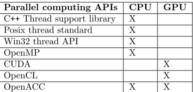
There are several different parallel computing Application Programming Intefaces (API) for expressing concurrency for CPUs and GPUs; a list of common programming models for parallel programming compatible with C++ is shown in Table3.

Parallel computing APIs CPU GPU C++ Thread support library X

Posix thread standard X

Win32 thread API X

OpenMP X

CUDA X

OpenCL X

OpenACC X X

Table 3: Examples of parallel computing APIs for expressing concurrency in C++

C++ Thread Support Library is a threading library available in the C++11 standard library [19] and allows developers to express concurrency through threads. Posix thread standard and Win32 thread API are similar to the C++11 thread library although with the drawback of being platform dependant to Unix and Windows respectively [20]. These parallel computing APIs are suitable to perform asynchronous tasks such as I/O and GUI updates that runs in the background of the main program [4].

Compiler directed parallelism such as OpenMP [21] is also a programming model to express concurrency on the CPU, however, it differs compared to the previously mentioned threading libraries in the way concurrency is expressed. The benefit of OpenMP is that the sequential code will not have to change in many cases and if the compiler do not support it, the directives will simply be ignored.

(9)

When it comes to parallelizing GPUs there are additional things to consider in comparison to CPU parallelization. One of the factors limiting potential speedup from parallelization on GPUs compared to CPUs, is that the GPUs usually do not share the same memory space as the CPU. This means that the data required for computations needs to be transferred to the GPU before starting the computations. In addition to this, the results must then be transferred back from the GPU to the CPU memory space. This introduces an additional overhead for parallelization on GPUs and may therefore limit the benefits of utilizing them.

CUDA is the parallel computing API invented by Nvidia which enables the developer to utilize the GPU for general purpose computations. Introduced in 2006, CUDA is a general purpose par-allel computing platform as well as a programming model for Nvidia GPUs. The compiler NVCC, also developed by Nvidia, is used to build code for the GPU using CUDA. The CUDA code is built by NVCC while the CPU code, or host code in CUDA terms, is built by a compiler of choice such as the VC++ or GCC compilers [22].

Open Computing Language (OpenCL) is an open standard maintained by The Khronos Group [23]. Similar to CUDA it can be used to express parallelism on a GPU, however, OpenCL is not bound to a specific platform. Instead, OpenCL is a cross platform language able to express paral-lelism on both AMD and Nvidia GPUs as well as other platforms such as FPGAs.

OpenACC is another parallel computing API that utilizes compiler directives similar to OpenMP in order to express concurrency. OpenACC differs from the other approaches since it supports both CPU and GPU acceleration, allowing for a very portable code.

(10)

4 Related Work and Comparison to our Contribution

There has been much research within the field of parallel computation over the years. Since the contribution of this work is a method to re-engineering sequential software to introduce paral-lelization, the studied related work focuses on other development approaches or methodologies for parallel software rather than programming guides or generic software development methods.

In 2003 Intel [18] presented a method to introduce threading in sequential software using a generic development lifecycle consisting of six different phases. These phases are 1. Analysis, 2. Design, 3. Implementation, 4. Debugging, 5. Testing and 6. Tuning. The lifecycle is of a waterfall [24] nature with the exception of debugging, testing and tuning. These steps are intended to be performed iteratively until errors are found and fixed. The drawback of their method is that it targets developers using Intel threading tools only to introduce parallelization. Additionally, the parallelization is only considered for CPUs which limits the hardware utilization in systems con-taining both CPUs and GPUs.

The work presented by Tovinkere [16] is greatly similar to the approach presented by Intel 2003. The development lifecycle is also a general development lifecycle that has six different phases, al-though they differ slightly compared to the one in [18]. The steps in their method are as follows: 1. Analysis and Design, 2. Implementation, 3. Debugging, 4. Performance Tuning, 5. Re-mapping and 6. Unit Testing. Similar to the method presented in [18], the goal is to utilize threading to increase the performance of software. In comparison to Intel’s method [18], Tovinkere’s is more specific to parallel software development whereas Intel’s follows a general software development method. Tovinkere’s approach is less tool-dependent, although when applying it to a specific case they suggest Intel tools too. Both methods are specific to threading on CPUs and only consider the technical aspects of the development.

Jun-feng [20] provides an approach that consists of seven different steps, in which some of them also consist of several substeps. Their model is following a waterfall development cycle. During the initial phase of the development cycle they briefly mention financial costs in the form of hardware investment as well as development cost. The approach does not consider locating parallel potential in any way and initially assumes that there is code to perform a feasibility analysis on. Their model is also limited to parallelization on CPUs.

Christmann et al. [25] present a method for porting existing sequential software to a paral-lel platform. Their method takes into account financial aspects of the development costs of the parallelization of the existing software. Their approach consists of four different phases which are preparation, analysis, implementation and adaption. In their study the method is applied on a smaller program for evaluation, however, their results suggest that the method is more suitable for bigger programs.

The method proposed by [26] is based upon an iterative approach they call Assess, Parallelize, Optimize, Deploy (APOD). The idea behind this approach is to be able to deploy a parallelized portion as soon as possible to quickly create value for the users. In contrast to previously men-tioned related works, this methodology considers parallelization on GPUs. However, this is also one of the drawbacks with their approach since it only targets parallelization on the GPUs.

The method presented in [27] proposes an iterative approach to introducing parallelization to legacy software. Their iterative process contains five different steps: Save current version, change, check new version, accept or reject and finally document. To introduce parallelization in to legacy Fortran software they propose the use of OpenMP and only consider CPU parallelization.

(11)

One of the major differences of the methods presented by [18, 16, 20, 26, 27] in comparison to ours is the consideration of effort estimation for the parallelization. During the analysis our method includes an effort estimation for the parallelization, which is further described in Section

6.2. This gives the opportunity to prioritize parallel potential portions of the software with higher speedup potential. This can potentially mean that a higher speedup can be achieved within a set budget of development effort. On the other hand, our parallelization method therefore introduces a slight extra overhead work to do this estimation. However, not taking this into consideration can potentially result in spending effort on less valuable parallelization potential regions. At the same time for our method, the extra overhead may be introduced for parallel potential regions that are not implemented in the worst case scenario. Because of this extra overhead, our method is potentially better suited for larger existing software codebases where this overhead would represent a smaller fraction of the total parallelization effort.

Another difference between the method presented by [18,16,20,25,26,27] is that our method considers both CPU and GPU parallelization and theirs considers parallelization on either CPUs or GPUs only. Additionally, the method proposed by [26] is specific to CUDA enabled hardware while the methods proposed by [18, 16] targets Intel hardware and tools. This would also mean that the hardware is under-utilized if these methods are used in systems where both CPUs and GPUs are available. Instead, the method we propose is more generic and does not limit itself to specific hardware or tools and considers parallelization on CPUs and GPUs. However, since their methods are specific to certain hardware and tools, they are able to give more advice regarding implementation, potentially yielding more effective speedup on the specific hardware they are lim-ited to when the suggested tools are available.

While there exists several different methodologies to the development of parallel software, there is still a risk of under-utilization of the available hardware since they do not consider parallelization on both CPUs and GPUs. Besides this, there is also a risk of the development cost running out of control if financial aspects of the development are not considered. Therefore, there is a need to consider technical aspects of parallelization, meant as utilizing both CPU and GPU, as well as the financial aspects of this parallelization process. This work addresses these two points.

(12)

5 Research Method

In this study the methodology used in order to approach the problem was the engineering design process [28], defined by the following seven steps:

1. ”Define the Problem” 2. ”Do Background Research” 3. ”Specify Requirements” 4. ”Create Alternative Solutions” 5. ”Choose the Best Solution” 6. ”Develop the Solution” 7. ”Test and Redesign”

Before the work could start, the first step was defining the problem that needed to be solved. In order to tackle the problem described in Section2the goal of this study was to define a method for introducing parallelization to existing software.

With this goal in mind, the next step of the process was to do background research regarding state-of-the-art solutions to similar problems in order to gain knowledge of existing methods for parallelizing sequential software. This was achieved through an informal literature review searching relevant databases such as IEEE, ACM, Springer and Google Scholar [29, 30, 31, 32]. These databases were chosen because they include publications within the topic of computer science and the availability for the author. The purpose of this literature review was to gain knowledge on the following:

• Existing methods for parallel software development • Introducing parallelization to existing software • Localization of parallel potential in software

• Utilization of CPU and GPU for parallelization of software

With this in mind, keywords such as ”Parallel Software”, ”Parallelization”, ”Software engi-neering method”, ”Multi-core CPU” and ”GPU” were used. Papers were selected based on their relation to the topic of parallel software development and engineering. Although this study focus on the introduction of parallelization into existing software, literature focusing on the development of parallel software was included. This was because literature focusing only on parallelization of existing software was limited. An analysis and comparison of the existing parallelization methods was performed in order to find their strengths and weaknesses. This was done by performing a Strengths, Weaknesses, Opportunities and Threat (SWOT) analysis [33].

The next step was to specify the requirements of the parallelization method. The identified strengths and weaknesses of existing methods were summarized and analyzed. Requirements were defined with the goal to inherit these strengths and at the same time avoid introducing the weak-nesses to the method. These requirements along with the initial goals of the study was combined into the requirements specification for the parallelization method.

The design of the parallelization method was started and the creation of alternative solutions was done by sketching down different ideas for a solution, based on the requirements defined in the previous step. Alternative methods was divided into different configurations of steps and phases. Once an idea for a solution was created, it was analyzed for strengths and weaknesses. In the end, the choice was between two fairly similar options but with one difference, further discussed in Section 8. Once one of these solutions were selected as the best solution it was taken to the

(13)

development phase, as described in Section6.

Once the parallelization method was defined, the next step was to test and evaluate it. In several of the related works the evaluation was done by applying their method on smaller pro-grams or in experimental environments [25,34]. The drawback with doing this is that conclusions cannot be drawn for how the method performs when applied to larger systems in a real world environment. Instead, in this study the parallelization method was evaluated by applying it to an existing real-life industrial system. The details of the design of this process is described in Section7. Additionally, the developed method was also compared to existing methods. The data collected from the SWOT analysis of the state-of-the-art was compared to the data retrieved from the experiment in order to evaluate our parallelization method. This was done in order to show benefits and drawbacks of the derived parallelization method. This comparison is described in Section 4 and can be used to decide which parallelization method fits better on a case-by-case basis.

(14)

6 Results

In this section we present the thesis contribution. Section6.1starts with an analysis of the existing parallelization methods. Based on this analysis a set of requirements followed by the definition of the parallelization method is presented in Section6.2.

6.1 Analysis of existing methods for parallelization

In this section we present existing parallelization methods as well as a SWOT analysis on each of them. This was done with the purpose of finding their strengths and weaknesses in order to refine the requirements for the parallelization method presented in this study.

As mentioned in Section 3, Intel presented a development method to introduce threading in software to increase performance in 2003 [18]. The Strength with this method is that the devel-opment methodology is simple to understand. However, it has a structure similar to the waterfall model [35] and therefore inherits its weaknesses. One notable Weakness of the method is that changes to requirement or discovering errors late in the development can be very costly [24]. In addition to this, the method targets users of specific hardware and tools (Intel processor and tools) only. Although, in the case where the specific hardware and tools are available, the methodology provides Opportunities to achieve better performance. At the same time, it does not consider uti-lizing ways of introducing parallelization other than through threading on CPUs, therefore there may be cases where this method does not utilize the full potential of the hardware which could be seen as a Threat.

In the method presented by Tovinkere [16] the Strength is that it is more specific to parallel soft-ware development in comparison to [18], but still remains simple to understand. The Weakness of this method is also that it targets specific hardware and tools only. Moreover, it does not consider financial aspects in terms of development costs of introducing parallelization into software. There is an Opportunity to fully utilize suggested tools to gain optimal performance from the software. Since the method only applies to specific tools and hardware, there is a Threat that the software lacks in portability. In addition to this, the method does not consider GPU parallelization which can potentially limit the performance gains.

In [20] the authors present a method whose Strength is that it takes the feasibility of a par-allelization of a piece of software into account. On the other hand, its Weakness is that it does not consider locating parallel potential nor validating the software after the parallelization. Addi-tionally, it only considers parallelization on CPUs. The Opportunity is that, due to the fact that the method only focuses on technical aspects of the parallelization it produces low overhead. The Threat with using this method is that the software may contain errors since software testing is not considered as part of the method.

Christmann et al.’s methodology [25] has the Strength that it considers the financial aspects of developing software. The Weakness of the method is that it does not consider GPU usage for parallel computation. An Opportunity due to the fact that this method considers financial aspects of development is that the costs can be kept under control. On the other hand, this also introduces additional overhead which may be seen as a Threat in cases where the overhead outweighs this benefit.

The Strength with the method proposed by Nvidia [26] is that it uses an iterative approach to development which allows for continuous deployment and considers the use of GPUs for par-allelization. The Weakness is that it does not consider financial aspects nor utilization of CPUs and instead focuses only on optimization on GPUs. In addition to this, the method is also limited to parallelization on CUDA-enabled devices. The Opportunity with this approach is that since GPUs carry much computational power the potential for greater performance increases compared to limiting the parallelization to CPUs. Because the method is limited to GPUs, as well as limiting itself to CUDA enabled GPUs, its target audience is severely limited which poses a Threat when

(15)

the software needs to be available on multiple platforms with different hardware configurations. In [27] the authors present a method whose Strength is that the iterative method focuses on managing changes to already working software without breaking it. The Weakness of the method is that it is limited to Fortran code and the use of OpenMP, meaning that a GPU would not be utilized if available. However, the Opportunity is that speedup may be achieved while maintaining the validity of the software, if the legacy is written in Fortran. Since parallelization on GPUs are not considered, there is a Threat that the hardware may be under-utilized.

A summary of some strengths and weaknesses identified in existing methods from the SWOT analysis is shown in Table4

Strengths Weaknesses

Simple to understand Waterfall model Feasibility analysis Targeting specific tools

Considers financial aspects No parallelization on both CPUs and GPUs Iterative process No validation

No parallelization potential localization Table 4: Located parallel potential locations

From the results of this analysis it is clear that only one of the analyzed methods considers financial aspects in terms of additional development costs that parallelization introduces. Consid-ering that developing parallel software is a more complex task than to develop sequential software [4], there is a risk that the parallelization of sequential software comes with a high cost. Effort of introducing parallelization is therefore an important consideration in order to keep the costs under control. In addition to financial aspects, the use of the GPU for parallel computation is also considered by one method only. At the same time there is no method that considers both parallelization on CPUs and GPUs together.

6.2 Definition of the parallelization method

Based on the analysis in the previous section the following set of requirements on the parallelization method was defined. The method should:

1. Consider the use of both CPUs and GPUs for parallelization 2. Consider effort required to parallelize sequential software 3. Include validation of the parallelized software

4. Provide an iterative development process 5. Not target specific tools

1. and 2. are direct consequences of the aforementioned research challenges and represent the novelty of this contributions since, as shown in the previous section, no existing approach provides both. 3. Validating that the parallelization does not introduce errors or unexpected behaviours must be part of the parallelization method, since it is instrumental in any software engineering process. 4. The parallelization method should provide an iterative development approach to incrementally parallelize software portions and continuously validate results. Additionally, this could also allow for continuous integration and deployment. 5. The parallelization method should not target specific tools, in order to be applicable by an as broad audience as possible.

(16)

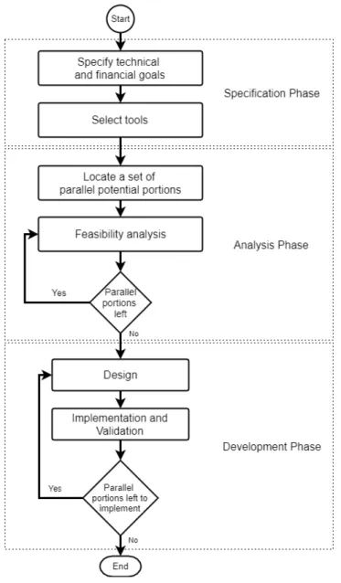
The parallelization method that we propose consists of three different phases and is depicted in Figure2. The first phase represents the defintion of the goals of the parallelization as well as the tools to use. In the second one, the analysis phase, developers analyze the software for parallel potential and perform a feasibility analysis. The last phase is the development phase, where the feasible portions of the software are further analyzed and a parallel solution is designed, imple-mented and validated.

Figure 2: Parallelization method

In the following subsections a more detailed description of the phases is presented. 6.2.1 Specification phase

In this phase, the engineer specifies the goals of the parallelization and decides which tools to use. As shown in Figure2, the first step is to decide what the goals of the parallelization are. The goals can be divided into two categories, financial and technical goals. In this method the financial goals are expressed in terms of development effort introduced by the parallelization. However, there are cases where not only the parallelization of the software itself affects the costs. For example, in some cases the parallelization may introduce increased costs in terms of energy consumption. In cases where such aspects are vital, these other forms of financial aspects and how they affect the

(17)

parallelization process must also be taken into consideration.

Technical goals can be expressed in terms of desired speedup as result of the parallelization. According to [25] there are two different approaches to choose between: one is to prioritize the cost before the performance while the other is to prioritize the performance above the cost. The first approach can be described as parallelizing a piece of software as much as possible within a certain budget, e.g. the development cost. Once this budget is used the parallelization stops no matter how much the performance has improved. The other is to set a target level of performance that the software needs to reach. The parallelization is carried on until this target is reached. In many cases the first option may be preferred since a ”good enough” solution is more likely to be more cost effective. However, in some cases where there are timing restrictions that require a certain level of performance, the second option may be needed.

The next step is to specify what kind of tools to use for the parallelization. This step is very dependent on what the existing software’s characteristics are. For example, if the existing software is written in C++, then tools that support C++ have to be used. Although, if it would be beneficial to first modify the existing software in order for it to be used on a specific unsupported tool, it is recommended to do so. However, this will have to be decided on a case to case basis and is not covered by this work. One type of tools that should be chosen during this step is a profiling tool, to be used during the next phase to aid with parallel potential location. In addition to this, a timer to measure the execution time of portions of the software will be used for the feasibility analysis in the next phase. Additionally, in this phase the engineer selects which parallel computing APIs to use. This decision is also affected by the existing software, for example which platform it is intended for, used programming language and compiler. Since our method is meant to be generic and applicable to a wide variety of existing software, this choice also needs to be taken on a case to case basis.

6.2.2 Analysis phase

The purpose of this phase is to analyze the software to find potential for parallelization. Two tech-niques can be used to perform this task: manual and dynamic analysis of the software. In some cases, the parallelization is not necessarily performed by someone that has an in depth knowledge of the details of the complete software. In such cases it can be beneficial to perform additional manual analysis of the software to gain a deeper program understanding. Analyzing the control flow of the software can give additional program knowledge as well as revealing task-parallelism potential in the program flow. Manual inspection of the software can be a time consuming task, therefore, using dynamic analysis can help to point out where in the software to look for parallel potential. A profiling tool can be used to search for pieces of the software where much of the execution time is spent, i.e. hot-spots. The idea behind searching for hot-spots is that if these portions of the software are parallelized, the total gain of performance is greater than parallelizing a portion that is rarely used. Once this analysis is done and a set of hot-spots is defined, a manual inspection of the code should be performed. This is done with the purpose of deciding whether there is any potential for parallelization in that piece of software. Parallel potential is found by looking for computations that are not dependant of each other and can therefore be performed in parallel.

When locations for parallel potential have been found, it is time to do a feasibility analysis on them. The purpose of this is to find out if it is worth performing the parallelization on the piece of software. The first step is to evaluate how much of the code can be parallelized. Once this is defined, an estimation of the potential theoretical speedup from parallelization can be calculated by using Amdahl’s law or Gustafson’s law, as described in Section 3. Since these laws expect a number of processors to apply the parallelization on, a decision of whether to utilize CPUs or GPUs for the parallelization must be taken.

(18)

To decide whether CPUs or GPUs (or both) shall be employed, we first need to check whether a task-parallel or data-parallel approach is more appropriate. In the case where a task-parallel approach is selected, then CPUs are used for the parallelization. By considering the number of processors of the target hardware when applying Amdahl’s or Gustafson’s law we can estimate the potential speedup from parallelization.

On the other hand, if we decide to go for data-parallel approach, an estimation of the potential speedup in case of CPUs or GPUs must be done in order to choose between them. Apply Ahmdal’s or Gustafson’s law first targeting a CPU and then a GPU. Characteristics of the GPU, such as clock frequency and memory clock frequency, may differ from those of the CPU, this must be taken into consideration when analysing the results of speedup estimation. In addition to this, the grain-size of the parallel task plays a role in the selection of the processing unit type too. Since GPUs often have several hundreds and in some cases even thousands of cores, the parallel task should be fine-grained enough to utilize these cores. If the task is coarse-grained and unable to utilize the available cores, the GPU would be under-utilized; then it would be better to use a CPU instead. If the task is suitable for both CPU and the GPU, the results from the speedup analysis decide of whether to utilize the CPU or the GPU.

The second step of the analysis phase is to estimate how much it will cost to go through with the parallelization. There are three things that needs to be estimated: the time to design a paral-lel implementation, the time to implement the paralparal-lelization and to validate the paralparal-lelization. First, analyze the code size and complexity and estimate how much time it will take to design a parallel implementation. Next, analyze the code to see if there is a need for refactoring the existing sequential code in order to go ahead with the parallelization. Estimate the time it would take to refactor the code (if necessary) and implement a parallel implementation. The final step is to estimate how much effort the validation will take. Once these estimations are made they can be combined into a total estimation of the required effort to design, implement and validate the parallel potential piece of software.

When these two values are defined for a piece of software they can be combined to see how fea-sible it is for parallelization. If the potential gain is very small and at the same time the estimated cost is high, a decision must be taken whether it is worth even attempting to parallelize it or not. There can even be cases where the overhead introduced by the parallelization is greater than the performance gain, in this case the resulting software would turn out to be slower than the original. In this case, the choice to not parallelize this piece of software should be taken.

Once the feasibility analysis has been applied to all located parallel potential locations, it is time to prioritize them according to the available budget.

6.2.3 Development phase

This is the last phase of the parallelization method and it is performed iteratively. The following steps are applied to all chosen pieces of software selected for parallelization starting with the one set to the highest priority.

The first step of the development phase is to design how the selected piece of software should be parallelized. In the analysis phase an initial design decision was taken regarding which hardware platform to utilize. If the chosen hardware was the CPU the problem is either of a task-parallel or data-parallel nature. In the case of a task-parallel problem it is recommended to use a threading library such as the C++ Thread Support Library [18,16,36]. On the the other hand, when it comes to parallelize data-parallel problems on the CPU, the recommendation is to utilize a compiler directed approach such as OpenMP [18,16,20,26]. If the chosen compiler does not support such a technology, a threading library can be used as an alternative. If the chosen approach was to utilize the GPU for the parallelization, we can simply use the parallel computing API selected in the specification phase.

(19)

Additionally, the piece of software selected for parallelization must be further analyzed in order to design the implementation of the parallelization. In some cases refactoring of data may be necessary in order to allow for better parallelization.

The implementation and validation step of the process was decided to be combined into one step. The implementation approach is freely chosen by the engineer since it does not affect the expected gains.

(20)

7 Evaluation

In order to evaluate our parallelization method, we set up an experiment exploiting a real-life in-dustrial software system. The results from this evaluation were then used to compare the method to the other existing parallelization methods as described in Section4. The goal of the experiment was to apply the parallelization method on an existing sequential software to introduce paralleliza-tion, as a proof-of-concept.

At ABB Robotics a topic that is considered quite extensively at the moment is 3D sensors and what they can bring regarding awareness of the environment for the robots. 3D sensors using structured light have opened up new possibilities for robotics and the provided 3D data can be used to describe a robot’s surroundings in more detail. That is, this kind of sensor can be used when scanning an environment in order to determine collision free paths in the 3D space. This effort has been going on for some time and sequential software has been developed yielding good performance regarding perception. The problem is that the execution time is too high and that today’s single computer cores are inadequate for the task. In addition to this, today’s 3D sensors don’t have any additional processing capabilities for vision algorithms, making the data acquisition slow. Therefore, to be able to obtain real-time behaviour of a 3D vision system, a processing device with higher computational power must be placed near the vision sensor. As previously mentioned in Section3, GPUs are designed for highly parallel computation and leading graphic card vendors are currently offering small circuit boards with integrated processors and GPUs targeted to embed-ded environments [37,38]. However, to run the existing software on such a platform, it needs to be re-engineered in order to introduce parallelization and thereby exploit the potential of parallel hardware.

In order to know what kind of data had to be collected during this experiment, a set of research questions was defined as follows:

1. How much overhead does the parallelization method introduce?

2. How much did the execution time of the parallelized software improve from the original? 3. Are there any limitations in using the parallelization method?

Data was collected in multiple ways, combining quantitative and qualitative measurements. In order to answer the first research question, the effort spent on each step of the approach was recorded with the purpose of tracking how much time is spent on preparation and planning com-pared to the actual implementation of the parallelization itself. Benchmarks was performed on the chosen pieces of software for parallelization before and after the parallelization method was applied. The data recorded from these benchmarks was used in order to answer the second re-search question. Additionally, we evaluated the parallelization method after the experiment with the purpose of collecting qualitative data. This was done in order to gain an understanding of how the experience of using the parallelization method was perceived by those applying it, with the goal of answering the third research question.

7.1 Experiment

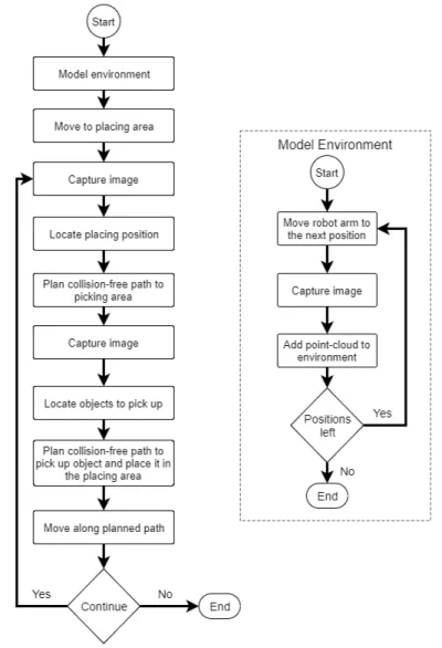
The experiment was carried out at ABB Robotics. The parallelization method was applied on a palletizer application that is developed as a proof-of-concept for a 3D vision library at ABB Robotics. The application is quite simple in itself and the objective is to use a robot arm to pick and place objects from point A to point B. In this particular application the exact location of point B is unknown beforehand and only a larger area of where B’s location is, is known. The same goes for the location of the objects, whose exact position is unknown. In order to identify the location of the placing area (point B) as well as position and orientation of the objects to be moved, the application uses the 3D vision library. The control flow of the application is shown in Figure3.

The first thing to do before the application can start using the robot arm to pick and place items is to model the static environment around itself using a 3D camera that uses structured light. The robot arm moves around and captures multiple images from different angles around itself and

(21)

Figure 3: Control flow of the Palletizer application

stitches the images together. The static environment is then stored as a point-cloud [39] in the coordinate system of the robots base. Now that the static environment is modeled and stored, the first step of the main loop is to move to the general area where the placing area is and capture an image with the 3D camera. Using the stored model of the environment, everything except the placing area can be extracted from the point-cloud using a background extraction algorithm from the 3D vision library. The application is now aware of the exact location of the placing area and can move the robot arm to the picking area. An image is captured once the robot arm is above the picking area in order to locate objects to pick and place. The static environment can be extracted from the captured 3D image, in the same manner as it was done for the placing area, in order to remove everything except replaceable objects. The application now uses a 3D model in the form of a point-cloud to represent objects and locates them using another algorithm from the 3D library, which gives the objects location and alignment. Once the location and angle by which the robot should pick up the object have been identified, the robot arm can pick the object up and place it in the desired alignment on the placing area. This loop can now be repeated in order to pick and place the remaining objects.

(22)

The issue with this sequential application is that the vision algorithms are very computational heavy. Once an image is taken, the application needs to wait for the algorithms to finish before it can move the robot arm again. This idle time increases the cycle time of the program and therefore the throughput is low. Our experiment consisted in applying our parallelization method to this application in order to increase its overall performance. In the following subsections the application of the parallelization method is described.

7.1.1 Specification phase

To specify the goals of the parallelization, a speedup maximization approach was used, meaning that the goal was to maximize the speedup within a given budget. The budget for the paralleliza-tion is specified in terms of time representing development effort. The budget for the development was set to five weeks of 40 hours each week, giving a total development time budget of 200 man hours. Besides maximizing speed-up, an additional goal was to make the parallelized software runnable also on platforms not including GPUs. This means that if the parallelization of a func-tion was implemented on a GPU, the same funcfunc-tion should also be parallelized on a CPU in order for the parallelization to yield speedup on platforms of different kinds. Additionally, this would allow a comparison between the results from parallelization on CPUs and GPUs in terms of devel-opment effort and achieved speedup. The decision between which implementation to use is taken at runtime depending on the platform configuration.

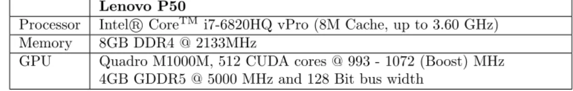
The development as well as the benchmarking was carried out using a Lenovo P50 laptop with Windows 7 as operating system. The specification of the hardware of the computer is specified in Table5.

Lenovo P50

Processor Intel CoreR TM i7-6820HQ vPro (8M Cache, up to 3.60 GHz) Memory 8GB DDR4 @ 2133MHz

GPU Quadro M1000M, 512 CUDA cores @ 993 - 1072 (Boost) MHz 4GB GDDR5 @ 5000 MHz and 128 Bit bus width

Table 5: Development and benchmarking hardware

The existing code base was developed using Visual Studio 2015 (v140 platform toolset) and Microsofts VC++ compiler and the code was compiled using the -O2 optimization flag. The C++11 threading library and OpenMP was used in order to express concurrency on the CPU when applying the parallelization method. This was decided since the existing codebase was already using the C++ standard library and the compiler also supports OpenMP. The intention was to use C++11 threading library to express task-parallelism while OpenMP for data-parallel tasks. In order to express concurrency on the GPU, we used CUDA. This decision was based on the fact that the target system includes a CUDA enabled GPU. Time spent in this phase was 8 hours.

7.1.2 Analysis phase

As shown in Figure2, the first step of the analysis phase is to locate a set of software pieces that could potentially be parallelized. In this experiment, the first step was performed through both a manual control flow analysis of the application and a dynamic analysis. The manual analysis was done to get a better understanding of how the application worked and to locate parallelization potential in the program flow. A high-level control flow of the application is depicted in Figure

3. Based on the control flow and dependencies between the actions, there were two visible lo-cations for parallelization. The first one is in the environment modeling procedure, where there is no dependency between moving the robot and adding the point-cloud from the image to the point-cloud representing the environment. There is therefore potential for parallelization in this case, where the robot could move to the next position at the same time as the application models the environment. The second one is when a picture is taken of the placing area and the placing position is calculated, after which a collision free path is planned to the picking area. This path planning is not dependant of the result of the placing area image results, and so the actions could

(23)

actually be run in parallel.

In addition to the manual control flow analysis, a dynamic analysis was performed using Vi-sual Studio Profiling Tools with the intention to find hot-spots in the code. The result of this analysis showed that many of the hot-spots were located inside third party libraries used by the software. However, since the goal was not to parallelize the third party libraries, the hot-spots located outside the target software were ignored. The result showed 13 functions, apart from the third-party functionality, that were accessed frequently and consumed much computational power. These functions were then inspected and analyzed manually for parallelization potential. After the analysis, 6 functions were identified as parallelizable. Table6summarises the located software portions with parallelization potential.

Parallel potential Location method Model environment Manual analysis Locate placing area Manual analysis Extract environment Dynamic profiling Align object Dynamic profiling Edge detection Dynamic profiling Stitch point-cloud Dynamic profiling Table 6: Located parallel potential locations

Once these locations of parallel potential software were located, we conducted a feasibility anal-ysis on them to check whether they were actually parallelized.

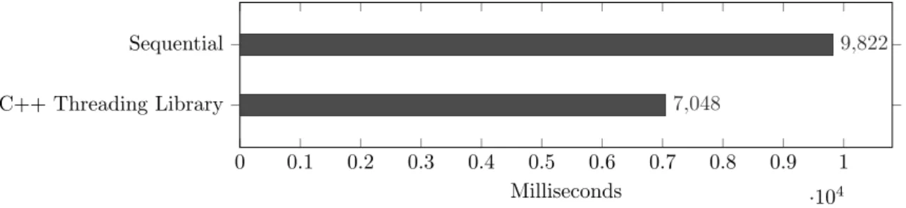
Modeling the environment was the first potential location for paralellization and was found through the manual analysis of the software. This part of the code takes care of combining multiple images taken from the robot arms perspective. As shown in Figure3, the robot arm moves to a set of positions and takes an image at each position. In this case, the potential for parallelism here is to add the previously taken image to the environment at the same time as moving the robot arm to the next position. The parallelization of this function would run on two parallel cores. This is because there are only two task that can run in parallel, meaning that it cannot scale to additional threads. In order to estimate the potential speedup achievable through parallelization, we used the following procedure: First, the total time it took to model the environment was measured. The total execution time for this was measured to 9822 millisecond. Then, the individual times of the two tasks that could run in parallel was measured. For adding new point-clouds to the environment this was measured to 2816 milliseconds while moving the robot arm was measured to 6635 milliseconds. The remaining 371 milliseconds was spent on communication with the image sensor and the robot controller, which needed to be performed sequentially. Since adding images to the environment can be performed in parallel to moving the robot arm which is a longer process. Meaning that in theory, 5632 milliseconds (2*2816) of the sequential execution time could run on different cores at the same time. This is 57.34% of the total execution time. The results of applying these numbers into Amdahl’s law is shown in Equation4.

Speedup(2)Amdahls0_s=

1

(1 − 0.5734) + 0.5734/2= 1.4 (4) While the estimated speedup factor of 1.4 may not seem large, the execution time of modeling the environment is measured to 9822 milliseconds in total. In Equation5 we apply this speedup factor to the measured execution time to estimate what the speedup would translate to in terms of time.

9822

1.4 = 7015.71 (5)

The result from this speedup estimation suggests that if this theoretical speedup could be achieved through parallelization, the execution time would be 2806.29 milliseconds faster than the

(24)

sequential code.

Locating the placing area was also found as a potential location for parallelization through manual analysis. In this case there were two different tasks performed sequentially that were not depending on each other: locating the placing area and calculating a collision free path to the picking area. The total execution time for these two tasks were 2205 milliseconds. Individually the tasks measured at 493 milliseconds for locating the placing area and 1712 for calculating the path to the picking area. It is therefore estimated that 44.72% of the code can run in parallel since 986 milliseconds (493*2) of the execution time can run on two separate cores. Equation6 shows the potential speedup factor from applying these numbers using Amdahl’s law.

1

(1 − 0.4472) + 0.4472/2 = 1.29 (6) The estimated speedup factor achievable through parallelization was 1.29. In order to under-stand what this potential speedup translates to in terms of time, we applied these numbers in Equation7.

2205

1.29 = 1709.3 (7)

These results also show a fair potential for speedup in terms of time. Since the total execution time is 2205 milliseconds, a parallelization that achieves this speedup would reduce the execution time by 495.3 milliseconds.

Extracting the environment from an image was another software piece with potential for paral-lelization. The sequential execution time of this function was measured to 295.4 milliseconds. An analysis of this piece of software showed that it contained code that could potentially cause race conditions if executed in parallel, by reading and writing to the output of the function. This code must therefore run sequentially in order to avoid corrupting the output. Additionally the execution time of this was measured to 4.14 milliseconds. Additionally, computations performed on the code that needs to run sequentially was measured at 4.14 milliseconds while the parallelizable portion of the function takes 291.26 milliseconds. This means that 98.6% of the execution time can run in parallel. The next step was to decide which parallelization approach to use. To do that, we first needed to classify the problem as task-parallel or data-parallel. In this case, the problem was classified as data-parallel because in order to extract the static environment from a point-cloud, the algorithm checks for every point in the point-cloud whether it exists in the environment or not. At this point, the speedup estimation was performed for both CPUs and GPUs according to the parallelization method. Equations8 and9shows the results when applying these numbers to Amdahl’s law. Speedup(4)Amdahls0_s= 1 (1 − 0.986) + 0.986/4= 3.83 (8) Speedup(512)Amdahls0_s= 1 (1 − 0.986) + 0.986/512= 62.79 (9) Note that the estimated speedup in Equation 9 is the theoretical speedup in the case when the sequential version is executed on the GPU. However, the GPU used in this experiment has a core frequency that is only 27.7% of the CPUs core frequency. The estimated speedup from parallelization using the GPU based on the difference in core frequency would be 16.5 (62.79 * 0.277). This means that in theory parallelizing it on the GPU would give a better speedup. Additionally, we analyzed the code to see how many computations may run in parallel to know if parallelization on GPUs is suitable. This analysis showed that 307200 (the size of the point-clouds) calculations can be performed in parallel, which means there are enough parallel computations for the 512 cores available on the hardware. For this specific experiment, as mentioned in Section

7.1.1, functionality should also be parallelized for a CPU in the case where a GPU parallelization approach is chosen.

(25)

Aligning object to find location and orientations of them inside a point-cloud was found as a location for parallel potential through dynamic analysis. Measuring this function showed an execution time of 1548.54 milliseconds. Similar to the previous piece of software, this function also contained code that had to run sequentially. The sequential portion of code was measured at 18.73 milliseconds and is therefore 1.2% of the whole execution time. This means that 98.8% of the code was parallelizable. Additionally, after analyzing this piece of software it was decided that a data-parallel approach was approapriate. The same action is taken for every data in the task of aligning a point-cloud in another and calculating the amount of points that matches. We estimated speedup by applying Amdahl’s law as shown in Equations10and11.

Speedup(4)Amdahls0_s= 1 (1 − 0.988) + 0.988/4= 3.86 (10) Speedup(512)Amdahls0_s= 1 (1 − 0.988) + 0.988/512= 71.79 (11) The speedup estimations shows that aligning an object in a point-cloud has a good potential for speedup through parallelization. While the number of computations that can run in parallel in this case depends on the size of the point-clouds provided as input, we decided that this is a suitable piece of software to parallelize using GPUs. This is because the number parallelizable compuations are usually in between 100000-500000. This would give the GPU in our benchmarking computer enough parallel work to utilize the available 512 cores. Additionally, even though the frequency of the GPU cores are only 27.7% of the CPUs core frequency, it is still estimated that the parallelization on GPUs would yield a better speedup.

Edge detection is used to locate edges in point-clouds. This functionality was measured and the execution time was 32.73 milliseconds. The reading and writing to the output was needed to occur sequentially and this was measured at 2.42 milliseconds. Meaning that 92.6% of the computations can be run in parallel. After further analysis, it was decided that this should be classified as a data-parallel problem, since the same action is performed for every point in a point-cloud to decide whether it is an edge point or not. However, the size of the point-clouds provided as input are usually around 200 points when used in this algorithm since the point-clouds are down-sampled. Since we have 512 cores at our disposal, more than half of those cores would have no computations to execute. This would mean that the GPU is severely under-utilized, therefore, the speedup estimation and parallelization should be done for CPUs and the result is shown in Equation12.

1

(1 − 0.926) + 0.926/4= 3.27 (12) From these results we can see that the potential speedup factor is 3.27 and makes this a good candidate for parallelization.

Stitch point-clouds is the process of combining two point-clouds into one and execution time was measured at 248.1 milliseconds. Further analysis of the code showed that the reading and writing data to the point-cloud had to run sequentially. This portion of the code was measured and the execution time was 54.09 milliseconds, meaning that 78.6% of the computations could run in parallel. Stitching point-clouds was also defined as a data-parallel problem since the same action is performed for all points in the point-clouds. These numbers were used in combination with Amdahl’s law in order to estimate the potential speedup, the results are shown in Equation13.

Speedup(4)Amdahls0_s= 1 (1 − 0.786) + 0.786/4= 2.44 (13) Speedup(4)Amdahls0_s= 1 (1 − 0.786) + 0.786/512 + 0.1= 4.64 (14) 24

(26)

The results from the estimated speedup shows a decent potential for parallelization. While Equation14 shows better potential for speedup for a GPU parallelization, the difference in the hardware must be taken into account. Since the frequency of the GPU cores are only 27.7% of the CPUs frequency in this experiment, we expect that the speedup achievable from parallelization on CPUs will be higher. Therefore, it was decided to perform the parallelization using a CPU.

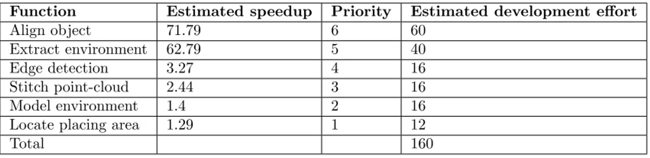
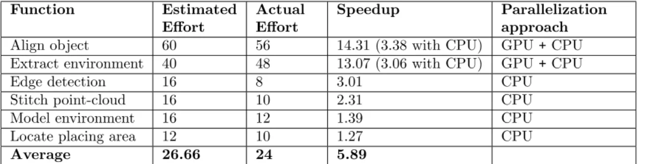
Now that the potential locations for parallelization have been located and analyzed, we can estimate the effort required for the actual parallelization and prioritize them in order to know which one to parallelize first. In this experiment we prioritized the parallel potential locations based on their estimated speedup estimation achievable through parallelization. The priority of the functions can be seen in Table7and they range from high to low where a lower number means a lower priority.

Function Estimated speedup Priority Estimated development effort

Align object 71.79 6 60

Extract environment 62.79 5 40

Edge detection 3.27 4 16

Stitch point-cloud 2.44 3 16

Model environment 1.4 2 16

Locate placing area 1.29 1 12

Total 160

Table 7: Priority and development effort estimation of parallel potential locations

After the specification phase and this analysis phase, the remaining budget in terms of man hours was 152. Based on this effort estimation, the effort (160) would exceed the remaining available budget (152). This means that the parallelization of the Modeling of the environment does not fit within the budget. However, it will still be kept as a planned parallelization in case it turns out that there is budget left when the implementation of the other parallel portions is completed.

7.1.3 Development phase

Once the analysis phase is completed, it is time for the parallelization development phase, which is done iteratively. More specifically, each step of this phase is performed on each included parallel potential location that fits within the financial budget starting from the highest priority.

Iteration 1

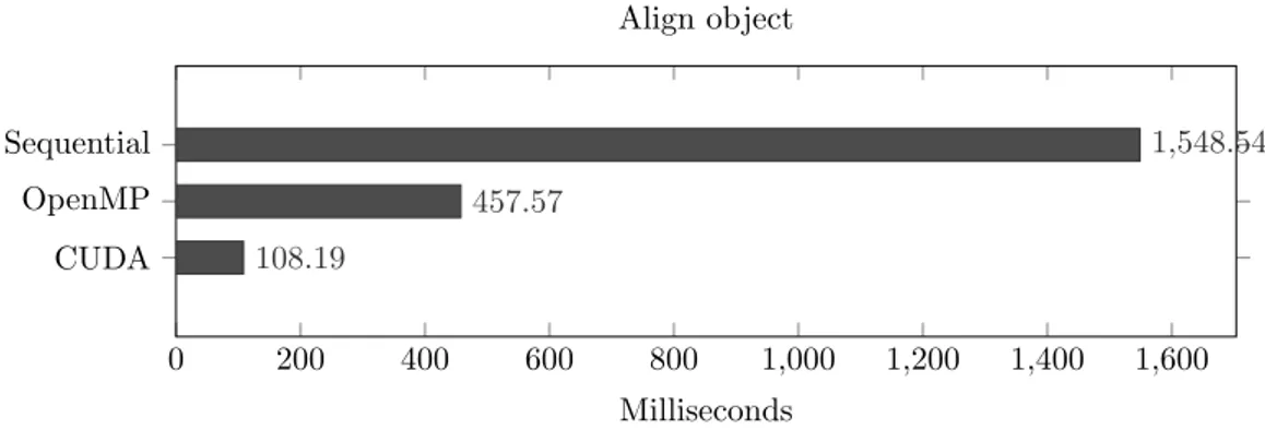
Based on the analysis in Section 7.1.2 the decision was to take a data-parallel approach using OpenMP and CUDA to parallelize the align object function. After further analysis of the code it was discovered that refactoring and implementation of several mathematical functions also had to be done for the GPU implementation. This was due to the use of third party libraries that were not callable from the CUDA code. This needed to be implemented in order to run the code using CUDA. Additionally, refactoring was needed to change some computation dependencies so that they could be performed in parallel. This resulted in the implementation taking more time than expected. The results of the parallelization are shown in Figure4.

This gives us the speedup by a factor of 3.38 for the OpenMP implementation and 14.31 on the CUDA implementation. The speedup of the GPU parallelization is mainly limited by the need to transfer data between the CPU and GPU memory spaces. The validation was done through the use of a unit test, comparing the expected result to the result of the parallelized implementations. Time spent on this iteration was as follows; 16 hours on analysis and design of the parallelization implementation, 40 hours were spent on the implementation and validation.

(27)

0 200 400 600 800 1,000 1,200 1,400 1,600 Sequential OpenMP CUDA 1,548.54 457.57 108.19 Milliseconds Align object

Figure 4: Execution times of Align Object after parallelization

Iteration 2

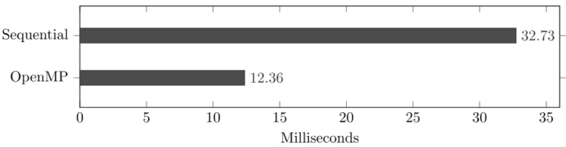
The next parallel potential location on the priority list is the functionality of extracting the envi-ronment from a point-cloud. From further analysis of this code a potential risk for race conditions was found, due to reading and writing to a list containing the output of the function. This was handled in different ways for the CPU and GPU implementations. For the CPU implementation a critical section was added to protect from multiple access to the list. As for the GPU implemen-tation, the decision was made to add an array of booleans representing whether a point should be kept or not. This allowed each thread on the GPU to read and write its result independently without interfering with other threads or corrupting any data. However, this also introduced a small overhead after the function since it required a sequential iteration through this array in order to add elements to the output.

After further analyzing the code, it was noted that this function also contained third party code that was not usable from CUDA code running on the GPU. Once this additional functionality was implemented, the implementation of the parallel version of extracting the environment was carried out for the CPU and the GPU. The result of this parallelization using OpenMP showed a speedup of 3.06 times compared to the sequential solution. As for the CUDA implementation, a 13.07 times faster execution time was recorded in comparison to the sequential one and 4.19 times faster than the OpenMP implementation as shown in Figure5.

0 50 100 150 200 250 300 CUDA OpenMP Sequential 22.6 96.47 295.4 Milliseconds

Figure 5: Execution times of Extract Environment after parallelization

In Figure 5 the difference in execution time is shown in milliseconds where the sequential so-lution takes 295.4 milliseconds while the parallel soso-lution takes 96.47 milliseconds. Additionally, the execution time of the CUDA accelerated implementation took 22.6 milliseconds. As previously mentioned this yielded a 13.07 times speedup which may not seem much considering the computa-tional capability of the GPU in the benchmarking system. However, this execution time includes the overhead from transferring the data to and from the GPU as well as the added overhead of sequentially iterating through the output. In order to validate that the parallelization did not introduce errors, a unit test was implemented to compare the expected output and the actual output from the parallel implementation.