Stuart L. Joy1 José L. Chávez2 Terry A. Howell3
ABSTRACT
Eddy covariance (EC) systems are being used to measure sensible heat (H) and latent heat (LE) fluxes in order to determine crop water use or crop evapotranspiration (ETc).
However, EC derived H and LE fluxes must be adjusted because EC systems systematically tend to underestimate actual H and LE heat fluxes. Thus, the energy balance does not close well generally for EC heat fluxes. A standard procedure for adjusting EC fluxes takes environmental conditions into consideration. This procedure allows for an improved determination of ETc values on an hourly and daily basis. The
objective of this study was to evaluate different adjustment methods and determine which one or combination of adjustment methods improved performance. For this purpose, two EC systems were installed near two large monolithic weighing lysimeters on irrigated cotton fields at the USDA-ARS Conservation and Production Research Laboratory at Bushland, Texas in the Texas High Plains during the months of July and August of 2008. A total of eight days (four in July and four in August) of EC data from two adjacent fields were post-processed and results were compared with the lysimetric ETc. The evaluation
included an analysis of the EC energy balance (EB) closure and residuals. Results indicated that the adjusted LE heat fluxes (converted to an equivalent amount of
evapotranspirated water depth) underestimated the measured ETc with an average error of
19-21% compared with 25-27% for the LE fluxes that were not adjusted. The residual errors occurred mostly during nocturnal measurements. The EB closure for the adjusted daytime fluxes was 88-97% which was an improvement over the 83-89% closure before adjustments. The EC frequency response adjustment had the largest impact in improving the EC-based ET values. This adjustment increased the LE fluxes by an average of 5.0-5.5%, and thus it was the most significant adjustment. Therefore we recommend that the combined adjustment method described be consistently applied when using EC to
properly measure ETc using EC systems for irrigated cotton in the Texas High Plains. INTRODUCTION
The methods or approaches by which crop or vegetation water use or evapotranspiration (ETc) can be measured are hydrological, meteorological, or based on plant physiology
1 Graduate Research Assistant, Department of Civil and Environmental Engineering, Colorado State
University, 1372 Campus Delivery, Fort Collins, CO 80523-1372; stuart.joy@colostate.edu
2 Assistant Professor, Department of Civil and Environmental Engineering, Colorado State University,
1372 Campus Delivery, Fort Collins, CO 80523-1372; jose.chavez@colostate.edu
3 Research Leader, Soil and Water Management Unit, Conservation and Production Research Laboratory,
Agricultural Research Service, U.S. Department of Agriculture, P.O. Drawer 10, Bushland, TX, 79012; terry.howell@ars.usda.gov
(Rose and Sharma, 1984). The hydrological approach is an indirect method in which ETc
is calculated as the residual of the soil water balance. For instance, lysimeters were used to measure water mass loss (therefore crop/soil ET) with high accuracy, according to Howell et al., (1995). However, lysimeters give only a single point measurement of ETc
due to its spatial limitations and cannot be easily moved to another location due to its large size and installation nature. The micrometeorological approach is a direct method in which ETc is a function of climatic variables. The eddy covariance (EC) method is a
micrometeorological approach based on the direct measurements of the product of vertical wind velocity fluctuations (w’) and a scalar concentration fluctuation (c’), like water vapor or air temperature, producing latent (LE) [Eq. (1)] and sensible heat (H) [Eq. (2)] fluxes, respectively, assuming the mean vertical velocity is negligible:
(1) (2) where LE and H are the latent and sensible heat fluxes (W m-2), w′ is the covariance q′ between fluctuations of vertical wind velocity, w’ (m s-1), and air specific humidity, q’ (kg kg-1), w' the covariance between fluctuations of w’ and air temperature, T’ (°C), ρT' a
is the air density (kg m-3), Cp is the specific heat of dry air at constant pressure (J kg-1 K-1
), and λ is the latent heat of water vaporization which varies with air temperature. Under good turbulent atmospheric conditions and a homogenous surface, the eddy covariance method can yield a representative spatially distributed estimate of ETc. The EC system
has the advantage that it can be easily relocated to another place. However, it has been documented that eddy covariance systematically tends to underestimate surface scalar fluxes and thus fails to close the energy balance (Mahrt, 1998; Twine et al., 2000). Energy balance is a fundamental principle based on the law of energy conservation. The major components of the energy balance are net radiation Rn (W m-2), soil heat flux G (W
m-2), H, and LE and can be expressed as:
Rn – G = H + LE (3)
where the right side in Eq. (3) is defined as available energy (Rn-G) and the left side as
the turbulent fluxes (H+LE) with the signal convention of positive away from the surface with the exception of Rn.
The objectives of this study are: (1) to assess the agreement between EC measured ETc
values and measured lysimetric ET values; (2) to evaluate energy balance closure of EC measurements; and (3) to investigate and determine appropriate adjustment methods for EC measurements.
MATERIALS AND METHODS
Raw EC data were filtered for quality assurance and adjusted in an effort to improve H and LE fluxes and improve the energy balance closure. The following sub-sections describe the data collection setup, heat flux adjustment and quality control procedures, verification of resulting ETc values against the large weighing lysimeter values, and the
statistical procedures used.
Site description and field measurements
The research data collection was conducted during the 2008 cotton cropping season at the USDA-ARS, Conservation and Production Research Laboratory (CPRL) located at Bushland, TX. The geographic coordinates of the CPRL are 35°11'N, 102°06'W, and its elevation is 1,170m above mean sea level. Soils at and around Bushland are classified as slowly permeable Pullman clay loam. The major crops in the region are corn, sorghum, winter wheat, and cotton. Wind direction is predominantly from the south/southwest direction. Annual average precipitation is approximately 562 mm. However, only 280 mm of precipitation occurs during the nominal cotton growing season while about 670 mm of water are needed to grow cotton (New, 2005), thus irrigation needs to provide about 390 mm of timely water for a successful cotton harvest. The site was irrigated with a lateral move irrigation system. In addition, the long-term annual microclimatological conditions indicate that the study area is subject to very dry air and strong winds. Annual averages for air temperature, air water vapor pressure deficit, and horizontal wind speed are 14°C, 0.3 kPa, and 4.9 m s-1, respectively.
Large monolith weighing lysimeters
Two precision weighing lysimeters (Marek et al., 1988), 3 x 3 x 2.3 m, were used to directly measure cotton ETc. Each lysimeter contained a monolithic Pullman clay loam
soil core. The lysimeters were located at the center of the north and south (East) experimental fields [210 m wide (East-West) x 225 m long (North-South) each]. The change in lysimeter water mass was measured by load cell (SM-50, Interface4, Scottsdale, AZ) and recorded by a datalogger (CR7-X, Campbell Scientific Inc., Logan, UT). The signal was sampled at 0.17 Hz frequency. The high frequency load cell signal was averaged for 5 min and composited to 15-min means. The lysimeters were calibrated using techniques as explained in Howell et al. (1995). The lysimeters mass measurement accuracy in water depth equivalent was 0.01 mm, as indicated by the root mean square error (RMSE) of calibration. Each lysimeter field was equipped with one net radiometer (REBS Q*7.1, REBS, Radiation and Energy Balance Systems, Bellevue, WA) at about 1.5 m above the ground in the center of the N lysimeters side facing to the S.
4 The mention of trade names of commercial products in this article is solely for the purpose of providing
specific information and does not imply recommendation or endorsement by the U.S. Department of Agriculture or Colorado State University.
Eddy covariance energy balance system
Two identical EC systems were deployed approximately 15 m North-East of the lysimeters and each system consisted of a 3-D sonic anemometer (CSAT3, Campbell Scientific Inc., Logan, UT), an open path infrared gas analyzer (LI-7500, LI-COR Inc., Lincoln, NE), a fine wire thermocouple (FW05, Campbell Scientific Inc., Logan, UT), an air temperature/humidity sensor (HMP45C, Vaisala Inc., Woburn, MA), and a datalogger (CR3000, Campbell Scientific Inc., Logan, UT). Component wind vectors (u, v, and w) and scalar measurements of temperature (T), water vapor (H2O) concentration, carbon
dioxide (CO2) concentration, and atmospheric pressure were measured at a frequency of
20 Hz. This equates to a rate of 20 samples (or readings/records) per second. The data derived from the high frequency data sampling were called “time series data.” Both systems were installed and kept at a height of 2.5 m above the ground level. The CSAT3 sensor was oriented toward the predominant wind direction, with an azimuth angle of 225° from true North. Installed about 4 m East from each EC system were two soil heat flux plates (HFT-3, REBS, Radiation and Energy Balance Systems, Bellevue, WA), two pairs of soil thermocouples (TCAV, Campbell Scientific Inc., Logan, UT), and two soil water reflectometers (CS616, Campbell Scientific Inc., Logan, UT) for measuring soil heat flux, soil temperature, and volumetric water content; and to calculate soil heat
storage to the depth of soil heat flux plates installation. Soil heat flux plates (SHFP) were installed at 0.08 m depth within and between crop rows. Soil thermocouple pairs were installed at 0.02 and 0.07 m depths close to the SHFP locations. Soil water
reflectometers were installed at an approximate angle of 13 degrees across the 0.01-0.1 m depth to measure the volumetric soil water content within this depth zone.
Eddy covariance data processing and filtering
Eddy covariance data were post-processed for the following selected eight days of the year (DOY), during the months of July and August: 203, 205, 206, 208, 234, 238, 239, and 240. Eddy covariance does not perform well in intensive rain or irrigated conditions and therefore the days slelected for comparison were days when no precipitation or irrigation events occurred.
EC data were post-processed with the EdiRe® software package (Clement, 1999)
following the guidelines described in Lee et al. (2004) and Burba and Anderson (2007). Before the covariances were calculated, spikes of six standard deviations (SD) from the population mean were removed from the time series and replaced with running means. If four or more consecutive points were detected to be about the six SDs, they were not considered as a spike. Time delay between the CSAT3 and LI-7500 was removed using a cross-correlation analysis. Although the terrain for the site was virtually flat, the CSAT3 cannot be perfectly leveled, such that the vertical component (w) is perpendicular to the mean streamline plane. For this reason, the coordinates were rotated using the double rotation (2D) method of McMillen (1988) and Kaimal and Finnigan (1994). According to Lee et al. (2004) this method is suitable for “ideal sites” with little slope and fair weather conditions. The effects of density fluctuations induced by heat fluxes on the measurement of eddy fluxes of water vapor using the LI-7500 were corrected according to Webb et al. (1980) procedures; henceforth, referred as WPL corrections. Spectral loss
in the high frequency band due to path-length averaging, sensor separation, and signal processing was corrected after Moore (1986). Schotanus et al. (1983) recommended correcting air temperature calculated by the sonic anemometer (Ts) for crosswind and
humidity effects, commonly referred to as the heat flux correction (HFC). The CSAT3 implements the crosswind correction online and therefore the heat flux only needed to be corrected for humidity fluctuations. The sonic temperature flux w'Ts' was converted to actual temperature fluxw' , Eq. (4), following Schotanus et al. (1983). T'
(4) where, Ts is the sonic temperature (°C), T is the actual air temperature (°C), w is the
vertical wind velocity (m s-1), q is the specific humidity, and the overbars and primes denote mean and fluctuating parts, respectively.
A dimensionless parameter that characterizes the processes in the surface layer is the atmospheric stability parameter (ζ), Eq. (5), which is the ratio of the convective production to the mechanical production of turbulent kinetic energy (Campbell and Norman, 1998):
(5)
where, zm is the wind observation height above the zero-plane displacement (d, m), g is
the gravitational acceleration (m s-2), H is the sensible heat flux (W m-2), T is the air temperature (°C), ρa is the air density (kg m-3), Cp is the specific heat of dry air at
constant pressure (J kg-1 K-1), and u* is the friction velocity (m s-1). Positive ζ represents
a stable stratification, negative ζ represents an unstable stratification, and ζ≈0 represents a neutral stratification.
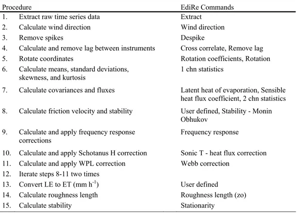
The sensible and latent heat fluxes were calculated using an averaging period of 15-min. Each adjustment step/procedure, mentioned above, was performed separately and then all steps were combined with the frequency response, WPL, and HFC adjustments being applied iteratively due to their interdependence. The sequence of adjustments is shown in table 1.
Table 1. Post-processing procedure using the software package EdiRe®.
Procedure EdiRe Commands
1. Extract raw time series data Extract
2. Calculate wind direction Wind direction
3. Remove spikes Despike
4. Calculate and remove lag between instruments Cross correlate, Remove lag
5. Rotate coordinates Rotation coefficients, Rotation
6. Calculate means, standard deviations,
skewness, and kurtosis 1 chn statistics
7. Calculate covariances and fluxes Latent heat of evaporation, Sensible heat flux coefficient, 2 chn statistics 8. Calculate friction velocity and stability User defined, Stability - Monin
Obhukov 9. Calculate and apply frequency response
corrections
Frequency response
10. Calculate and apply Schotanus H correction Sonic T - heat flux correction
11. Calculate and apply WPL correction Webb correction
12. Iterate steps 8-11 two times
13. Convert LE to ET (mm h-1) User defined
14. Calculate roughness length Roughness length (zo)
15. Calculate stability Stationarity
The canopy heights for both the Northeast (NE) and Southeast (SE) fields were measured five times during the study on the following DOYs: 171, 182, 200, 210, and 220. The canopy height shortly after emergence (DOY153) was assumed to be 0.01 m. The canopy height (hc, m) and DOY was plotted and a curve was fitted using SigmaPlot
11(Systat Software Inc., San Jose, CA) to determine the canopy height as a function of the DOY. The zero-plane displacement height was assumed to be 65% of the canopy height (Campbell and Norman 1998). The following functions correspond to the canopy height (m) for the NE and SE fields, respectively:
(6)
Wind direction, heat flux source area, stationarity, and integral turbulence tests were applied to filter out any data that did not meet minimum quality control standards. Only fluxes for wind directions between 142° and 322° from North were included in this study because the predominant wind direction and larger fetch were obtained from the south-southwest sector of the field. These parameters were set for two reasons: to achieve optimum inter-comparison between the EC systems and lysimeter ETc values and to
exclude flow that may be distorted by the instrumentation.
The approximate analytical heat flux source area (i.e. footprint) model proposed by Hsieh (2000) was used to calculate the 70% effective fetch. The distance upwind from the measurement location representing a fraction, f, of the contributing source area,
Xf (m), was calculated as:
(8)
with
(9)
where zo is the roughness length (m), zm is the wind measurement height (m), k is von
Karman’s constant (0.41), and D and P are the coefficients found by regression of Calder’s analytical solution (1952) to the results of Thompson’s Lagrangian model (1987) for unstable (D=0.28, P=0.59), near-neutral (D=0.97, P=1), and stable
stratification (D=2.44, P=1.33). To ensure reasonable horizontal homogeneity (i.e., that heat fluxes belonged within the cotton field), fluxes with effective fetch greater than the boundaries of the field were excluded. Measurements of heat fluxes via the eddy covariance method are based on simplified forms of the Navier-Stokes equations for certain atmospheric conditions (Stull, 1988). These conditions are not always met and therefore must be tested. Tests for stationarity and integral turbulence were performed following methods outlined in Foken and Wichura (1996) and Thomas and Foken (2002). For the stationarity test, covariances between the vertical wind speed (w) and the
horizontal wind speed (u), the air temperature (T), and the water vapor (q) scalars for the averaging period (i.e., 15-min) were compared to covariances of consecutive 5-min intervals within the same period. The periods where deviations, Δst, were greater than
30% were considered unstationary and excluded from the study:
where, x is u for momentum flux and the scalar of interest (T or q) for scalar fluxes and “5” and “o” are subscripts for the 5-min and averaging period covariances, respectively. Integral turbulence tests are used to determine if the turbulence is well developed. With weak turbulence the measuring methods based on surface layer similarities may not be valid (Foken et al., 2004). The integral turbulence test was done by comparing similarity functions for vertical wind speed (φw) and temperature (φT) with modeled functions
developed by Thomas and Foken (2002) as follows:
(11)
(12) where, σw and σT are the standard deviations of w and T, respectively, and T* is the
dynamic temperature (°C). Any periods with deviations between measured and modeled similarity functions, ΔITT, greater than 30% were excluded using the following:
(13)
Energy balance residual and statistical analysis
The effectiveness of each method of adjustment was determined by evaluating the energy balance residual and comparisons between the lysimeters ETc-measured values and
EC-measured/adjusted ETc values. The energy balance residual (ε) is defined as:
(14) Energy balance closure is achieved when the residual is equal to zero. Also, the energy balance ratio (EBR) is defined as:
(15)
The statistical analysis was performed following Willmott (1982). The mean bias error (MBE, Eq. 16), RMSE (Eq. 17), index of agreement (d, Eq. 18), and linear regression analysis based on the least squares method for comparison of fitted equation slope and intercept were used for the comparison of ETc values and evaluation of the entire
(16) where, N is the number of pairs compared, X(M)i is the measured EC-based ETc value,
and X(O)i the observed lysimeter-based ETc expressed in mm h-1 and percent (% of the
observed) .
The RSME and d were computed as follows:
(17)
(18)
RESULTS AND DISCUSSION
The individual and combined adjustment schemes were first evaluated by comparing EC and lysimeters measured ETc values. The level of energy balance closure was then
evaluated for each adjustment scheme. The MBE of EC-based hourly ETc before any
adjustments were applied was -0.13 mm h-1 (-26.9%) for site EC1 and -0.11 mm h-1 (-24.9%) for site EC2. A negative MBE means that the EC system underestimated ETc. Adjustment scheme evaluation
The WPL adjustment increased the MBE of EC-based hourly ETc to -0.13 mm h-1
(-29.5%) for site EC1 and -0.11 mm h-1 (-28.8%) for site EC2. Nighttime ET was 7-10% of the whole day ETc (Tolk et al. 2006a, b) and therefore even small variations will
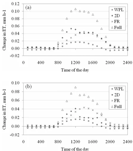
appear large in terms of percent. As shown in Figure 1, the hourly ETc values obtained
after applying the WPL adjustment resulted in a nighttime adjustment that was negative and in a daytime adjustment that was positive. Liebethal and Foken (2003) showed that the diurnal pattern of WPL adjustments correlated well with the diurnal pattern of vertical wind velocity. Although, the WPL adjustment increased the MBE while the RMSE decreased by a small amount. Considering only daytime EC-based ETc values (~14 h),
the MBE after WPL adjustments was -0.19 mm h-1 (-29.8%) with RMSE of 0.25 mm h-1 (27.4%) for EC1, and -0.16 mm h-1 (-27.2%) with RMSE of 0.19 mm h-1 (23.1%) for EC2. As shown in Liebethal and Foken (2003), the WPL adjustment had a much larger impact on CO2 flux. However, in our study the impact of WPL adjustments on ETc was
significant.
The 2D rotation adjustment improved hourly ETc for both EC sites having a more
significant impact on site EC1. For site EC1 the 2D adjustment reduced the MBE to -0.11 mm h-1 (-21.2%) and RMSE to 0.18 mm h-1 (20.7%). As shown in Figure 1, the 2D
adjustment was larger earlier in the day (morning hours). Although, the diurnal pattern was similar for both sites the magnitude was larger for EC1. This inconsistency could be due to a slightly different topography/micro-topography between the two sites or because one of the sensors was not leveled identical to the other.
Figure 1. Hourly average change of EC-based ETc due to Webb density (WPL), double
coordinate rotation (2D), frequency response (FR), and iteration of all adjustments (Full) from (a) northeast (NE) and (b) southeast (SE) fields for entire data set
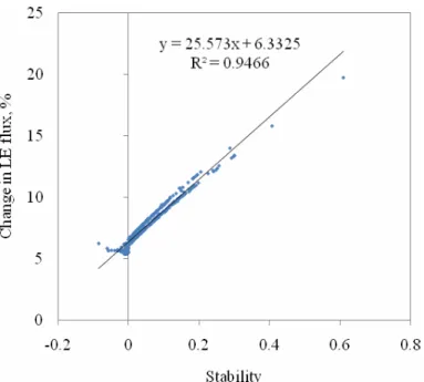
The frequency response (FR) adjustment had the most significant impact on EC-based hourly ET. The MBE and RMSE each decreased to -0.11 mm h-1 (-21.9%) and 0.18 mm h-1 (21.1%) for EC 1 and -0.09 mm h-1 (-19.5%) and 0.13 mm h-1 (17.3%) for EC2, respectively. The FR adjustment is mostly dependent on the sensor setup and method used to detrend the data, which was identical for both sites, and therefore similar results could be expected when using the same sensor setup and methods at different sites. As shown in Figure 2, there was a strong correlation between change in flux due to
frequency response adjustment and the atmospheric stability. As the atmosphere became more stable the impact of the adjustment increased. It should be noted that for unstable conditions (i.e. stability less than zero) the change remained the same, just above 5%.
Figure 2. Change in latent heat flux (%) due to frequency response adjustment versus atmospheric stability
The full adjustment of ET included 2D, FR, HFC, and WPL with the last three corrections being iterated two times due to their interdependence. Though the HFC doesn’t directly affect the ETc, it does affect H which was used in the calculation of the
WPL adjustment. The full adjustment of ET resulted in a MBE of -0.09 mm h-1 (-19.0%) for EC1 and -0.08 mm h-1 (-21.0%) for EC2. Table 2 details the ETc errors in mm h-1,
percent, and the corresponding correlation parameters for both EC systems and for ETc
including/excluding different adjustment schemes. Similar analyses of ET errors were performed for 15-min average ETc derived from daytime (~14 h) and are shown in Table
3. Also, the daily progress of energy fluxes and ETc rates during DOY 239 are illustrated
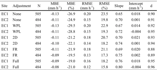
Table 2. Comparison of EC-based ETc with lysimetric ETc using the entire day (24 h)
15-min averaged data and different adjustment schemes
Site Adjustment N (mm hMBE -1) MBE (%) (mm hRMSE -1) RMSE (%) Slope Intercept (mm h-1) d
EC1 None 505 -0.13 -26.9 0.20 23.5 0.65 0.018 0.90 EC2 None 484 -0.11 -24.9 0.15 19.8 0.70 0.001 0.91 EC1 WPL 505 -0.13 -29.5 0.20 22.9 0.67 0.014 0.92 EC2 WPL 484 -0.11 -28.8 0.15 19.3 0.72 -0.004 0.95 EC1 2D 505 -0.11 -21.2 0.18 20.7 0.70 0.021 0.93 EC2 2D 484 -0.10 -22.1 0.14 18.2 0.74 0.001 0.94 EC1 FR 505 -0.11 -21.9 0.18 21.1 0.69 0.020 0.88 EC2 FR 484 -0.09 -19.5 0.13 17.3 0.75 0.002 0.89 EC1 Full 505 -0.09 -19.0 0.16 18.2 0.76 0.018 0.95 EC2 Full 484 -0.08 -21.0 0.12 15.8 0.80 -0.004 0.96
where, ETc is crop evapotranspiration, N is the sample size, MBE is the mean bias error, RMSE is
the root mean squared error, d is the index of agreement, EC1 is eddy covariance system 1, EC2 is eddy covariance system 2, WPL is Webb density correction, 2D is double coordinate rotation, FR is frequency response, and Full is the combination and iteration of all adjustments.
Table 3. Comparison of EC-based ETc with lysimetric ETc using daytime (~14 h) 15-min
averaged data and different adjustment schemes
Site Adjustment N (mm hMBE -1) MBE (%) (mm hRMSE -1) RMSE (%) Slope Intercept (mm h-1) d
EC1 None 320 -0.20 -30.8 0.25 28.2 0.61 0.050 0.82 EC2 None 290 -0.17 -28.2 0.20 24.0 0.71 -0.001 0.84 EC1 WPL 320 -0.19 -29.8 0.25 27.4 0.62 0.050 0.85 EC2 WPL 290 -0.16 -27.2 0.19 23.1 0.72 -0.003 0.89 EC1 2D 320 -0.16 -24.8 0.22 24.7 0.65 0.060 0.85 EC2 2D 290 -0.15 -24.4 0.18 22.0 0.73 0.002 0.88 EC1 FR 320 -0.17 -26.3 0.23 25.3 0.65 0.052 0.77 EC2 FR 290 -0.14 -23.1 0.17 20.9 0.75 0.000 0.79 EC1 Full 320 -0.13 -19.3 0.19 21.4 0.70 0.062 0.89 EC2 Full 290 -0.12 -18.9 0.15 18.5 0.80 0.000 0.92
where, ETc is crop evapotranspiration, N is the sample size, MBE is the mean bias error, RMSE is
the root mean squared error, d is the index of agreement, EC1 is eddy covariance system 1, EC2 is eddy covariance system 2, WPL is Webb density correction, 2D is double coordinate rotation, FR is frequency response, and Full is the combination and iteration of all adjustments.
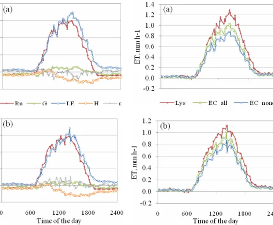
Figure 3. Diel net radiation (Rn), soil heat
flux (G), latent heat flux (LE), sensible heat flux (H), and residual (ε) (DOY 239) from (a) northeast (EC1) and (b) southeast (EC2)
fields
Figure 4. Diel lysimeter ETc (Lys), eddy
covariance with no adjustment (EC_none), and eddy covariance with iteration of all adjustments (EC_all) (DOY 239) from (a)
northeast (EC1) and (b) southeast (EC2) fields
Energy balance evaluation
Energy balance closure for non-adjusted fluxes was 89% and 83% for EC1 and EC2,
respectively. Each adjustment increased closure, with the 2D and FR adjustments having the most significant impact on improving the energy balance closure. The overall energy balance ratio for adjusted fluxes was 97% and 88% for EC1 and EC2, respectively. Table 4 shows the energy balance ratio, correlation parameters, and residual statistics in W m-2 for daytime (~14 h) fluxes. The daytime values of H were frequently negative as shown for DOY 239 in Figure 3. Irrigated land in the Texas High Plains is surrounded by very dry fallow lands and therefore the advection of dry heat can significantly increase ETc (Tolk et al., 2006b). However, the energy
balance closure did not reach 100% after adjustments were performed. Twine et al. (2000) discussed a method of closing the energy balance by preserving the Bowen ratio that could further improve the agreement between EC and lysimeter ETc values.
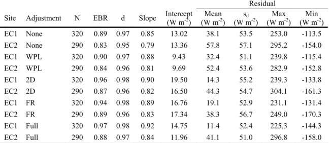
Table 4. Comparison of available energy (Rn-G) and turbulent heat flux energy (H+LE) using daytime (~14 h) 15-min averaged data and different adjustment schemes
Residual
Site Adjustment N EBR d Slope Intercept (W m-2) (W mMean -2) (W msd-2) (W mMax -2) (W mMin -2)
EC1 None 320 0.89 0.97 0.85 13.02 38.1 53.5 253.0 -113.5 EC2 None 290 0.83 0.95 0.79 13.36 57.8 57.1 295.2 -154.0 EC1 WPL 320 0.90 0.97 0.88 9.43 32.4 51.1 239.8 -115.4 EC2 WPL 290 0.84 0.96 0.81 9.69 52.4 53.6 282.9 -152.8 EC1 2D 320 0.96 0.98 0.90 19.50 14.3 55.2 239.3 -133.8 EC2 2D 290 0.87 0.96 0.82 16.50 44.3 54.7 304.1 -161.3 EC1 FR 320 0.94 0.98 0.89 16.76 19.1 52.9 231.1 -131.4 EC2 FR 290 0.89 0.96 0.83 17.34 38.3 56.7 249.0 -170.3 EC1 Full 320 0.97 0.98 0.92 14.75 11.4 52.4 225.3 -144.3 EC2 Full 290 0.88 0.97 0.84 11.96 41.1 51.0 296.8 -158.0
where, ETc is crop evapotranspiration, N is the sample size, MBE is the mean bias error, RMSE is the root
mean squared error, d is the index of agreement, EC1 is eddy covariance system 1, EC2 is eddy covariance system 2, WPL is Webb density correction, 2D is double coordinate rotation, FR is frequency response, and Full is the combination and iteration of all adjustments.
CONCLUSION
Accurate crop evapotranspiration measurements are important for irrigation management and model verification. Eddy covariance measurements of LE can be improved considerably when adjusted for vapor density, coordinate rotation, frequency response, and heat flux conversion. Double coordinate rotation and frequency response adjustments had the largest impact on properly adjusting EC-based ET. The coordinate rotation adjustments improved the MBE between EC-based hourly ET and lysimeter ET values by 5.7% and 2.8% for site EC1 and EC2, respectively. The frequency response adjustment improved MBE by 5.0% and 5.5% for site EC1 and EC2, respectively. The iteration of the entire combined adjustments improved the EC-based hourly ET by 3-8% and reduced the energy balance residual by 20-50%.
After adjustment EC still underestimated ET by 20%. It seems that further adjustments are needed beyond the procedures presented in this study. Large eddy flux contribution can only be measured if the averaging period is sufficiently long. This study was limited to a 15-min
averaging period and an optimum averaging period in which most of the flux can be measured without violating stationarity limits needs to be determined by testing longer averaging periods. Techniques to fill the gaps left by quality control procedures along with forcing energy balance closure could also be employed to further improve the EC-based ETc results. It is the
recommendation of the authors that the combined adjustment scheme described be consistently applied when using EC to properly measure ETc using EC systems.
REFERENCES
Burba, G, and Anderson, D (2007). Introduction to the Eddy Covariance Method: General Guidelines and Conventional Workflow. LI-COR Biosciences, http://www.licor.com , 141 pp (accessed 5 February 2010).
Campbell, GS, and Norman, JM (1998). An Introduction to Environmental Biophysics (2nd ed.). Springer, New York, 286 pp.
Clement, R (1999). EdiRe Data Software (Version 1.5.0.10) [Computer software]. Edinburgh, England: University of Edinburgh. Retrieved 1 March 2010. Available from
http://www.geos.ed.ac.uk/abs/research/micromet/EdiRe
Foken, T, and Wichura, B (1996). Tools for quality assessment of surface-based flux measurements. Agricultural and Forest Meteorology, 78:83-105.
Foken, T, Gockede, M, Mauder, M, Mahrt, L, Amiro, B, and Munger, W (2004). Post-field data quality control. In X Lee, W Massman, & B Law, Handbook of Micrometeorology: A Guide for Surface Flux Measurement and Analysis. Kluwer, Dordrecht, 181-208.
Howell, T, Schneider, A, Dusek, D, Marek, T, and Steiner, J (1995). Calibration and scale performance of Bushland weighing lysimeters. Trans ASAE, 38:1019-1024.
Hsieh, C, Katul, G, Chi, T (2000). An approximate analytical model for footprint estimation of scalar fluxes in thermally stratified atmospheric flows. Adv. Water Resour. 23:765-772. Kaimal, J, Finnigan, J (1994). Atmospheric Boundary Layer Flows: Their Structure and Measurement. Oxford University Press, New York, 289 pp.
Lee, X, Massman, W, and Law, B (2004). Handbook of Micrometeorology: A Guide for Surface Flux Measurement and Analysis. Kluwer, Dordrecht, 250 pp.
Liebethal, C, and Foken, T (2003). On the significance of the Webb correction to fluxes. Bound.-Layer Meteor. 109:99-106.
Mahrt, L (1998). Flux sampling error for aircrafts and towers. J Atmos. Oceanic Technol. 15:416-429.
Marek, T, Schneider, A, Howell, T, and Ebeling, L (1988). Design and installation of large weighing monolithic lysimeters. Trans ASAE, 31:477-484.
McMillen, R (1988). An eddy correlation technique with extended applicability to non-simple terrain. Bound.-Layer Meteor. 43:231-245.
Moore, C (1986). Frequency resopnse corrections for eddy correlation systems. Bound.-Layer Meteor., 37:17-35.
New, LL (2005). Agri-Partner irrigation result demonstrations 2005. Texas Cooperative Extension Servic, Texas A&M University. Available online at:
http://amarillo.tamu.edu/programs/agripartners/irrigation2005.htm
Rose, C and Sharma, M (1984). Summary and recommendations of the workshop on evapotranspiration of plant communities. Agric. Wat. Manag. 8:325-342.
Schotanus, P, Nieuwstadt, F, & De Bruin, H (1983). temperature measurement with a sonic anemometer and its applications to heat and moisture fluxes. Boundary-Layer Meteorology, 26:81-93.
Stull, RB (1988). An Introduction to Boundary Layer Meteorology. Kluwer, Dordrecht 666 pp. Thomas, C, & Foken, T (2002). Re-evaluation of integral turbulence characteristics and their parameterizations. Proceedings of the 15th Symposium on Boundary Layers and Turbulence (pp. 129-132). Wageningen, The Netherlands: Am. Meteorol. Soc.
Tolk, J, Howell, T, Evett, S (2006a). Nighttime evapotranspiration from alfalfa and cotton in a semiarid climate. Agron. J. 98:730-736.
Tolk, J, Evett, S, Howell, T (2006b). Advection influences on evapotranspiration of alfalfa in a semiarid climate. Agron. J. 98:1646-1654.
Twine, TE, Kustas, WP, Norman, JM, Cook, DR, Houser, PR, Meyers TP, Prueger, JH, Starks, PJ, Wesley, ML (2000). Correcting eddy covariance flux underestimates over a grassland. Agric. For. Meteorol. 103(3):229-317.
Webb, E, Pearman, G, & Leuning, R (1980). Correction of flux measurements for density effects due to heat and water vapour transfer. Quart. J. Roy. Meteorol. Soc., 106:85-100.
Willmott, CJ (1982). Some comments on the evaluation of model performance. Am. Meteor. Soc., 63:1309-1313.