Uppsala University
Independent Project in Electrical Engineering
Navigation robot
Authors:
Artur Absalyamov
Jimmy Gladh
Supervisor:
Ping Wu
Subject Reviewer:
Mats Ekberg
Examiner:
Mikael Bergkvist
August 7, 2020
ELEKTRO-E 20008
Abstract
Journeying into the information era the need for new technologies used for sending vast amounts of data efficiently has risen, as has the possibilities and need for different types of AI-controlled robots. In this project a RC-car was modified and equipped with a Raspberry PI and laser radar to let it automatically navigate around a room using UWB transmitters and receivers. A framework for robotic applications called ROS, Robot Operating System, was used with a large number of open source packages to fill different functions. Custom scripts was created to tie everything together, allowing all different components in the system to work in unison.
Popul¨
arvetenskaplig sammanfattning
S˚a kallad Ultra-wideband-teknologi, UWB, ¨ar en typ av radios¨andningar som kommit att anv¨andas mer och mer dem senaste ˚aren. Behovet av fler s¨att att skicka information p˚a har vuxit med v˚ar f¨ard in i interneteran. Det ¨ar d¨ar UWB kommer in, det ¨ar n¨amligen m¨ojligt f¨or en dator att skicka stora m¨angder information med teknologin j¨amf¨ort med traditionell radioteknik.
Som namnet antyder bygger det hela p˚a att man anv¨ander ett mycket vidare spann av frekvenser f¨or att skicka signalen. En radiokanal, s¨ag Rix FM, skickar sina s¨andningar p˚a en specifik frekvens, med en felmarginal p˚a s¨ag en tiondels Hertz n¨ar du justerar din radioapparat. UWB anv¨ander frekvenser ¨over ett spann p˚a 500 MHz. F¨or att inte st¨ora ut befintlig radiotrafik anv¨ander man en mycket svagare signal. En radiomast har en r¨ackvidd p˚a n˚agon mil beroende p˚a terr¨angen och din UWB s¨andare kanske p˚a sin h¨ojd kan s¨anda ut information p˚alitligt i ditt hus och inte l¨angre, det vill s¨aga ungef¨ar 10 meter.
I det h¨ar projektet har denna teknologi anv¨ands f¨or att best¨amma positionen f¨or en radiostyrd bil. Fem UWB-moduler har anv¨ants f¨or ¨andam˚alet, fyra som master i h¨ornen p˚a ett rum och en p˚a bilen. Teknologin ¨ar perfekt f¨or den h¨ar typen av applikationer d˚a den ¨ar snabbare ¨an vanliga radiosignaler. Positionen p˚a ett objekt i r¨orelse kan best¨ammas blixtsnabbt med centimeterprecision.
F¨or att nu styra bilen beh¨ovs mer ¨an master och mottagare, i projektet anv¨ander vi en Raspberry PI, en liten dator, f¨or att k¨ora alla program som beh¨ovs. Datorn k¨ors med operativsystemet Ubiquity, vilket ¨ar designat som ett l¨attviktssystem f¨or robotap-plikationer, specifikt f¨or ROS, Robot Operating System. Detta ¨ar ett ramverk som g¨or kommunikation mellan olika delar i ett system l¨attare. S¨ag att vi vill styra en robotarm till ett objekt. D˚a beh¨over vi s¨ag tre sensorer, tv˚a som k¨anner av var armens servomo-torer befinner sig och en som ser hur l˚angt borta objektet ¨ar. Alla dessa sensorer m˚aste kommunicera med en dator som i sin tur skickar signaler till motorerna beroende p˚a vad sensorerna rapporterar. Det ¨ar kommunikationen mellan alla dessa delar som ROS g¨or enklare genom att standardisera dess struktur. Vi kan ha tre olika utvecklare som skriver program till var del av robotarmen i var sitt programmeringsspr˚ak och det ska inte spela n˚agon roll, f¨or kommunikationen ¨ar standardiserad till en form.
ROS ¨ar ett open source-projekt med massvis med olika typer av paket man fritt kan ladda ner ifr˚an sidor som githhub. N˚agra s˚adana paket har anv¨ands i v˚art projekt. Vi anv¨ander till exempel en lidar f¨or att detektera hinder runtomkring bilen. Till denna lidar f¨oljer det med mjukvara anpassat f¨or ROS som vi fritt kan modifiera och anv¨anda. Informationen kan vi sedan anv¨anda i andra paket f¨or att l˚ata v˚ar bil navigera runt hinder kring sin rutt.
F¨or att ge bilen instruktioner programmerades en webserver med grafisk representation av bilen och masternas positioner. Man kunde i en webbrowser klicka p˚a ett rutn¨at f¨or att ge bilen en destination, och man kunde med en panel ge bilen direkta instruktioner f¨or att k¨ora den helt manuellt.
Contents
1 Introduction 1
1.1 Background and goals . . . 1
1.2 Method . . . 1
2 Theory 2 2.1 Sensor measurements . . . 2
2.1.1 Inertial Measurement Unit . . . 2
2.1.2 Distance measurement . . . 2
2.1.3 Position . . . 2
2.2 RC car motor control . . . 2
2.3 PID regulator . . . 3
2.4 UWB - Ultra-wideband . . . 3
2.5 Extended Kalman Filters . . . 4
2.6 Path-planning and obstacle avoidance . . . 5
2.6.1 A* algorithm based path planner . . . 5
2.6.2 Dijkstra’s algorithm based planner . . . 5
2.7 A positioning system . . . 6 2.8 Signal processing . . . 7 2.8.1 Frequency elimination . . . 7 2.8.2 Noise elimination . . . 7 3 Implementation 8 3.1 ROS . . . 8
3.1.1 User communication with ROS . . . 8
3.2 Hardware . . . 9
3.2.1 The RC-car . . . 9
3.2.2 Computers and inter-connectivity . . . 10
3.2.3 Adafruit 9DOF IMU . . . 11
3.2.4 MDEK1001 Development kit . . . 11
3.2.5 Slamtech RPLIDAR 360◦ Laser Range Finder . . . 12
3.2.6 The whole systems hardware . . . 13
3.3 The whole system represented with flowcharts . . . 14
3.4 Web-server . . . 15
3.4.1 React . . . 15
3.5 Software . . . 15
3.5.1 Frame handling . . . 15
3.5.2 Open source ROS packages utilized . . . 16
3.5.3 Custom ROS package . . . 16
3.5.4 Navigation stack . . . 18
3.5.5 Velocity commands interpretation . . . 18
3.5.6 ROS-tools for data collection . . . 19
4 Results 21 4.1 Server with React and Worldview . . . 21
4.2 The car in motion . . . 21
4.3 Performance of the IMU unit and Adafruit package . . . 22
4.5 Performance of the complementary filter package . . . 24
4.6 Performance of the UWB modules and robot localization package . . . . 25
4.7 Perforamnce of the PID package . . . 27
4.8 Performance of the rplidar package . . . 27
4.9 Performance of the navigation stack packages . . . 27
5 Discussion 28 5.1 Limitations of required knowledge . . . 28
5.2 ROS . . . 28
5.3 Some comments on Node.js and the server . . . 28
5.4 Acceleration drift . . . 29
5.5 IMU . . . 29
5.6 UWB modules and EKF . . . 29
5.7 The navigation stack . . . 30
5.8 Miscellaneous . . . 30
5.8.1 Under voltage problem . . . 30
5.8.2 Stuttering GPIO PWM output . . . 30
5.8.3 The movable base . . . 31
5.8.4 Pro tip . . . 31
5.8.5 Rviz . . . 31
6 Conclusions 31
7 References 32
A Topics and Messages they contain B Graph of ROS nodes and topics
Nomenclature
A∗ A-star
AP I Application Programming Interface BEC Battery Eliminator Circuit
EKF Extended Kalman Filter ESC Electronic Speed Control GP IO general-purpose-input-output GP S Global Positioning System I2C Inter-Integrated-Circuit
IM U Inertial Measurement unit Lidar Laser range finder
M EM S Microelectromechanical systems P ID Proportional-integral-derivative P W M Pulse Width Modulation RC Radio Controlled
ROS Robotic Operating System SSH Secure Shell
1
Introduction
1.1
Background and goals
The purpose of this project was to create a system for controlling a RC-car using UWB modules, creating a GPS-like system of communication. It was a continuation of a project that ended before completion. [1] The overall goals were to:
• Create a Ultra Width Band Controlled RC-car capable of navigating to a given position.
• Implement an Extended Kalman Filter for position estimation and prediction. • Creating a system for controlling the car with manual inputs.
• Implement a system to make the robot aware of obstacles with distance detection using a lidar.
• Use a local web server to graphically present data on the fly.
1.2
Method
The project was to be completed using a framework for robotics called ROS, Robot Operating System, which offers a widely used system capable of handling different pro-gramming languages, and offering many open source packages. Hence the project was focused around implementation and deployment of open source software and not devel-opment.
The system consisted of Decawave receivers and transmitters, a web server, a Raspberry PI and a Reely RC-car. The Raspberry PI ran the operating system Ubiquity, a light weight system based on Linux, designed for ROS. Sensors used was a IMU chip from Adafruit and a lidar system from Slamtech. The web server was created with Java script Node, with the packages React and Worldview.
In short, the IMU chip made it possible to calculate and track the pose of the car, inclination and position. It fused the data from an accelerometer, a gyroscope and a magnetometer that senses applied force, inclination and the direction of earths magnetic field respectively. The lidar is a 360◦laser radar that can detect and calculate the distance to obstacles.
All these parts were tied together by ROS, using custom made scripts and drivers supplied for the sensors by its respective manufacturer. It made it possible to manually move the car with direct user input, track its position with the UWB network, and create scripts that let the car maneuver on its own.
2
Theory
2.1
Sensor measurements
For a robot to be able to act in the world with desired precision and outcome, some sensory inputs are required.
2.1.1 Inertial Measurement Unit
An IMU is an electronic device built to measure the data necessary to calculate a heading. It contains a gyro, an accelerometer and a magnetometer. The output from these readings is acceleration, angular velocity and compass readings. With this information, a computer or IC can be used to fuse all readings into a heading. [2]
2.1.2 Distance measurement
From a robotic perspective distance measurement can be accomplished directly with two methods; ultrasonic distance measurement and laser distance measurement. To get the distance to objects around a robot, a radar or a lidar may be used, where the radar utilises the ultrasonic distance measurement and the lidar the laser distance measurement. Both types usually tracks the angle to the detected objects. Distance can also be measured indirectly, with the most prominent method being calculation of distance using position tracking and known obstacle positions.
Ultrasonic distance measurement works by the usage of sound waves with typical fre-quencies of 40kHz. By transmitting sound waves out from a transducer and receiving the bounced back wave with a receiver, the distance to an object can be calculated by the flight time of the sound wave.
Laser distance measurement works by the usage of directed light. In essence it works by the same principles as ultrasonic measurements, but generally demands more of the equipment used due to the nature of light.
2.1.3 Position
A prominent position tracking method is triangulation, and it can be achieved by mea-suring the time of flight of signals. As the name implies at least three static meamea-suring points are needed to pinpoint the position of the tracked object. There are many ways to do this, but using electromagnetic signals gives the most robust measuring option. An object position may also be calculated from velocity and known original position. Considering real world application this method is likely to contain errors, but it can be fused with triangulation measurements with different types of state filters, one prominent being the Kalman filter.
2.2
RC car motor control
A RC car may contain several types of motors, a servo motor and a DC motor are the two most prominent components. A servo motor can be described as a mechanical pointer, where the motor can rotate 180°. The position is determined by a 50Hz PWM signals bandwidth, seen in figure 1.
Figure 1: The position of a servo motor based on PWM signal bandwidth.
A DC motor on the other hand should be controlled by a motor driver feeding the motor a PWM power signal. This ensures direct control of the torque by a variable duty cycle. One controller to be noted is the ESC controller. This controller takes the same signal input as the servo motor, and if available on the model, allows a motor to run in reverse. If reversing is allowed, the throttle follows the same principle shown in figure 1, no throttle at 1.5ms bandwidth, full throttle in reverse at 1ms bandwidth and full throttle forward at 2ms bandwidth. If reversing is not available the throttle increases with the bandwidth from 1ms to 2ms. The ESC type controller is used in RC cars to ensure simplicity. [3]
2.3
PID regulator
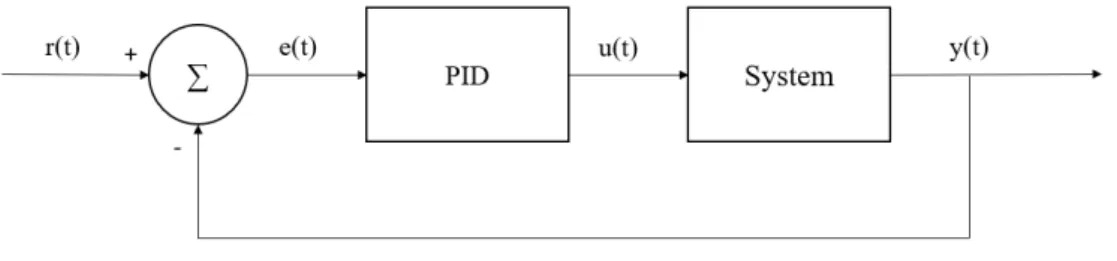
In control and system theory the PID regulator is a feedback regulator that adjusts the error signal to a system, as seen in figure 2.
Figure 2: PID regulated system flowchart.
The PID regulator acts on the error signal, producing three parts of the input signal u(t) to the system. The proportional part, where the error signal is multiplied by a constant KP. The integral part, where the error signal is integrated and then multiplied by a
constant KI. The derivative part, where the error signal is derived and then multiplied
by a constant KD. Which can be expressed with the following equation;
u(t) = Kpe(t) + KI Z t 0 e(t)dt + KD d dte(t) (1)
2.4
UWB - Ultra-wideband
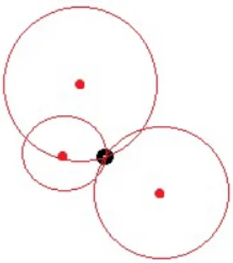
Ultra-wideband is a radio technology that uses a larger than normal portion of the spec-trum, allowing quicker communication at a much lower energy. This keeps it from inter-fering with other narrow band communication, which communicate by varying the power level or/and frequency of the signal. UWB communicates instead by sending pulses at set intervals. The technology allows for a very precise time of flight measurement, which can be used to triangulate the position of a object at very high speeds.
Figure 3: Triangulation of the black objects position with three anchors.
These pulses are easy to encode with information. The amplitude, polarity and phase can all be modulated for this purpose. With a known initial signal strength the time of flight can be determined by detecting the strength at the receiver.
To keep the signals from interfering with other radio signals, the signal strength is limited to −41.3 dBm/MHz at 3.1 GHz to 10.6 GHz by the FCC in USA, with similar regulations existing around the world. An UWB-signals bandwidth is defined as having a fractional bandwidth larger than 20% or sending information on a spread of over 500 MHz. [4]
2.5
Extended Kalman Filters
A Kalman Filter is a filter that converts state space data to, in the case of this project, a position. The input are acceleration, magnetic field strength and gyroscope data, and its associated measurement covariance, which is fused into an estimated pose. It can update estimations continuously as new data are received.
An ordinary Kalman Filter are used for linear systems, while an Extended Kalman Filter are used for nonlinear systems continually approximating the system as linear.
A state space system in this case is defined as,
xk+1= f (xk) + wk (2)
yk= h(xk) + vk (3)
where f and h are non linear equations that are approximated as linear around the present state of the system. w and v are static and measurement noise.
A car moving in 2 dimensions can be modelled as,
xk+1 = xk+ ˙xk∆t + 1 2x∆t¨ 2 (4) yk+1 = yk+ ˙yk∆t + 1 2y∆t¨ 2 (5) θk+1 = θk+ ˙θk∆t (6)
˙xk+1= ˙xk+ ¨x∆t (7)
˙
yk+1 = ˙yk+ ¨y∆t (8)
where x and y depicts the car position and θ its steering angle, at time indexes k. The complete state space system in matrix form becomes,
xk+1 yk+1 θk+1 ˙xk+1 ˙ yk+1 = 1 0 0 ∆t 0 0 1 0 0 ∆t 0 0 1 0 0 0 0 0 1 0 0 0 0 0 1 xk yk θk ˙xk ˙ yk + 1 2∆t 2 0 0 0 12∆t2 0 0 0 ∆t ∆t 0 0 0 ∆t 0 ¨ xk ¨ yk ˙ θk (9) xk yk θk = 1 0 0 0 0 0 1 0 0 0 0 0 1 0 0 xk yk θk ˙xk ˙ yk (10)
2.6
Path-planning and obstacle avoidance
For a robot to effectively navigate to a desired position a path planning algorithm should be used, preferably one that also allows the robot to avoid collisions on the way. Two different path planning algorithms are to be noted; Dijkstra’s and A*.
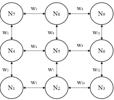
A* and Dijkstra’s algorithms use a graph network to compute the path to a desired destination. [5] A suitable graph network forming a map can be seen in figure 4, with nodes denoted N and edges containing a weight value denoted w. The graph network is a grid based map. Path finding algorithms are based on weight values between nodes. In a map style graph the weight values may represent distance or a stress factor for how suitable the path between two nodes is.
2.6.1 A* algorithm based path planner
The A* algorithm is path finding algorithm. The path is computed based on the actual distance to the goal and edge weights in a graph network. The algorithm computes the shortest path node to node, using the sum of edge weights and the remaining actual distance to the goal, meaning the produced path will be the most direct path, but not necessarily the shortest.
2.6.2 Dijkstra’s algorithm based planner
Dijkstra’s algorithm is based on finding the shortest path. The algorithm works by iter-ating over a graph network and saving paths summing the edge weights to a destination, similarly to the A* algorithm. However, the Dijkstra’s algorithm computes all the possi-ble paths to the goal without using the actual distance to the goal. The paths are saved in a priority queue, where the path with the lowest sum of the edge weights to the goal will be the output of the algorithm, and optimally will be the shortest path [5].
Figure 4: Representation of a graph network for a robotic application.
The A* and Dijkstra’s algorithms can plan a path around known obstacles, but a robot will still have to efficiently navigate around unknown obstacles. That can be achieved by continuously updating a graph map with obstacle data and computing new paths, thus creating simple obstacle avoidance.
2.7
A positioning system
UWB-signals are very good for precise measurements of a signals time of flight. Consid-ering a movable tag and four static anchors, which send pulses between each other, a high precision position of the tag can be triangulated by the time of flight of the signals.
2.8
Signal processing
2.8.1 Frequency elimination
To utilize sensors efficiently the signals received need to, at times, be filtered and pro-cessed. There are two digital filters that can be used to improve any signal: the low-pass filter and the high-pass filter. The low-pass filter filters out frequencies above a certain cut-off frequency and the high-pass filter filters out frequencies below a certain cut-off frequency. The filters are used to remove unwanted frequencies appearing in the sensor signal stream.
2.8.2 Noise elimination
A signal can also accumulate noise throughout the signal stream. In that case other filters need to be considered. The Wiener filters are to be noted. Theses filters are optimal in a mean-square error sense. [6] The filter produces an estimation of a signal based on a cost or error function which minimizes the mean square difference between the signal and the desired output. This filter is suitable for white noise sequence cancellation.
3
Implementation
3.1
ROS
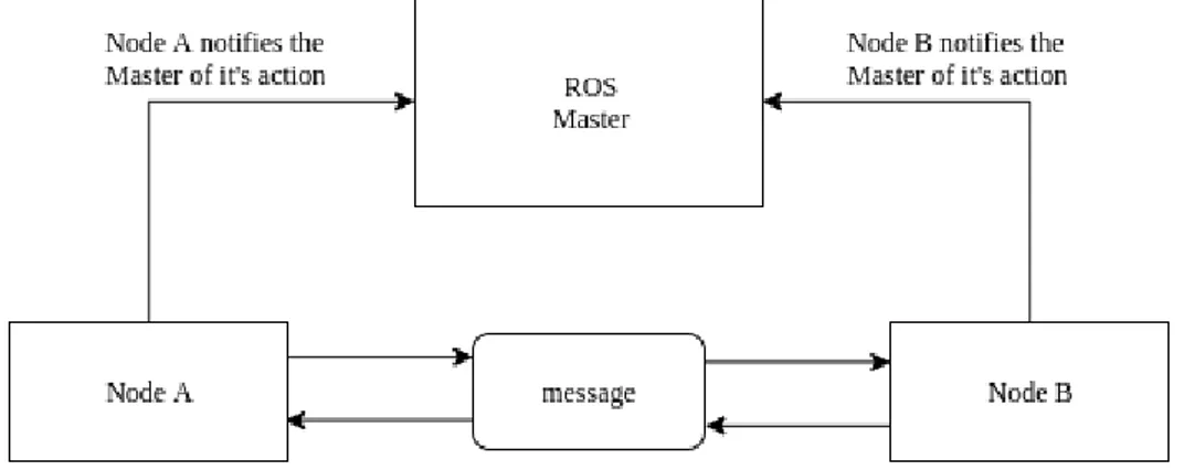
ROS is an open source system built to run on Linux based systems. ROS is a meta-operating system meaning that it utilizes software in packages to function [7]. The main reason ROS was used is because of its run-time communication system, where the commu-nication contained within messages can be efficiently and simply passed between different processing nodes, see Fig 6. The processes running on ROS are contained in nodes, and information passed between the nodes is contained in ROS custom message formats. The messages contain standard programming data types formatted to represent relevant in-formation. The nodes act as publishers, publishing messages, or subscribers, subscribing to messages, or acting as both at the same time. The ROS Master is a main process of the framework that tracks the publishers and subscribers enabling individual nodes to locate one another.
Figure 6: A diagram over the ROS communication.
A ROS framework contains two more used features running alongside the Master, a parameter server and a service server. The parameter server keeps track and allows dynamic updating of parameters specified in code lines. The service server allows nodes to communicate with services, a ROS custom request and deliver system, containing the same information as a standard message.
ROS works through a folder workspace where the software is contained in packages, which can contain any number of nodes working in parallel. Main ROS workspace works in the same fashion. Upon installation a workspace is used to run core ROS packages on the computer.
3.1.1 User communication with ROS
After initializing the desired ROS nodes there are several ways for a user to interact with running nodes. As ROS is built to run on a Linux based system, the user communica-tion happens through the terminal, where terminal commands can be issued to directly interact with the nodes, as the software allows it. Some useful terminal command-line tools are:
• rosnode
• rostopic
Used for information collection about running nodes, while also enabling the user to publish and subscribe to topics through the terminal.
• rosparam
Used for getting and setting parameters when nodes are running.
3.2
Hardware
3.2.1 The RC-car
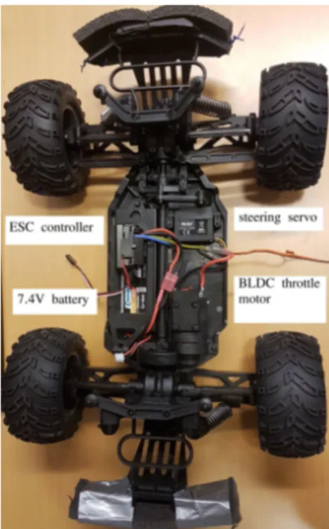
The RC-car provided for the project is a Reely Cyclone RC car with the decorative top and receiver removed, which can be seen in figure 7. The car was used as a movable base.
Figure 7: A picture of the RC car provided.
The car uses Ackermann steering to maneuver, where the inner wheel has a higher turning angle than the outer wheel as the wheels travels different distances while taking a turn [8]. The car is built with four wheel differential drive. The car contained two motors: A servo for the steering and a DC motor for the throttle, and also one ESC controller. The ESC controller contained a BEC regulator outputting 6V and 2A to the steering servo. The controller allowed the DC motor to drive in reverse whilst allowing the input of same signal type, servo control signals, to both the motors. The controller was configurable by junction connections, the reverse mode could be turned on and off, the battery type could be set to Lipo or NiMH. The controller self calibrated when first turned on, setting the input signal att the time to be the neutral value [9]. The car contained a 7.4V li-ion battery which delivered power to the motors.
It was found out that the 7.4V li-ion battery was faulty and did not work. Another battery was used instead, a 11.1V Lipo battery.
Since the steering was handled by servo motor the steering angle as an input could be described by the following equation;
φ = arctan l
r (11)
Where the turning angle is denoted φ, turning radius r and length of the car by l.
3.2.2 Computers and inter-connectivity
ROS required a Linux based computer to be able to fit on a mobile base. A lightweight option for this was a Raspberry PI. The Raspberry PI was powerful enough to run ROS and contained a 40 pin GPIO header, making external connections possible without the use of an external controller. A Raspberry PI 3 B+ was used for the project, see figure 8. It had a light weight operating system installed on it called Ubiquity Robotics [10], which is built on Ubuntu, a Linux distribution, specifically for usage with ROS. The Raspberry PI was used to run most of the software in the project through ROS Kinetic Kame, which is a distribution of ROS designed for Ubuntu 16.04.
Figure 8: A picture of the Raspberry PI 3 B+.
The Raspberry PI was used through a terminal on a laptop connected through a SSH connection. The laptop was used to prepare ROS packages and collect data. The laptop had Ubuntu operating system which was running ROS Melodic Morenia, a ROS distri-bution for Ubuntu 18.04. During installation of diverse non ROS related packages the Raspberry PI was connected and used as a standalone computer with a computer screen connected. The Raspberry PI was powered by two 5V , 1A out batteries.
Connection through SSH was made possible by a router running a local network, where the Raspberry PI was connected to the local network with WIFI, ensuring a movable base. The laptop could be connected to the local network either with a cable or through WIFI.
3.2.3 Adafruit 9DOF IMU
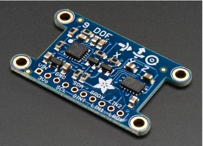
An Adafruit 9-DOF IMU Breakout - L3GD20H + LSM303 sensor board was used to measure angular velocity, magnetic field strength and acceleration data and was connected directly to the Raspberry PI through a I2C connection. The sensor board is a combination of two breakout boards provided by Adafruit, the board contains two sensors L3GD20H and LSM303, the board can be seen in figure 9. The L3GD20H is a 3-axis gyroscope sensor, and the LSM303 is a 3-axis accelerometer and a 3-axis magnetometer sensor.
Figure 9: The Adafruit 9DOF IMU. Source: www.adafruit.com
3.2.4 MDEK1001 Development kit
In the project a Decawave kit for UWB-applications was used. The kit consisted of 12 DWM1001 development boards. The modules were capable of transmitting and receiving signals, each board contained a microprocessor and a 3-axis motion detector, thus allowing position calculation to done on the board extracted through either a USB connection or a serial connection. The position was calculated with a 10cm standard deviation. Five modules were used to create a fully functioning system, one module was situated on the car, four were placed at a height in the corners of a room. This kit was used to track the position of the car. In figure 10 this can be seen in action through Devawaves android application, which was used to configure the tag and anchors. The module on the car communicated with the Raspberry PI through an USB-cable.
Figure 10: The interface of the Android app.
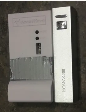
Figure 11: An UWB-module.
3.2.5 Slamtech RPLIDAR 360◦ Laser Range Finder
To make the car aware of its surroundings a Slamtech RPLidar A1 was used. It was mounted on the front of the car and connected to the Raspberry PI with an USB-cable. It detected obstacles around the car with a range of 12 meters and published the angle and distance in respect to the detector.
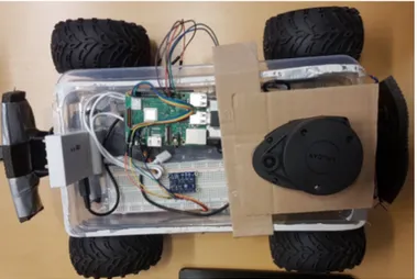
3.2.6 The whole systems hardware
The entire layout of the hardware, a plastic tray with the components haphazardly placed in or taped to it. A custom made cardboard mount was created for the lidar. A proper mounting made in Solidworks was designed but was not 3d-printed in time. It had four slots for batteries and a Decawave 1001 unit, screw holes for the IMU and Raspberry PI and a mounting for the lidar.
3.3
The whole system represented with flowcharts
In figure 13 through figure 15 data flows concerning different paths of the whole system are depicted.
Figure 13: Data flow concerning the Kalman filter
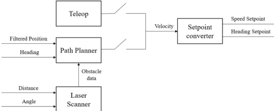
Figure 14: Data flow associated with path planning. The teleop block handles manual commands
Figure 15: Data stream for velocity control
3.4
Web-server
A web-server was created to graphically present all the positions of the car and anchors. A simple interface was also made to let the user send commands to the car. The server was coded with Node.js, React and an open source package called Worldview. It has a wide variety of functions allowing web developers to create interfaces and graphics for their web pages.
Figure 17: A mysterious cube, rendered with Worldview for unknown reasons. Bound by six sides, what evil does it contain? What madness would be release upon the world if ever breached? All hail the cube.
One server was already created at the start of the project. Parts of this program was used to create the server later used and was programmed in java script and HTML. It could present the position of the anchors and the tag, and had a interface for allowing direct control of the car. It also had a grid that the user could interact with to give the car instructions on where to drive. It used a Node.js ROS-package, ROSbridge, to handle this communication. The server was able to send messages back to the Raspberry PI running ROS and was abandoned for ROS based tools.
3.4.1 React
React is a widely use Java script node package designed to create apps and web pages. It was used to create the interface for the web-server. A package based on React called Worldview was used to graphically present tag and anchor positions.
3.5
Software
3.5.1 Frame handling
Frames in ROS are defined by the right hand rule, positive x-direction is forward, positive y-direction is left and positive z-direction is up. To handle transformations a ROS core tool called tf was used in the custom package nodes. The tf tool keeps track of frames, which for this project are only two. One frame for the world, denoted ”world”, and one frame for the movable base, denoted ”tag frame ekf”. One frame for the tag position and heading was used as a placeholder, denoted ”tag frame” The movable base frame is also contained in odometry messages, see appendix A for message definition.
3.5.2 Open source ROS packages utilized
The laptop used one package, the teleop twist keyboard package [11]. This package pub-lished velocity commands based on keyboard input on the ”/cmd vel” topic, this corre-sponds to ”Teleop” block in figure 14.
Names and descriptions of the open source ROS packages used on the Raspberry PI, see appendix A for topic message information. See appendix B for a graph over node to topic communication. See appendix C for a graph over parameter settings.
• adafruit imu
This package provided ROS drivers for the Adafruit 9-DOF IMU Breakout - L3GD20H + LSM303 sensor board [12], allowing data reading from the board. This package published on the ”/imu/data raw” and ”/imu/mag” topics. This corresponds to ”IMU” block in figure 13.
• imu complementary filter
This package provided orientation by fusing the accelerometer, magnetometer and gyroscope data obtained from the IMU [13]. This package subscribed to the data raw” and published the compiled IMU data and orientation on the ”/imu/-data” topic. This corresponds to ”Heading Calculator” block in figure 13.
• localizer dwm1001
This package provided position of the tag and the four latest anchors, obtained from serial communication with a DWM1001 development board [14]. This package published tag location on the ”/dwm1001/tag” topic and four anchor locations on four ”/dwm1001/anchor” topics. This corresponds to the ”UWB” block in figure 13.
• pid
This package provided a PID regulator [15] and error calculation. The package subscribed to ”/setpoint” and ”/state” topics and published on the ”/control effort” topic. This corresponds to the summation point and ”PID” block in figure 15. • robot localization
This package provided a ready to implement EKF, the package is able to fuse an arbitrary number of sensor messages to provide a state estimation [16]. This package subscribes to ”/imu/data ekf”, ”/odom” and ”/cmd vel” topics. Fusing the postion, acceleration and velocity commands, and published on ”/odometry filtered” topic. This corresponds to ”EKF” block in figure 13. This package could output velocity of the frame, obtained from position data difference and acceleration, the velocity did not however match an acceptable level of accuracy.
• rplidar
This package provided rplidar device drivers and laser scan transformations [17]. This package published on the ”/scan” topic. This corresponds to ”Laser Scanner” block in figure 14.
3.5.3 Custom ROS package
One package was created to control and compensate the open source packages. Containing several nodes written in Python, with names and descriptions below.
• turn angle and speed
This node subscribed to ”/odometry filtered” and ”/cmd vel” topics and published the robots desired speed on ”/setpoint” topic. The velocity of the robot on ”/state” topic and the the desired turn angle on ”/turn angle” topic. This node corresponds to the ”Setpoint converter” block in figure 14. The setpoint of the speed was given in the velocity commands linear x value, the turning angle setpoint was given by the velocity commands angular. As the velocity command is sent relative to the movable base frame, the summation point is in figure 16 is automatically built in the transformation. The ”abs” function outputted the absolute value of the velocity command, corresponding to the speed.
• Imu to ekf
This node subscribed to the ”/imu/data” and ”/cmd vel” topics and published IMU data based on the state of the robot to the ”/imu/data ekf” topic. When no velocity command is sent this node sets the acceleration to 0.
• tag odom broadcast
This node subscribes to ”dwm1001/tag” and ”/imu/data” topics and publishes on the ”/odom” topic. This node is meant to provide access to the heading calculated by the complementary filter package, where it can be transformed by an offset set as a parameter.
• car controller
This node was responsible for controlling two GPIO pins on the Raspberry PI and send PWM signals to the steering servo and ESC controller. The node subscribes to ”/control effort” and ”/turn angle” topics. The node utilized the pigpio python library for controlling GPIO pins on the Raspberry PI [18]. The pigpio library utilises a daemon server running on the Raspberry PI, through code commands GPIO channels could be controlled. Hardware PWM was used to send PWM signals to the motors, with the ”set servo pulsewidth” function, the function had an input of pulse width in µs. The PWM signal used followed the servo motor control logic where the input was (1000, 2000).
Two different libraries were tested previously to the pigpio library, RPI.GPIO and GPIO Zero. They but did not meet the requirements to control the motors. The classes ”Servo” and ”AngularServo” in the GPIO Zero library were tested. The ”Servo” class allowed a PWM servo control specific signal to be outputted through a GPIO pin. This class used input values of (−1, 1) to control the bandwidth of the PWM signal, from 1ms to 2ms. This was used to create a PWM to the ESC controller. The ”AngularServo” class works the same way ”Servo” class does, but takes input as an angle of (−90, 90). The GPIO Zero library also used the pigpio daemon server to control the GPIO channels [19].
The RPI.GPIO provided simple PWM output instance for the GPIO pins, ”GPIO.PWM”. Which took a duty cycle of (0, 100) as the input [20].
• acc integration
This node was responsible for integrating acceleration data to produce a velocity reading. The node subscribed to ”/imu/data raw” topic and published to ”/cur-rent twist” topic. The node utilized the python signal processing library SciPy.
From the library two classes were used,”signal.butter” and ”signal.weiner”. The ”signal.butter” was used to create a high pass filter to filter out stationary offset in the acceleration signal. The ”signal.weiner” was used to create a weiner filter and eliminate present noise, which was assumed to be white noise in the acceleration signal. Due to not acceptable velocity output this node was abandoned.
3.5.4 Navigation stack
The navigation stack is a compilation of different packages allowing for, path planning, localization and velocity command output [21]. The navigation stack allows a map to be used with the navigation, it was not used in this project. Several packages from the navigation stack were used, with names and descriptions below.
• move base
This package handled the velocity command generetaion and published these on ”/cmd vel” topic. This package computed velocity commands based on inputs of two different paths, one global path and one local path. This package is also responisble for launching other packages.
• costmap 2d
This package created an occupancy grid map, assigning cost values to two different maps. One map being a global map which could be loaded from a map file and a local map. This package subscribes to the ”/scan” topic.
• base local planner
This package produced a local path for the robot to follow using the local costmap. The package creates a kinematic trajectory by utilising the Trajectory Rollout and Window Approach algorithms.
• global planner
This package produced a global path for the robot to follow using the global costmap. This package utilized different path planning algorithms, including the A* and Dijkstra’s algorithms.
Mer kommer senare.
3.5.5 Velocity commands interpretation
The velocity commands sent by the ”teleop twist keyboard” and navigation stack pack-ages were set to be specified for a holonomic movable base, as Ackermann steering movable base was not supported by default.
The navigation stack packages updates velocity commands based on the heading of the ”tag frame ekf” frame, thus a steering response is created as seen in figure 18 after the velocity command in interpreted by the ”turn angle and speed” node.
The ”teleop twist keyboard” package did not update velocity commands based on heading of the movable base frame. Thus a steering response mimicking an RC car control is created as seen in figure 19.
Figure 18: Diagram of the steering systems response to velocity vector from the navi-gation stack. The coordinate system depicted is the cars system.
Figure 19: Diagram of the steering systems response to velocity vectors from the ”teleop twist keyboard” package.
3.5.6 ROS-tools for data collection
To compensate the web-server ROS basic data collection and visualization tools were used, these are packages which can be utilized to view ongoing processes and record them.
• Rviz
Rviz is a 3D visualisation tool suitable for visualizing scan results, observing frame transformations and publishing simple geometry messages, it was used to publish a goal position on ”/movebase base simple/goal”.
• rqt graph
This tool visualizes the message stream on ROS, node to node or node to topic information.
• rqt plot
• rqt bag
This tool used in combination with the rosbag command line tool allows visualiza-tion of recorded data with rosbag.
4
Results
4.1
Server with React and Worldview
The server was finished with some functionality. It had an interface that would have let the user give commands to the car, including panel with direct steering dials, and interactivity with the x-y-plane. Using Worldview, a React package for Node.js, all this information was presented graphically in the browser connected to the car. However, the server was not fully completed; only one way communication was possible where the server received subscribed topics but could not publish them. Due to time constraints data collection and visualisation was moved to ROS based tools.
4.2
The car in motion
Testing the node running the library GPIO Zero with the classes ”Servo” and ”Angu-larServo” showed that the motors could be controlled. The input limits were noted to be (−72°, 15°) for the ”AngularServo” class with an offset of −28.5°. The input limits for when the DC motor started moving the car were noted to be (−0.25, 0.15) for the ”Servo” class. It was observed that the car could reach high speeds, which were assumed unsafe for indoor environment.
When the node running the GPIO Zero library was used with the rest of the system it produced irregular motor performance when the input was zero. The DC motor did not work properly. Observing the PWM signals on an oscilloscope showed that the signal was stuttering, changing the duty cycle momentarily.
Testing the RPI.GPIO library instance, with the node running with the rest of the system, produced a PWM output following the same results as described above for the GPIO Zero library.
Testing the pigpio library with hardware PWM produced a PWM signal which did not stutter was observed with an oscilloscope, the motors did not have irregular performance. The pulse width limits for the steering motor were noted to be (1085, 1660) in µs, the steering angle was noted to be zero at 1400µs long pulse width. The limits for when the DC motor started moving the car were noted to be (1375, 1585) in µs.
The DC motor at times stopped working in reverse, it was discovered that the ESC controller required a signal change twice when changing directions to go backwards. A solution to this was implemented in the code lines, by changing the PWM output twice during a 30ms window. The hardware PWM did not shutdown at node shutdown, due to time constraints a solution was not discovered.
The ”teleop twist keyboard” set velocities as outputs using a speed component and an angular rotation component around the z-axis. The package was tested without the aid of speed regulation, instead the pulse width at which the DC motor started moving the car was used. When the car was in motion the steering response did follow the path seen in figure 19. No significant delay could be observed between the keyboard presses and the cars response. Manual control of the car was noted to be difficult due to high speed.
The lowest speeds forward and backwards were calculated by allowing the car to drive 3 meters, were the first meter counted for its acceleration, the time to drive the remaining
mean Forward (s) 2.64 1.51 1.44 1.58 1.51 1,96 2.11 2.17 2.04 1.98 1.80 Backward (s) 2.89 2.42 3.08 2.75 2.83 2,83 2.70 2.63 2.69 2.76 2.75
Table 1: Time measurements of the RC car speeds
two meters was noted, with mean value calculated, seen in the table 1. The lowest speed going forward was 1.11m/s and backward 0.73m/s. The turning radius was noted to be 0.9m.
4.3
Performance of the IMU unit and Adafruit package
The IMU unit and ”adafruit imu” package were tested by observing how acceleration and angular velocity changed during 60 seconds in stationary position with with normal orientation, it was working if the values did not diverge much from zero. To test the units acceleration during motion, the unit was rotated so each axis pointed towards the Earth and if the value of the acceleration was around 9.8m/s the unit was assumed to be working. The data was collected with rqt plot.
Figure 20: Stationary acceleration reading on x and y axis during 60 seconds
Figure 21: Stationary angular velocity reading on x, y and z axis during 60 seconds
The x-axis on the unit turned towards the earth showed a value around 9.8m/s, the y-axis turned towards the earth showed a value around 9.8m/s and the z-axis showed a
value of −9.8m/s during the stationary test. As the values seen in figures 20 and 21 do not diverge much from zero it was decided that the IMU unit and package were working properly.
The magnetometer was assumed to be working normally. Calibration equipment for magnetometer devices was not available. It was assumed, since the accelerometer was working the magnetometer was working as well, since both are contained within one chip, LSM303.
4.4
Acceleration integration
Recorded stationary acceleration data, as seen in figure 20, was analyzed with an FFT. A notable 0Hz spike was visible and decaying frequency components as the frequency increased. It was assumed that 0Hz spike represented an offset present and the rest of the frequency components were assumed to be white noise.
The acceleration could not be integrated to produce acceptable velocity values during stationary position, as seen in figures 22 to 24 where the velocity on both the x and y axis are diverging from zero. Different cut off frequencies on the high pass were tested, none produced acceptable velocity. The integration error was not reduced during movement and integration of acceleration to produce velocity was abandoned.
Figure 22: Stationary acceleration integration during 60 seconds using a high pass filter with a cutoff frequency off 1Hz.
Figure 23: Stationary acceleration integration during 60 seconds using a wiener filter
Figure 24: Stationary acceleration integration during 60 seconds using a high pass filter with a cutoff frequency off 1Hz and a wiener filter.
To aid the integration switching the power supplied to the Raspberry PI was tried, it was assumed it could aid the sensor measurements since the Rapsberry PI detected under voltage. The power supply was changed from one 5V , 1A out battery to three. Using three batteries showed that one battery turned off, two batteries could be used at the same time. This approach did not produce any difference for the integration.
One attempt to aid the integration was to analyze how the software in the package ”adafruit imu” outputted the acceleration data and rewrite parts of the code. It was discovered that the acceleration data was outputted by cumulative mean calculation. It was attempted to change the sample size, this did not produce any difference for the integration.
To compensate for the unsuccessful integration of the accelerometer data the possibility of using velocity calculation in the ”robot localization” package was investigated.
4.5
Performance of the complementary filter package
The package was tested in Rviz by visually observing two events and tuning the param-eters of the package until acceptable results were observed. The heading when the filter
started and the heading when the IMU unit was rotated 90° to the left four times, and repeated with different speeds.
Setting the IMU unit facing negative y-axis showed that the heading was not aligned with the axis, at startup of the package the heading offset was changing. To compensate for this a heading offset parameter was implemented in the ”/tag odom broadcast” node.
Results of the rotation of the IMU can be seen in figure 25. The filter is assumed to be working for reasonable rotations, where the IMU board does not flicker around.
Figure 25: The heading changed by rotating the IMU unit left 90°, visualized in Rviz.
4.6
Performance of the UWB modules and robot localization
package
The UWB modules were observed to function properly through the Decawave android application.
The ”robot localization” package was tested in rqt plot by observing when the was turn-ing in a circle and when the car was drivturn-ing parallel the x- or y-axis. The parameters for the package were tuned until acceptable results were observed. Seen in figures 26 to 28.
Figure 26: The car moving in a circle.
Figure 27: The car moving along the y-axis.
Figure 28: The car moving along the x-axis.
The velocity outputted by the ”robot localization” package was not produced with any accuracy, spiking at either direction and not locking at a steady level.
4.7
Perforamnce of the PID package
This package could not be utilised since a stable velocity reading was not produced. The speed of the car was still set by the ”/control effort” topic, but the ”/state” topic was set to zero. The PWM pulse width sent to the ESC controller were set to the limits were the car would drive, wither forward, backward or stand
still.-4.8
Performance of the rplidar package
The packages performance can be seen in figure 29. The package was visually tested in Rviz by moving a panel around the scanning radius, it was observed that the position of the panel was correct.
Figure 29: Lidar output visualized in Rviz.
At the end of the project it was noted that the laser scan data was not transformed correctly, as it was transformed relative the tag all of the points were offset by the distance between the tag and the lidar.
4.9
Performance of the navigation stack packages
The navigation stack packages were able to initialize. Two costmaps were created, local and global, the local costmap can be seen in figure 30.
The velocity signals produced by the ”move base” package showed that the velocity commands required the robot to spin in place, making goal navigation setpoint impossible behind the robot with the used velocity interpretation.
An attempt to navigate the car showed that the local path, the local costmap and the velocity commands were not updated fast enough, as observed through Rviz. The low update rate led the robot to lock the velocity command and continue driving in the direction until hitting a bump or being stopped by the next velocity commands update. Further investigations was not done due to time constraints.
Figure 30: The local costmap visualized in Rviz.
5
Discussion
5.1
Limitations of required knowledge
None of the group participants had any knowledge using programming languages utilized in this project, Python, Javascript and HTML. They were learned during the projects duration. In combination with the Linux environment and ROS implementation this created a steep learning curve, where no significant progress could be made at the start of the project. Progress came in small steps at a slow pace.
5.2
ROS
Using ROS has its advantages and disadvantages. Mainly ROS should not be used to rely on different programming languages, there are two prominent languages used, python and C++. That is reflected in the API of the ROS tools and open source packages, which are focused on C++ implementation and, being user friendly, offer some Python classes. The biggest advantage of ROS seen after the project were its available tools and open source software, which simplified many operations, like transformations. During this project however a lot of weight was put on programming in Python and Javascript. It was found in later stages of the project that a much simpler approach to using ROS is to use its tools and open source software, rather than relying on Python libraries.
5.3
Some comments on Node.js and the server
Java script node is a combination of java script and HTML. As it turns out, it is extremely hard to jump into a project programming a server without any prior knowledge of either of those programming languages.
The problem with the server only being able to communicate one way was not solved. It was not possible to send instructions through ROSbridge from the server to the Raspberry PI. However the communication the other way worked seamlessly. Publishing messages from the server, even code copied from tutorials, did not work. These topics were defined
and initialized in the same function as the listeners, but for some reason they where skipped.
It is recommended that ROS-packages are used to do this kind of work in future iterations of this project. Like rplidar and rviz.
5.4
Acceleration drift
As it turns out calibrating and handling noise while working with accelerometers for integration into a velocity is quite challenging. In spite of using several methods of calibration and filtering, a very heavy drift gave unreasonable velocity calculations. The high pass filter was not able to deliver a stationary velocity value of zero, meaning that there were more then stationary offset in the signal. It seems most likely that the sensor is subject to output random fluctuations in the signal, the fluctuations were not reflected in the opposing direction and the integral error diverged from zero. The wiener filter performance could also not be properly observed following the stationary error.
A preferable approach is to measure the speed of the car by other means, with encoders or speed rotary sensors. Considering the movable base only uses one input to control the speed, velocity vectors are not of interest, as seen in figure 15.
5.5
IMU
Considering the integration of acceleration data did not prove successful, the only reason the IMU is relevant to the project is the heading calculation. With the movable base containing one DC motor and one steering servo the heading calculation may prove to be difficult without an IMU. Integrating an IMU does require some effort. It was discovered that utilising ROS and communicating with an IMU directly is not an all around approach, since drivers to read data from IMU’s are not in high demand on ROS. Instead a separate micro controller should have been used for IMU communication, allowing easier possibility of hardware change.
An approach to calculate a heading without an IMU is to use the steering angle input sent to the steering servo, this approach may be subjected to growing errors when the movable frame does not follow the signals directive, and requires a heading a known start heading. Another apporach may be to utilize two DWM1001 tags, where one is placed in the front of the movable base and one in the back. This approach would produce a correct heading assuming the positions of the tags could be read, the heading would however be defined by the tags position uncertainty. The two approaches discussed may also be combined, where, considering a simple calculation, the two inputs could be added at different gains to produce a stable heading.
5.6
UWB modules and EKF
As seen in figures 26 to 28 the UWB modules perform position calculation with high precision. The only thing indicating something unusual is the visible difference between the spikes seen on the plots following the x- and y-positions. This can be caused by the anchors being on a slightly wrong position, which can explain the repeating distortion of the sinus form seen in figure 26.
The kalman filter did work. The filtered position followed closely the tags position and the spikes seen on every plot are evened out. Observing figure 27 it can be noted that the filter determines a spike in position when the car stopped, it is most likely an error caused by the ”/cmd vel” topic that the ”robot localization” package subscribes to. When the velocity signal is set to a value the filter follows it and when the signal is set to zero the filter stops following it and a small window is created, where the filter needs to update
5.7
The navigation stack
As the navigation stack is built to work on holonomic and differential drive robots a different approach to velocity interpretation should have been taken. The packages con-tained within the navigation stack could also be used singularly, only the costmap could have been created and worked on.
The low update rate may have been caused by hardware limitations on the Raspberry PI model 3B+. A sensible approach is to measure the hardware usage of the Raspberry PI and act accordingly, upgrading or limiting usage.
5.8
Miscellaneous
5.8.1 Under voltage problem
The batteries supplied were not capable of supplying the needed current for the Raspberry PI, causing the operating system to output an under voltage warning. This was astutely solved by connecting three USB-cables to each other as seen in figure 31, making it possible to use three batteries to power the computer. This may have solved many problems that could have arisen with sensors running on a low voltage.
Figure 31: With a can do spirit, three cables were jury rigged together to solve the problem.
5.8.2 Stuttering GPIO PWM output
The output of the PWM signals suffered violent stuttering making control of the car impossible. On an analog oscilloscope reading it manifested as the duty cycles high
phase varying in length, flickering widely. To debug this a wait function was added in the PWM-code to ascertain if the problem had to do with the frequency of the callback overwhelming the GPIO. The problem was solved by changing the class used for this control.
5.8.3 The movable base
The goal of the project was to control an RC car, allowing it to navigate. However the used model proved to be unsuited for indoor use, the speed of the car was too high and the turning radius too large. The speed of the car maybe readjusted by using a smaller size battery or limiting the current to the motor. The turning radius makes the control of the car complicated indoor, as the only solution is to reverse to adjust the possible turning angle. Using a smaller RC car as a base is a possible solution, or changing the base to something more suited for indoor navigation.
5.8.4 Pro tip
Always ensure your Lidar is directed the correct way.
5.8.5 Rviz
As the server was not completed other ROS tools were used, it was observed that Rviz is a tool capable of graphically presenting data, similarly to worldview. The project goal could have been overhauled to present data in Rviz instead of a local web server, however due to time constraints it was not possible.
6
Conclusions
The goal of controlling the robot with manual input was achieved. A Kalman filter was implemented and used, the package that was used to create the filter showed good results. Manual path following was not implemented due to time constraints. An RPLidar was used to detect obstacles and the navigation stack was not able to navigate around obstacles.
To be able to control the speed at reasonable levels for indoor navigation, a movable base allowing slower speeds should be used. The speed measuring should not be done by the integration of acceleration data, as it’s clearly subject to errors.
Working on both a server and ROS in parallel turned out to work poorly with only two persons working on the project. There are very good ROS tools to create interfaces and present data graphically. Keep the project focused around ROS to make it easier. The navigation stack is a powerful ROS package collection, but can be broken down into singular packages for customizable use. The Raspberry PI model 3 B+ hardware appeared to be to weak to handle the navigation. The hardware usage should be monitored to ensure hardware limitations are not exceeded, or at some point are exceeded then a hardware update is in order.
7
References
[1] Elvis Rodas.
Automatic control for indoor navigating an autonomous RC car. Uppsala Universitet, Uppsala, 2020
[2] Starlino.
A Guide To using IMU (Accelerometer and Gyroscope Devices) in Embedded Appli-cations.
http://www.starlino.com/imu guide.html/ (visited on 2020-08-01)
[3] https://www.elprocus.com/electronic-speed-control-esc-working-applications/ (visited on 2020-08-01)
[4] Mohammadreza Yavari, Bradford G. Nickerson. Ultra Wideband Wireless Positioning Systems University of New Brunswick, Fredericton, 2014.
[5] Thomas H. Cormen, Charles E.Leiserson, and Ronald L. Rivest. Intro to Algorithms.
Cambridge, Massachusetts, 1990
[6] P.M. Grant, C.F.N. Cowan. B.Mulgrew, J.H. Dripps. Analogue and Digital Signal Processing and Coding. Chartwell-Bratt, 1989
[7] ROS wiki http://wiki.ros.org/ (visited on 2020-08-06) [8] Robert Eisle. https://www.xarg.org/book/kinematics/ackerman-steering/ (visited on 2020-05-26) [9] https://www.hobbex.se/internt/artiklar /782509/789365 BSD fartreglage borstad 1-10 WP.pdf (visited on 2020-08-01) [10] Ubiquity robotics https://www.ubiquityrobotics.coma/ (visisted on 2020-07-29)
[11] http://wiki.ros.org/teleop twist keyboard (visited on 2020-07-08)
[12] Peter Mukhachev.
https://github.com/rolling-robot/adafruit imu (visisted on 2020-04-27)
[13] Roberto G. Valenti.
http://wiki.ros.org/imu complementary filter (visited on 2020-05-26)
[14] http://wiki.ros.org/localizer dwm1001 (visited on 2020-04-27)
[15] http://wiki.ros.org/pid (visited on 2020-04-27) [16] Tom Moore http://wiki.ros.org/robot localization (visited on 2020-05-29) [17] http://wiki.ros.org/rplidar (visited on 2020-07-08) [18] http://abyz.me.uk/rpi/pigpio/index.html (visited on 2020-08-04) [19] https://gpiozero.readthedocs.io/en/stable/ (visited on 2020-07-29) [20] https://sourceforge.net/p/raspberry-gpio-python/wiki/Home/ (visited on 2020-07-29) [21] http://wiki.ros.org/navigation (visited on 2020-07-15)
A
Topics and Messages they contain
• /control effort
Control effort instructions from the PID (std msgs Float64) • /state
State value to the PID-regulator (std msgs Float64) • /setpoint
Speed set point to PID (std msgs Float64) • /turn angle
Control message for steering angle duty cycle (std msgs Float64) • /odom
Heading and position (nav msgs/Odometry) • /odometry/filtered
velocity, heading and position (nav msgs/Odometry) • /cmd vel
Velocity data (geometry msgs/Twist) • /imu/mag
Magnetic field (sensor msgs/MagneticField) • /imu/data raw
Acceleration, magnetic field and angular velocity (sensor msgs/Imu) • /imu/data efk
Acceleration, magnetic field and angular velocity (sensor msgs/Imu) • /dwm1001/tag
DWM1001 tag position data (geometry msgs/Pose)
C
ROS parameters handled for every package used
• adafruit imu
No parameters handled. • imu complementary filter
do bias estimation: false do adaptive gain: false use mag: false
bias alpha: 0.01 gain acc: 0.1 gain mag: 0.01 • localizer dwm1001
serial port name: /dev/ttyACM0 serial baud rate: 115200
• PID Kp: 1.0
• robot localization frequency: 10 sensor timeout: 0.5 two d mode: true
transform time offset: 10.0 transform timeout: 0.0 odom frame: world
base link frame: tag frame ekf publish tf: true
odom0: /odom
odom0 config: [true, true, false, true, true, true, false, false, false, false, false, false, false, false, false]
odom0 queue size: 2 odom0 nodelay: false odom0 differential: false odom0 relative: false imu0: /imu/data ekf
imu0 config: [false, false, false, false, false, false, false, false, false, false, false, false, true, true, false]
imu0 nodelay: false imu0 differential: false imu0 relative: true imu0 queue size: 50
imu0 pose rejection threshold: 0.8 imu0 twist rejection threshold: 0.8
imu0 remove gravitational acceleration: true use control: true
control timeout: 0.2
control config: [true, true, false, false, false, true]
process noise covariance: [0.005, 0, 0, 0, 0, 0, 0, 0, 0, 0, 0, 0, 0, 0, 0, 0, 0.005, 0, 0, 0, 0, 0, 0, 0, 0, 0, 0, 0, 0, 0, 0, 0, 0.06, 0, 0, 0, 0, 0, 0, 0, 0, 0, 0, 0, 0, 0, 0, 0, 0.03, 0, 0, 0, 0, 0, 0, 0, 0, 0, 0, 0, 0, 0, 0, 0, 0.03, 0, 0, 0, 0, 0, 0, 0, 0, 0, 0, 0, 0, 0, 0, 0, 0.06, 0, 0, 0, 0, 0, 0, 0, 0, 0, 0, 0, 0, 0, 0, 0, 0.025, 0, 0, 0, 0, 0, 0, 0, 0, 0, 0, 0, 0, 0, 0, 0, 0.025, 0, 0, 0, 0, 0, 0, 0, 0, 0, 0, 0, 0, 0, 0, 0, 0.04, 0, 0, 0, 0, 0, 0, 0, 0, 0, 0, 0, 0, 0, 0, 0, 0.01, 0, 0, 0, 0, 0, 0, 0, 0, 0, 0, 0, 0, 0, 0, 0, 0.01, 0, 0, 0, 0, 0, 0, 0, 0, 0, 0, 0, 0, 0, 0, 0, 0.02, 0, 0, 0, 0, 0, 0, 0, 0, 0, 0, 0, 0, 0, 0, 0, 0.01, 0, 0, 0, 0, 0, 0, 0, 0, 0, 0, 0, 0, 0, 0, 0, 0.01, 0, 0, 0, 0, 0, 0, 0, 0, 0, 0, 0, 0, 0, 0, 0, 0.015]
dynamic process noise covariance: true
initial estimate covariance: [1, 0, 0, 0, 0, 0, 0, 0, 0, 0, 0, 0, 0, 0, 0, 0, 1, 0, 0, 0, 0, 0, 0, 0, 0, 0, 0, 0, 0, 0, 0, 0, 1, 0, 0, 0, 0, 0, 0, 0, 0, 0, 0, 0, 0, 0, 0, 0, 1e-9, 0, 0, 0, 0, 0, 0, 0, 0, 0, 0, 0, 0, 0, 0, 0, 1e-9, 0, 0, 0, 0, 0, 0, 0, 0, 0, 0, 0, 0, 0, 0, 0, 1e-9, 0, 0, 0, 0, 0, 0, 0, 0, 0, 0, 0, 0, 0, 0, 0, 1e-9, 0, 0, 0, 0, 0, 0, 0, 0, 0, 0, 0, 0, 0, 0, 0, 1e-9, 0, 0, 0, 0, 0, 0, 0, 0, 0, 0, 0, 0, 0, 0, 0, 1e-9, 0, 0, 0, 0, 0, 0, 0, 0, 0, 0, 0, 0, 0, 0, 0, 1e-9, 0, 0, 0, 0, 0, 0, 0, 0, 0, 0, 0, 0, 0, 0, 0, 1e-9, 0, 0, 0, 0, 0, 0, 0, 0, 0, 0, 0, 0, 0, 0, 0, 1e-9, 0, 0, 0, 0, 0, 0, 0, 0, 0, 0, 0, 0, 0, 0, 0, 1e-12, 0, 0, 0, 0, 0, 0, 0, 0, 0, 0, 0, 0, 0, 0, 0, 1e-12, 0, 0, 0, 0, 0, 0, 0, 0, 0, 0, 0, 0, 0, 0, 0, 1e-9]
disabled at startup: false • rplidar
serial port: /dev/ttyUSB0 serial baudrat: 115200 serial baudrate: 256000 frame id: tag frame ekf inverted: true
angle compensate: true • navigation stack
– base local planner parameter file TrajectoryPlannerROS:
max vel x: 2 min vel x: 1 max vel theta: 1.0 min in place vel theta: 0 acc lim theta: 3.2
acc lim x: 2.5 acc lim y: 2.5
holonomic robot: true
– costmap common parameter file obstacle range: 12
robot radius: 0.25
observation sources: laser scan sensor
laser scan sensor: sensor frame: tag frame ekf, data type: LaserScan, topic: scan, marking: true, clearing: true
– global costmap paramter file global costmap:
global frame: world
robot base frame: tag frame ekf update frequency: 5.0
static map: false rolling window: true width: 20.0
height: 20.0 resolution: 0.05
– local costmap paramter file
local costmap: global frame: world robot base frame: tag frame ekf update frequency: 5.0
publish frequency: 2.0 static map: false rolling window: true width: 20.0
height: 20.0 resolution: 0.05