Analysis of load and response on large hydropower draft tube structures

(1)

(2)

(3)

Analysis of load and response on large

hydropower draft tube structures

ROGHAYEH ABBASIVERKI LAMIS AHMED ERIK NORDSTRÖM

ISBN 978-91-7673-567-1 | © Energiforsk April 2019

(4)

(5)

3

Foreword

This report was written as a part of the project Analysis of load and

response on large hydropower draft tube structures. The project was

carried out by Roghayeh Abbasiverki, KTH, Lamis Ahmed, KTH and

Erik Nordström Sweco/KTH.

The aim of this project was to clarify which loads and load distributions other than fast filling that internal walls in draft tubes are exposed to and if that could explain the cracking that has been identified. One aim is also to demonstrate the behavior of a cracked and repaired draft tube construction, to give guidance regarding when and how action should be taken for a damaged construction.

The reference group of SVC structural engineering has been following this project and consists of Anders Ansell (KTH), Carl-Oscar Nilsson (Uniper), Daniel Eriksson (KTH/SWECO), Erik Nordström (KTH/SWECO), Fredrik Johansson

(KTH/SWECO), Håkan Bond (WSP), Lars-Elof Bryne (Vattenfall), Magnus

Svensson (Fortum), Manouchehr Hassanzadeh (SWECO/LTH), Marcus Hautakoski (VRF), Marie Westberg-Wilde (KTH/ÅF), Martin Hansson (Statkraft), Martin Rosenqvist (LTH/Vattenfall), Mats Persson (Vattenfall), Mats Stenmark

(Norconsult), Rikard Hellgren (KTH/WSP), Robert Lundström (Skellefteå kraft), Tobias Gasch (KTH/Vattenfall) and Tomas Ekström (ÅF). A preliminary version of the report was reviewed by Gunnar Hellström (LTU) and Mårten Janz (ÅF). This project was part of Swedish Hydropower Center, SVC. The organizations that sponsored this project were Falu Energi & Vatten, Fortum Generation, Holmen Energi, Jämtkraft, Jönköping Energi, Karlstads Energi, Mälarenergi, Norconsult, Skellefteå Kraft, Sollefteåforsens, Statkraft Sverige, Svenska Kraftnät, Sweco Infrastructure, SveMin, Umeå Energi, Uniper, Vattenfall Research and

Development, Vattenfall Vattenkraft, WSP Samhällsbyggnad and ÅF Industry.

May 2019,

Lennart Kjellman, Energiforsk

Reported here are the results and conclusions from a project in a research program run by Energiforsk. The author / authors are responsible for the content and publication which does not mean that Energiforsk has taken a position.

(6)

Sammanfattning

I en reaktionsturbin är löphjulskammarens utlopp sammankopplad med en diffusor som kallas sugrör. Stora vattenkraftsaggregat med stor effekt och stor drivvattenföring kräver också stora dimensioner på vattenvägen. I vissa

storskaliga anläggningar är spännvidden på sugröret tvärs strömningsriktingen så stor att det behövs en stödjande mellanvägg i sugrörets förlängning. Inom den svenska vattenkraften finns flera fall där skador och sprickor har rapporterats framförallt i kontakten mellan sugrörstaket och den stödjande mellanväggen. Troligast är att sprickbildningen vanligen uppkommit vid för snabb återfyllning efter att sugrörets tömt för t.ex. inspektion och därigenom skapat en lyftkraft på taket större än fogens kraftöverförande förmåga. Det finns dock fortfarande oklarheter angående om det finns något långtidsscenario som skulle kunna ge fortsatt sprickpropagering under något driftsfall.

Vattenfall vattenkraft har gjort en installation med tryck- och töjningsgivare i en av sina anläggningar med en mellanvägg i sugröret och ett tomt utrymme mellan takets översida och berget. Målet med projektet är att skapa en bättre förståelse för beteendet hos taket och väggen under olika driftsfall genom att utvärdera

mätningarna från sugröret och undersöka om det finns lastfall som kan ge upphov till propagerande uppsprickning. Därför har, i föreliggande projekt, mätningarna analyserats för att studera olika driftsfall och deras påverkan på de tryck som uppstår på sugrörets mellanvägg och tak samt strukturens respons. En förenklad numerisk modell av sugröret har skapats för att demonstrera responsen vid olika belastningar och för jämförelse med mätningarna.

Mätningarna från ett års drift av aggregatet indikerade att det kördes över hela effektregistret och med periodvis många start och stopp. Tre huvudmönster för drift var dock normal drift (körning dagtid, stillestånd nattetid), kontinuerlig drift utan stopp och relativt snabba start-/stopptillfällen under för- eller eftermiddag. Analys av tryckmätningarna indikerar att strömningen i den raka diffusorn är turbulent och möjligen påverkade av virvelrep som bildas under löphjulet. Därav är trycket på höger sida av väggen högre än på vänster sida.

Kvaliteten på töjningsmätningarna visade sig vara av otillfredsställande kvalitet och det finns brister i dokumentationen från installationen. Det har gett

frågetecken kring möjligheterna att få tillförlitliga resultat i utvärderingen. I vilket fall har en utvärdering gjorts. Utvärderingen av töjningsmätningarna gav högre töjningsvärden längre uppströms på mellanväggen och taket. Dessutom var töjningarna större på takets undersida än på väggen. Plötsliga fluktuationer under kontinuerlig drift och vid start/stop-sekvenser är de driftsfall som skulle kunna ge skador på strukturen på lång sikt. Resultaten från den numeriska modellen indikerar höga dragspänningar i uppströmsdelen av den raka diffusorn i kontakten mellan taket och mellanväggen på samma ställe som där det finns en spricka i den verkliga konstruktionen.

(7)

5

Summary

In a reaction turbine, the runner outlet is connected to a diffuser which is called the draft tube. Large hydropower units with large effect and large discharge normally require large dimensions on the waterways. In some large-scale facilities, the total width of the draft tube is so large there is a need for a supporting centre wall in the draft tube. In the Swedish hydropower business, there are several cases where damages or cracks have been reported in the contact between the roof and the supporting centre wall. The most likely reason for cracking between wall and roof is when refilling the draft tube after it has been drained for inspection. A too quick refilling will give an upwards lifting force on the roof that can be larger than the capacity in the joint. There are still uncertainties regarding the risk for a long-term scenario where any operational pattern could give continued crack propagation. Vattenfall Hydropower has made an installation with pressure and strain sensors in one of their facilities with a centre wall supported draft tube and a cavity between the roof and the rock cavern. The aim of the project is to get a better understanding on the behaviour of the roof and centre wall during different operational events by evaluating measurements from the draft tube and investigating possible load cases that can create continued crack propagation during operation. In this regard, in this project, the measurements are analysed to discover the different operational patterns and the corresponding effect on applied pressure on draft tube central wall and roof and structure response. A simplified finite element model of the draft tube is demonstrated and the response from the structure due to extracted load patterns is compared with the measurements. One-year measurements of the unit operation indicated that unit operates over the whole range with many start/stops. Three major types of operation were: normal operation (working in daytime and downtime at night), continuous operation with no stop and start-stop events with sharp start/stop in the morning and afternoon. The analysis of pressure measurements indicated that the fluid motion in the straight diffuser is turbulent and possibly influenced by vortex formation under the runner. Therefore, the pressure on the right side of the central wall was higher than on the left side.

The quality of the strain measurements showed to be of insufficient quality and lack of information regarding the set-up. This has given questions on the

possibility to get reliable results in the evaluation. Nevertheless, an evaluation has been performed. The evaluation of strain measurements demonstrated higher strain values at the upstream side of the central wall and roof. Moreover, the strain on underside of the roof was higher than on the central wall. Sudden fluctuation during continuous operation and sequence of start/stop were the cases that in long-term may cause damage to the structure due to fatigue problems. The results from finite element model indicated high tensile strength at the upstream side of the straight diffuser, in contact between the roof and the central wall where a crack has been detected in the real structure.

(8)

List of content

1 Introduction 7

1.1 Background 9

1.2 Principal of draft tube 11

1.3 Crack on draft tubes central wall 12

2 Measurements 13

2.1 Monitoring set-up 13

2.2 Pressure and strain data interpretation 16

3 Unit operation measurements 18

3.1 Normal operation 18

3.2 Continuous operation 21

3.3 Start and stop events 22

4 Pressure measurements 23

4.2 Continuous operation 35

4.3 Fast Start and stop events 40

5 Strain measurements 44

5.2 Continuous operation with no stop 56

5.3 Start and stop events 61

6 Finite element model 68

6.1 FE modelling 68

6.2 Load 69

6.3 Structure response 70

7 Conclusions 73

7.1 Discussions 73

7.2 General conclusions and future work 76

(9)

7

1 Introduction

The majority of the electricity production in Sweden relies on hydropower and nuclear power. Up to 50% of the electricity is produced now by hydroelectric plants where flowing water creates energy that can be captured and turned into electricity. Most of the Swedish hydropower resources were developed during the 1950s and 1960s and today a need for refurbishment is growing. Furthermore, Energy market deregulation and arrivals of new energy sources, such as solar and wind turbines, make it also attractive to improve the turbines and other related components over a wide range of operating conditions.

Today, the most commonly used turbines, on a worldwide basis, are the Pelton, Francis, Propeller, Kaplan, and Kinetic turbines. In a hydraulic turbine, the water is directed to the turbine from the headwater via the penstock and then discharged into the tailwater, as illustrated in Figure 1.1. Inside the turbine, the energy of waters is converted into mechanical energy of the rotating shaft via the runner. The shaft rotates the rotor of the generator, where the mechanical energy is finally transformed into electricity and supplied to customers. The difference is that in all turbines, except Pelton, the runner is rotating inside the water and interacting with all of its blades simultaneously. This permits the runner to utilize all components of the water energy, i.e. both pressure energy and kinetic energy. In Pelton turbines, however, the runner rotates in the free air, allowing only some of the buckets to interact with the water. Hence, a Pelton turbine is also only capable of utilizing the kinetic part of the water energy. Thus, the Pelton turbine is

categorized into impulse turbine while the other is reaction turbines (Marjavaara, 2006).

Figure 1.1: A representative sketch of a reaction turbine (Marjavaara, 2006).

In a reaction turbine, water leaves the runner with remaining kinetic energy and possibly some potential energy. To recover as much of this energy as possible, the runner outlet is connected to a diffuser: the draft tube. The draft tube converts the dynamic pressure (kinetic energy) into a static pressure (see Figure 1.2). Due to losses, not all energy is recovered, which is why the total pressure (the solid line) is decreasing through the diffuser in the figure. Since the conditions at the outlet of the draft tube determine the level (1) of the static pressure, the pressure level (2)

(10)

must be reduced at the inlet of the draft tube. Thus, the draft tube creates an extra ‘draft’ after the runner, or more correctly, the draft tube enables the utilisation of the available head in the flow.

Figure 1.2: The change in the relationship between dynamic and static pressure along a diffuser. The solid line indicates the total pressure that decreases slightly due to losses (Andersson, 2009).

Inspection of some of the large-scale Swedish draft tubes indicated crack propagation in the contact between draft tube central wall and roof in the most upstream part of the wall. There are still some uncertainties regarding the reason for the cracks or more specifically if there are any long-term scenarios that could give continued crack propagation. One of the probable major reasons for the first initiation of the crack is too fast filling of the draft tube after it has been completely drained for inspection. Especially in facilities with an empty space between the draft tube roof and the rock, there is a risk for uplift pressure on the roof before it has been equalised through drainage holes in the draft tube roof.

Inspection of cracks, with the naked eye, is a challenge in getting useful information due to limitations in light and difficulties in getting into the close, hand distance from the cracks. It is also very difficult to see the structural impact from the cracks and thereby also suggesting repair methods for the crack. Lack of input regarding the actual load situation also limits the design of a reinforcement measure for a cracked draft tube wall-roof-contact. The access to the draft tube is commonly limited, especially for single units where the disruption of production is avoided due to economic reasons.

Vattenfall Hydropower has made an installation with pressure and strain sensors in one of their facilities with a centre wall supported draft tube with a crack initiated in the contract between the wall and the roof. Vattenfall has given this project within the Swedish Hydropower Centre (SVC) the possibility to evaluate the data from a longer period of measurements.

The objective with the project is to get a better understanding on the behaviour of the roof and centre wall during different operational events by evaluating

measurements from the draft tube. The goal is to define loads and response of a cracked, but not repaired, draft tube with a supporting centre wall. The purpose is to give input to the design on how and when measures should be taken on the damaged structure. The goal is also to clarify if there are any load cases apart from

(11)

9

1.1 BACKGROUND

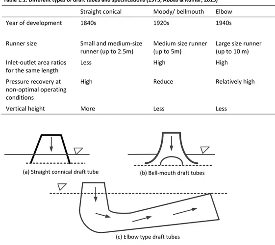
Different types of draft tube and their specifications are presented in Table 1.1 and a schematic diagram is shown in Figure 1.3 (Abbas & Kumar, 2015). Elbow draft tubes are widely used since they require less excavation. They consist of a cylindrical cone, an elbow and a straight diffuser. For a draft tube with outlet width larger than 10 to 12 m, central wall (piers) is usually necessary (Andersson et.al, 2008). Figure 1.4 shows a schematic view of typical Swedish draft tubes with the central wall where also there is an empty space between the draft tube roof and the rock tunnel above, which is filled with water during operation.

Table 1.1: Different types of draft tubes and specifications (1973, Abbas & Kumar, 2015)

Straight conical Moody/ bellmouth Elbow

Year of development 1840s 1920s 1940s

Runner size Small and medium-size

runner (up to 2.5m) Medium size runner (up to 5m) Large size runner (up to 10 m) Inlet-outlet area ratios

for the same length Less High High

Pressure recovery at non-optimal operating conditions

High Reduce Relatively high

Vertical height More Less Less

(a) Straight connical draft tube (b) Bell-mouth draft tubes

(c) Elbow type draft tubes

(12)

Figure 1.4: Elbow draft tube with the central wall (Andersson et.al, 2008)

High flow rates in large dimensions cause the fluid motion in curved draft tubes to be highly turbulent. The outflow from the runner can have more or less swirl depending on the operating condition, and this will affect the performance of the draft tube. At optimal operating conditions this swirl suppresses the boundary layer thickness in the draft tube cone and causes it to operate with full flow across the entire cross-section. Hence, separation is delayed, and the draft tube

performance is increased. The larger amount of swirl, a vortex breakdown will be present due to hydraulic instabilities. The vortex core, located underneath the centre of the runner, reduces the cross-sectional area and thereby is also the draft tube performance decreased due to the higher velocities. The presence of a vortex rope will moreover give rise to large pressure fluctuations which can cause structural damage and flow separation (Marjavaara, 2006).

In the cone, which generally is a straight-conical diffuser, the flow decelerates, and the pressure increases. Any occurrence of severe separation will drastically reduce the draft tube performance and cause damaging pressure fluctuations. Most of the pressure recovery is furthermore obtained in this part of the fluid domain. The primary function of the elbow is to turn the flow from the vertical to the horizontal direction with a minimum loss of energy. The elbow has usually a converging cross-section to avoid separation on its inner section due to the centrifugal forces induced to the flow by the elbow curvature. The outflow diffuser also recovers a part of the kinetic energy, but to a smaller extent than the initial cone, as the velocity at the inlet section of the diffuser is considerably reduced. In addition, the flow in the diffuser is influenced by the flow characteristics at the exit of the elbow, (Gubin, 1973; Amiri et.al., 2016).

Experimental and numerical investigation on the draft tube with a central wall indicated that the central wall strongly affects the flow. The flow is distributed between the two channels of the draft tube which creates a pressure difference between both channels. In another word, it creates a force on the central wall. This force may fluctuate with a frequency related to the runner frequency fr , (Mauri,

(13)

11

1.2 PRINCIPAL OF DRAFT TUBE

A reaction turbine always runs completely filled with the working fluid. The tube that connects the end of the runner to the tailrace is known as a draft tube and should completely be filled with the working fluid flowing through it. The kinetic energy of the fluid finally discharged into the tailrace is wasted. A draft tube is made divergent so as to reduce the velocity at the outlet to a minimum. Therefore, a draft tube is basically a diffuser and should be designed properly to prevent the flow separation from the wall and to reduce accordingly the loss of energy in the tube (Som &Biswas, 2008).

The role of the draft tube can be described by considering the energetic balance ΔE between sections 1 and II with and without the draft tube (see Figure 1.3):

Figure 1.3: Schematic of a draft tube (Mauri, 2002)

(

) (

)

ρ

∆ = ∆ + ∆ + ∆ =2 − + − + 12 1 1 1 1 1 2 II a 2 c E g z p c g z z p p (1.1)

where g is the gravitational acceleration, z the geostatic height, p the pressure, c the mean velocity and pa the atmospheric pressure. The mean velocity at position II is

considered negligible (large surface). The energetic balance between sections 1-I and I-II can be written as follows:

ρ

− + + = + + + ∆ 1 2 2 1 1 1 ₂ ₂ I I I I loss p c p c gz gz E _(1.2)

ρ

− + + 2 = + + ∆ 2 I II a I I I II loss p p c gz gz E _(1.3)

where the losses due to the sudden change in the section between I and II can be

estimated as ∆ − =

(

−

)

=

2 ₂

2 2

I II

loss I II I

E c c c . Without the draft tube p1 = pa so that

Equation (1.1) becomes: 1

II I

(14)

(

)

∆ = − + 21 1 ₂ without II c E g z z (1.4) − ∆ = + ∆ 1 2 2 I I with loss c E E (1.5) The energetic gain due to the diffuser is, therefore:

(

)

− − ∆ − ∆ = − + − ∆ 1 2 2 1 1 ₂ I I

without with II loss

c c

E E g z z E

(1.6)

The draft tube allows the recovery of a part of the kinetic energy between runner outlet and free surface and the level difference.

1.3 CRACK ON DRAFT TUBES CENTRAL WALL

Several hydropower units in Sweden have a draft tube with the central wall. For one major facility cracks on the central wall of draft tubes were detected at first part of the wall, between roof and wall, see Figure 1.6. To fix the problem, concrete was injected through the cracks and a support wall was constructed as an

extension of the wall up to the rock. Finally, a failure of the most upstream part of the wall occurred with ruptured reinforcement and parts of the wall came loose but remained in position.

Figure 1.6: Example of failed contact between central wall and roof

To find out the reasons for the continued crack propagation, model tests were performed at the Hydraulic Machinery Laboratory of Vattenfall Research and Development, Älvkarleby, Sweden (Andersson et.al, 2008). An adjustable draft tube central wall with several pressure holes was used to estimate the load acting on the central wall. The results indicated a significant difference in pressure between both channels due to an uneven flow. At part load the pressure was considerably higher on one side of the central wall, the pressure difference was about 1.5-3 kPa. The pressure difference decreases with increased flow and change high-pressure side at full load. The tests did not indicate any operating point that would cause direct failure of the wall, but possible fatigue problems.

(15)

13

2 Measurements

In one of the Vattenfall facilities with a large, centre wall supported (pier), draft tube, a long-term measurement of pressures and strains on the centre wall and roof have been performed. The monitoring was performed during the period May 2010 to February 2011. This chapter contains a compilation of measurements set-up and calculations. In the first section descriptions of the sensor positions for the draft tube are given, followed by a section that demonstrates the calculation of the pressure from the acquired data. The results from these calculations are used for finite element model, see Chapter6.

2.1 MONITORING SET-UP

A description of the system is done in a Vattenfall report (Holmström, 2010) but a general description of the set-up can be seen in Figure 2.1 and Figure 2.2. To measure the pressure difference across the central wall, a total of four pressure sensors were placed. The sensors were mounted on each side of the central wall with distances of 4 meters from the upstream end of the wall and at the same distance from the draft tube gate and at the centre of the wall. To measure the differential pressure across the draft tube roof, mainly during filling from an empty draft tube, a hole was drilled through the ceiling about 6.5 meters from the upstream end of the wall. All boreholes were sealed with joint foam to prevent pressure equalization in the measurement points.

As illustrated in Figure 2.1, the position of the sensors is P1 at upstream/left side of the wall, P2 at downstream/left side of the wall, P3 at upstream/right side of the wall, P4 at downstream/right side of the wall and P5 at roof/right side of draft tube. It should be noted that sensors P1 and P3 unfortunately failed during the monitoring campaign.

To measure the concrete structure's response to variations in the water pressure, 10 strain gauges have been placed in the right section of the draft tube, central wall and roof of the draft tube. Four strain gauges were mounted on the central wall , as well as six sensors in the roof to follow any deformation of the draft tube structure under load. To measure the change of crack width in the crack between the roof and central wall, a crack-mouth opening gauge was mounted. This gauge failed directly after filling the draft tube. The strain gauges on the central wall located along the draft tube from upstream to downstream are denominated as H1, H3, H10 and H2, respectively, see Figure 2.1. The strain gauges on the roof and along the draft tube from upstream to downstream are denominated as H4, H6, H8 and H9, respectively, see Figure 2.2. Two strain gauges have also been placed on the roof and across the draft tube, H5 and H7 but the former failed from the beginning. The strain gauges were installed on a dog bone shape plate with three different lengths: 300 mm, 160 mm and 132 mm for stain gauges H1-H4, H5-H8 and H9-H10, respectively. The direction of dog bones plates has been shown in Figures 2.1 and 2.2.

(16)

4.0 m 5.0 m 4.0 m 1.8 m 3.15 m 3.15 m 3.15 m 1.8 m +189.26 +191.2 H1 H9 H10 H2 P3 +192.42 (P1) +192.12 (P2) +194.12 P4 +193.74 P5 +196.6

Borehole from the rock above empty space

b1

Figure 2.1: Sensor position in right-hand draft tube central wall and roof (H: strain gauges, P: pressure sensors and b1: crack-opening meter) (Holmström, 2010).

H4 H6 _H8 _H3 H5 H7 1.8 m 3.15 m 3.15 m 3.0 m 2.0 m 3. 7m 1. 8m

Borehole through the draft tube’s roof Borehole from the rock above empty

space

Draft tube’s sluice for the right channel

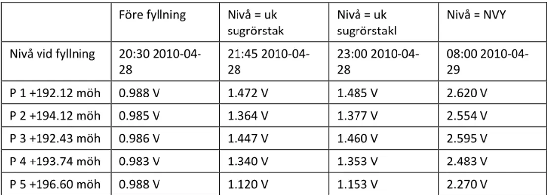
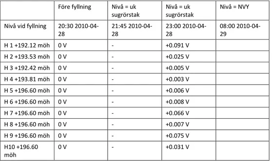
Figure 2.2: Sensor position on the right-hand side of the draft tube roof (H: strain gauges) (Holmström, 2010). Tables 2.1 and 2.3 shows measurements during filling the draft tube. It should be noted that downstream level was +212.96 masl (metres above sea level) during filling the draft tube. During this period the signal from the different sensors was read manually using a Fluke multimeter. As seen in these Tables, sensors had an offset error (before filling draft tube) which has been normalized to zero in Tables 2.2 and 2.4.

(17)

15 Före fyllning Nivå = uk

sugrörstak Nivå = uk sugrörstakl Nivå = NVY Nivå vid fyllning 20:30

2010-04-28 21:45 2010-04-28 23:00 2010-04-28 08:00 2010-04-29 P 1 +192.12 möh 0.988 V 1.472 V 1.485 V 2.620 V P 2 +194.12 möh 0.985 V 1.364 V 1.377 V 2.554 V P 3 +192.43 möh 0.986 V 1.447 V 1.460 V 2.595 V P 4 +193.74 möh 0.983 V 1.340 V 1.353 V 2.483 V P 5 +196.60 möh 0.988 V 1.120 V 1.153 V 2.270 V

Table 2.2: Recalculated values normalized to zero meters of waterpressure before filling (Holmström, 2010) (in Swedish)

Före fyllning Nivå = uk

sugrörstak Nivå = uk sugrörstak Nivå = NVY Nivå vid fyllning 20:30

2010-04-28 21:45 2010-04-28 23:00 2010-04-28 08:00 2010-04-29 P 1 +192.12 möh 0 mvp 6.18 mvp 6.35 mvp 20.84 mvp P 2 +194.12 möh 0 mvp 4.84 mvp 5.00 mvp 19.43 mvp P 3 +192.43 möh 0 mvp 5.89 mvp 6.05 mvp 20.54 mvp P 4 +193.74 möh 0 mvp 4.56 mvp 4.72 mvp 19.15 mvp P 5 +196.60 möh 0 mvp 1.69 mvp 2.11 mvp 16.36 mvp

Table 2.3: Readings on multimeters (Holmström, 2010) (in Swedish)

sugrörstak Nivå = uk sugrörstakl Nivå = NVY Nivå vid fyllning 20:30

2010-04-28 21:45 2010-04-28 23:00 2010-04-28 08:00 2010-04-29 H 1 +192.12 möh -1.178 V - -1.087 V -1.056 V H 2 +193.53 möh 0.034 V - 0.059 V 0.082 V H 3 +192.42 möh -0.712 V - -0.707 V -0.691 V H 4 +193.81 möh -1.153 V - -1.150 V -1.142 V H 5 +196.60 möh -1.172 V - -1.166 V -1.186 V H 6 +196.60 möh -1.174 V - -1.166 V -1.126 V H 7 +196.60 möh -1.009 V - -0.943 V -0.877V* H 8 +196.60 möh -0.031 V - -0.024 V -0.017V* H 9 +196.60 möh -0.766 V - -0.691 V -0.671 V H10 +196.60 möh -0.544 V - -0.544 V -0.557 V

(18)

Table 2.4: The voltages normalized to 0 V before filling (Holmström, 2010)

sugrörstak Nivå = uk sugrörstak Nivå = NVY Nivå vid fyllning 20:30

2010-04-28 21:45 2010-04-28 23:00 2010-04-28 08:00 2010-04-29 H 1 +192.12 möh 0 V - +0.091 V H 2 +193.53 möh 0 V - +0.025 V H 3 +192.42 möh 0 V - +0.005 V H 4 +193.81 möh 0 V - +0.003 V H 5 +196.60 möh 0 V - +0.006 V H 6 +196.60 möh 0 V - +0.008 V H 7 +196.60 möh 0 V - +0.066 V H 8 +196.60 möh 0 V - +0.007 V H 9 +196.60 möh 0 V - +0.075 V H10 +196.60 möh 0 V - +0.031 V

2.2 PRESSURE AND STRAIN DATA INTERPRETATION

Pressure sensors measured total/absolute pressure which contains both effects from static and operational pressure. In mathematical form it can be written as:

ρ

+ 2 = ₀

2

s V

P P (2.1)

Where

ρ

V

2

is called the dynamic pressure, Ps the static pressure, and P0 the

total pressure (Nakayama & Boucher, 1999).

Bernoulli equation is applied to the location of the pressure sensor (point 1) and downstream reading point (point 2), see Figure 2.3:

ρ + + =ρ + + + 2 2 1 1 2 2 1 2 2 2 l P V _Z P V _{Z h} g g g g _(2.2)

Where

h

_lis head loss due to friction between two points. If we consider small friction loss and also the small value of

V

22

2 g

, with considering atmospheric

pressure at downstream and P0 as a total pressure at sensor position (point 1), the

Bernoulli equation will be:

ρ

0 + 1= + +0 0 2 P _Z _Z g (2.3)

(

)

ρ

= − 0 2 1 P Z Z g (2.4)

(19)

17

For a condition that there is no operation, the sensors show hydrostatic pressure, i.e. the pressure due to elevation difference between sensor position and

downstream level. Down stream reading 1 Sensor reading 2 Z1 Z2

Figure 2.3: Pressure measurement

A linear relationship is used to normalize offset error of readings to zero and converting the voltage to mvp (=10 kPa) according to Table 2.1-2.2. Figure 2.4 shows a linear relationship that used for example for sensor P2.

Figure 2.4: A linear relationship used for sensor P2 for converting the voltage to mvp and normalizing offset error

For strain measurement, the zero reading is considered for the case when the draft tube was filled with water (2010-04-29 08:00), see Table 2.3. In this way, the offset error before filling the draft tube and effect for when the draft tube was partly filled is removed. According to the report (Holmström, 2010), 1V was equal to 100 µstrain. For example, for sensor H1, the measurement is corrected as:

= + × 1 ( 1.056) 0.0001 H reading _(2.5) 0.5 1 1.5 2 2.5 3 Voltage (V) 0 5 10 15 20 Pressure (mvp) y = 12.384*x - 12.198 data1 linear

(20)

3 Unit operation measurements

The measurements were divided into two parts; the operation unit measurements and the acquired reading from the sensors and strain gauges. In this chapter, the output effect that was generated from hydropower is presented. In order to see the patterns in the draft tube behaviour regarding load and response, the unit

operational conditions have been considered; normal operation, continuous operation and start and stop events.

3.1 NORMAL OPERATION

It is nowadays common to see turbines being operated over the whole range, with many start/stops, instead of continuous close to peak operation as in the former days. Measurement of unit operation for one year indicated that for normal operation the unit production in daytime is almost between 80-130 MW, see Figure 3.1. It should be noted that the capacity of the unit is 150 MW, but it was restricted to operate not more than 130 MW. It can be seen from Figure 3.1 that the unit had been stopped for a certain time during the summer time; i.e. from July 05 at 01:00 to July 12 at 17:00. Figure 3.2 -3.3 show the unit operation and downstream level as moving average for ten months.

As an example, Figure 3.4 shows normal operation with producing the power of almost 120 MW during daytime for one week. It can be seen also that the operation of the unit starts in the morning for almost 17 hours and stops in the evening.

(21)

19

Figure 3.1: Unit operation during one-year measurement

Jun 2010 Jul 2010 Aug 2010 Sep 2010 Oct 2010 Nov 2010 Dec 2010 Jan 2011 Feb 2011

Date 0 30 60 90 120 Unit operation, MW Jun 13 at 00:00

(22)

Figure 3.2 Unit operation as moving average for ten months.

(23)

21

Figure 3.4: Normal operation with producing power almost 120 MW during daytime for one week

3.2 CONTINUOUS OPERATION

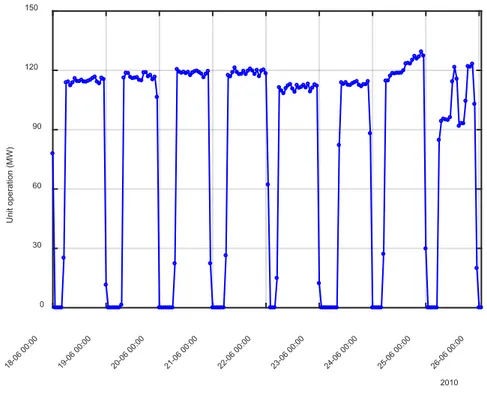
For continuous operation, the unit operates between almost 85 to 130 MW during daytime and nighttime, see Figure 3.1. Figure 3.5 indicates a continuous operation for one week in May-June. As seen in this figure, there are almost no major unit operation fluctuations in production.

18-06 00:00 19-06 00:00 20-06 00:00 21-06 00:00 22-06 00:00 23-06 00:00 24-06 00:00 25-06 00:00 26-06 00:00 2010 0 30 60 90 120 150 Unit operation (MW)

(24)

Figure 3.5: Continuous operation with producing power between 90-130 MW for one week

3.3 START AND STOP EVENTS

The sequence of start and stop during the daytime is illustrated in Figure 3.6. It can be seen in this figure that the stop times are commonly during night-time, but also some at day-time. These sharp starts/stops during day-time can be due to some problems in unit operation.

Figure 3.6: Normal and quick start and stops, for one week

29-05 00:00 30-05 00:00 31-05 00:00 1-06 00:00 2-06 00:00 3-06 00:00 4-06 00:00 5-06 00:00 date(day-month hour) 2010 0 30 60 90 120 150 Unit operation (MW) 10-06 00:00 11-06 00:00 12-06 00:00 13-06 00:00 14-06 00:00 15-06 00:00 16-06 00:00 17-06 00:00 18-06 00:00 2010 0 30 60 90 120 150 Unit opertaion (MW) Day-time stop

(25)

23

4 Pressure measurements

Pressure sensors are installed on the draft tube central wall and roof; to measure the dynamic pressure due to the water which is being finally discharged from the turbine. Depending on the operation unit, the pressure range could be very small. Generally speaking, if the pressure of a system is below or equal to its hydrostatic pressure, the unit is most likely not to operate at all. If the pressure of a system is above its hydrostatic pressure, it operates. The pressure has been measured during one minute for every hour which the mean value of the measurements is

considered and presented as a measured pressure for each hour. Furthermore, 15 minutes measurements also have been done for some stop/start-sequences and fluctuations. The sampling frequency is 100 Hz for all measurements.

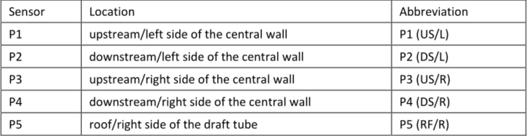
In this chapter, the pressures measurements have been presented for two weeks, 24 hours, 15 minutes and 1 minute. Table 4.1 shows abbreviations that have been used in this report to describe pressure sensors position.

Table 4.1: Abbreviation for pressure sensors on the central wall and roof of the draft tube (see also Figure 2.1 and 2.2).

Sensor Location Abbreviation

P1 upstream/left side of the central wall P1 (US/L) P2 downstream/left side of the central wall P2 (DS/L) P3 upstream/right side of the central wall P3 (US/R) P4 downstream/right side of the central wall P4 (DS/R)

P5 roof/right side of the draft tube P5 (RF/R)

The pressure measurements of all five sensors are shown in Figure 4.1. The

pressure measurements from 28th_{May 2010 to 28}th_{February 2011 were recorded. It}

can be seen that P1 was no longer working in the early stage of measurements on 13th June at 00:00 when the first stop event occurred, i.e. see Figure 2.1 (a). The

cause of such failure may occur due to the connectors were broken, or the cable insulation was damaged because of the fluctuation of the water during the start of the operation unit. Whereas, P3 failed during the stop event of the unit on 10th_July

at 00:00 but in some periods the reading could be considered for example during 19th to 25th January , see Figure 4.1(c). It can also be seen that P2, P4 and P5 have the

same behaviour pattern with minor differences. By excluding P1 and P3, Figure 4.2 shows the minor differences in the measurements of P2, P4 and P5.

(26)

(a)

(b)

(c)

Figure 4.1: Pressure measurement during one year for (a) P1 (US/L), (b) P2 (DS/L), (c) P3 (US/R), (d) P4 (DS/R) and (e) P5 (RF/R).

May 2010 Jun 2010 Jul 2010 Aug 2010 Sep 2010 Oct 2010 Nov 2010 Dec 2010 Jan 2011 Feb 2011 Mar 2011

-200 -100 0 100 200 300 400 500 Pressure (kPa) P1(US/L)

Ti th 0 50 100 150 200 250 Pressure (kPa) P2(DS/L)

Time, month-year -200 0 200 400 600 Pressure (kPa) P3(US/R)

(27)

25

(d)

(e)

(Cont.) Figure 4.1: Pressure measurement during one year for (a) P1 (US/L), (b) P2(DS/L), (c) P3 (US/R), (d) P4 (DS/R) and (e) P5 (RF/R).

Figure 4.2: Pressure measurement during one year for P2 (DS/L), P4 (DS/R) and P5 (RF/R).

Time, month-year 0 50 100 150 200 250 Pressure (kPa) P4 (DS/R)

Time, month-year 0 50 100 150 200 250 Pressure (kPa) P5 (RF/R)

Time, month-year 20 100 150 170 190 210 240 Pressure (kPa) P2(DS/L) P4(DS/R) P5(RF/R)

(28)

The pressure difference along and across the central wall is also calculated from pressure measurement. The pressure due to elevation difference between sensors is removed to calculate pure pressure difference along the central wall and across the central wall. Equations 4.1 and 4.2 show calculation of pressure difference across the central wall at upstream and downstream of the wall, respectively. Equations 4.3 and 4.4 show calculation of pressure difference along the central wall at right and left the side of the central wall, respectively.

ρ ∆P ACRS US( / ) ( 3 0.31 )= P + g P− 1 _(4.1) ρ ∆P ACRS DS( / ) ( 4 0.38= P − g)−P2 _(4.2) ρ ∆P ALG R( / ) ( 3 1.31 )= P − g −P4 _(4.3) ρ ∆P ALG( / L) ( 1 2 )= P − g −P2 _(4.4)

However, the pressure measurements of five sensors for two weeks form 29th_May

at 00:00 until 13th June at 00:00 are shown in Figure 4.3. In this period, all five

sensors work very well. Also, it can be seen that the measured pressure follows the unit operational pattern.

29-05 00:00 1-06 00:00 4-06 00:00 7-06 00:00 10-06 00:00 13-06 00:00 0 30 60 90 120 150 Unit operation (MW) 29-05 00:00 1-06 00:00 4-06 00:00 7-06 00:00 10-06 00:00 13-06 00:00 Time(day-month hour) 2010 150 170 190 210 230 250 Pressure(kPa) P1(US/L) P2(DS/L) P3(US/R) P4(DS/R) P5(RF/R)

(29)

27

The variation of the pressure across the central wall at the downstream and upstream sides of the draft tube can be calculated by using Eq. 4.1-4.2 for the same period from 29th_{May at 00:00 to 13}th_{June at 00:00 and is shown in Figure 4.4 (b).}

The variation of the pressure along the central wall at right and left sides of the central wall are calculated by using Eq. 4.3-4.4 for the same period and illustrated in Figure 4.4 (c).

Figure 4.4: The variation of the pressure during (a) unit operation, (b) across and (c) along the central wall for two weeks. 29-05 00:00 1-06 00:00 4-06 00:00 7-06 00:00 10-06 00:00 13-06 00:00 0 30 60 90 120 150 Unit operation (MW) 29-05 00:00 1-06 00:00 4-06 00:00 7-06 00:00 10-06 00:00 -6 -4 -2 0 2 4 6 8 Pressure(kPa) P (ALG/R) P (ALG/L) 29-05 00:00 1-06 00:00 4-06 00:00 7-06 00:00 10-06 00:00

Time (day-month hour) 2010

-2 0 2 4 6 8 10 12 Pressure(kPa) P (ACRS/DS) P (ACRS/US) (a) (b) (c)

(30)

It can be seen in Figure 4.4 that a drop of the output of 40 MW gives a relative increase of the pressure with approximately four kPa on the upstream position, whereas this reduction gives a decrease of the pressure on the right-hand side with approximately six kPa. A higher relative difference in pressure across the wall can be observed in the downstream position due to even lower values on left-hand side downstream. For one-month measurements, the variation of the pressure of only three sensor P2, P3 and P4 can be achieved by excluding P1 and illustrated in Figure 4.5 (b). Also, the variations of the pressure across the central wall at the downstream side and along the central wall at right side of the central wall are shown in Figure 4.5 (c).

29-05 00:00 5-06 00:00 12-06 00:00 19-06 00:00 26-06 00:00 3-07 00:00 10-07 00:00 0 30 60 90 120 150 Unit operation (MW) 29-05 00:00 5-06 00:00 12-06 00:00 19-06 00:00 26-06 00:00 3-07 00:00 10-07 00:00 0 50 100 150 200 250 Pressure(kPa) _P2(DS/L) P3(US/R) P4(DS/R) 29-05 00:00 5-06 00:00 12-06 00:00 19-06 00:00 26-06 00:00 3-07 00:00 10-07 00:00 2010 -6 -4 -2 0 2 4 6 8 10 12 Pressure(kPa) P (ALG/L) P (ACRS/DS) (a) (b) (c)

(31)

29

4.1 NORMAL OPERATION

In this section, the pressure measurement for normal operation by producing the effect of about 120 MW during daytime is described. Figures 4.6 – 4.7 illustrate a variation of measured pressure for one week and 24 hours, respectively. As shown in these figures, pressure on the right side of the central wall (P3 (US/R) and P4 (DS/R)) is higher than the left side of the central wall (P2 (DS/L)). Pressure on the roof is less than for other sensors. It should be noted that when the unit is off, sensors show hydrostatic pressure. As seen from these figures, the maximum pressure during operation is for sensor P3 (US/R) with a value of almost 230 kPa. The minimum pressure during operation is for sensor P5 (RF/R) with a value of 190.5 kPa.

Figure 4.6: Variation of measured pressure in a week for normal operation by producing the power of about 120 MW. 18-06 00:00 19-06 00:00 20-06 00:00 21-06 00:00 22-06 00:00 23-06 00:00 24-06 00:00 25-06 00:00 26-06 00:00 2010 0 30 60 90 120 150 Unit operation (MW) 18-06 00:00 19-06 00:00 20-06 00:00 21-06 00:00 22-06 00:00 23-06 00:00 24-06 00:00 25-06 00:00 26-06 00:00 Time(day-month hour) 2010 150 170 190 210 230 250 Pressure(kPa) P3(US/R) P4(DS/R) P2(DS/L) P5(RF/R)

(32)

In Figure 4.7 it can be seen there is pressure reduction from daytime (operation of 120 MW) to night-time (no operation) of about 20 kPa in all sensors.

Figure 4.7: Variation of measured pressure in 24 hours for normal operation by producing the effect of about 120 MW.

Figure 4.8 illustrates a variation of pressure across the central wall at the

downstream side of the draft tube (∆P ACRS DS( / )) and along the central wall at

right side of the central wall (∆P ALG R( / )). As seen in this figure during operation of 120 MW the pressure across and along the central wall is almost 11 kPa and -4 kPa, respectively. These values indicate that during operation pressure on the right side of the wall is higher than left side and pressure along the central wall is increasing from upstream to downstream. The figure also highlights that

18-06 18:00 19-06 00:00 19-06 06:00 19-06 12:00 19-06 18:00 0 30 60 90 120 150 Unit operation (MW) 18-06 18:00 19-06 00:00 19-06 06:00 19-06 12:00 19-06 18:00 Time(day-month hour) 2010 150 170 190 210 230 250 Pressure(kPa) P3(US/R) P4(DS/R) P2(DS/L) P5(RF/R)

(33)

31

summarises average pressure measurement during daytime and nighttime for the normal operation.

Figure 4.8: Variation of measured pressure across and along the central wall in a week for normal operation by producing the power of about 120 MW.

Table 4.2: Average of pressure measurement for normal operation, unit kPa

No operation Operation 120 MW P2 (DS/L) 197 211 P3 (US/R) 213 229 P4 (DS/R) 201 219 P5 (RF/R) 172 190 ∆P ACRS DS 7 ( / ) 12 ∆P ALG R ( / ) -0.8 -3.8 18-06 00:00 19-06 00:00 20-06 00:00 21-06 00:00 22-06 00:00 23-06 00:00 24-06 00:00 25-06 00:00 26-06 00:00 0 30 60 90 120 150 Unit operation (MW) 18-06 00:00 19-06 00:00 20-06 00:00 21-06 00:00 22-06 00:00 23-06 00:00 24-06 00:00 25-06 00:00 26-06 00:00

-15 -10 -5 0 5 10 15 Pressure(kPa) P (ALG/L) P (ACRS/DS)

(34)

Figure 4.9 illustrates a linear correlation between pressure measurement and unit operation for one week. As seen from this figure for sensors P2-P5 with increasing effect, the measured pressure is increased.

Figure 4.9: Correlation between pressure measurement and unit operation in a week for normal operation by producing the power of about 120 MW during daytime

Figure 4.10 shows a linear correlation between the variation of pressure along/across and unit operation for one week. As illustrated in this figure with increasing effect, pressure variation across the wall and along the wall increase with higher effect.

Figure 4.10: Correlation between variation of pressure along (LEFT) and across (RIGHT) the central wall and unit operation in a week for normal operation with producing the power of about 110 MW during daytime

The pressure measurement during a stop (2011-01-19 22:51) and start (2011-01-20

0 30 60 90 120 150 Unit operation(MW) 150 200 250 Pressure(kPa) y = 0.115*x + 198 P2(DS/L) linear 0 30 60 90 120 150 Unit operation (MW) 150 200 250 Pressure(kPa) y = 0.129*x + 214 P3(US/R) linear 0 30 60 90 120 150 Unit operation (MW) 150 200 250 Pressure(kPa) y = 0.151*x + 202 P4(DS/R) linear 0 30 60 90 120 150 Unit operation (MW) 150 200 250 Pressure(kPa) y = 0.15*x + 173 P5(RF/R) linear 0 50 100 150 Unit operation (MW) -15 -10 -5 0 5 10 15 Pressure(kPa) y = - 0.0217*x - 0.921 P (ALG/R) linear 0 50 100 150 Unit operation (MW) -15 -10 -5 0 5 10 15 Pressure(kPa) y = 0.036*x + 6.76 P (ACRS/DS) linear

(35)

33

during the stop the unit, the reducing effect from 75 MW to 0, at time 22:51 has been shown in Figure 4.11. This measurement should be compared with 1 min measurement at time 23:00 see Table 4.3. As seen in this Figure pressure measured after 15 min is close to the values measured in 1 min at time 23:00. The same goes for the pressure difference along and across the central wall, see Figure 4.12. From the pressure measurements, it is obvious that the changes in total pressure (20-25 kPa the first minutes) from reducing the unit effect is overruling any differential pressures along and across the wall (less than two kPa).

Table 4.3: Average measured pressure at time 22.00 and 23:00 from 1 min reading (unit kPa) P3(US/R) P4(DS/R) P2(DS/L) P5(RF/R) ∆_{P ACRS DS ∆ (}( / ) _{P ALG R}/ ) 75 MW (22:00) 230.7 221.1 213.2 192.6 4.099 -3.493 0 MW (23:00) 216.9 201.9 200.9 176.3 0.2537 -1.161

Figure 4.11: Variation of measured pressure in 15 min for normal operation during stop-reducing effect from 75 MW to 0 (2011-01-19 22:51)

Figure 4.12: Variation of pressure along and across the central wall in 15 min for normal operation during stop-reducing effect from 75 MW to 0 (2011-01-19 22:51)

0 5 10 15 Time(min) -6 -4 -2 0 2 4 6 Pressure(kPa) P (ALG/R) 0 5 10 15 Time(min) -6 -4 -2 0 2 4 6 Pressure(kPa) P (ACRS/DS)

(36)

Figure 4.13 illustrates 15 min measurement during a start at time 06:49, increasing effect from 25 MW to 110 MW. This measurement is compared with measured pressure in 1 min at 07:00, see Table 4.4. The comparison indicates that the last peak in pressure measurement of Figure 4.7 is close to the measured pressure at time 07:00 from 1 min reading. The same goes for pressure along and across the central wall, see Figure 4.14. The reason is that in the last 5 min measurement the unit operates with the production of 110 MW. It can be seen that the change in total pressure when increasing the unit operation can be as large as 30-35 kPa and the increase in differential pressures are visible after 5 to 10 minutes, but in the same range as during normal operation.

Table 4.4: Average measured pressure at time 06.00 and 07:00 from 1 min reading (unit kPa)

P3 (US/R) P4 (DS/R) P2 (DS/L) P5 (RF/R) ∆P ACRS DS( / ) ∆P ALG R ( / ) 25 MW (06:00) 212.7 200.8 196.8 172.2 0.1399 -1.149 110 MW (07:00) 228.4 218.7 210.9 190.1 4.017 -3.433

Figure 4.13: Variation of measured pressure in 15 min for normal operation during start-increasing effect from 25 MW to 110 MW (2011-01-20 06:49)

(37)

35

Figure 4.14: Variation of pressure along and across the central wall in 15 min for normal operation during start-increasing effect from 25 MW to 110 MW (2011-01-20 06:49).

4.2 CONTINUOUS OPERATION

In this section, the pressure measurement for continuous operation by producing power between 85-130 MW is described. Figures 4.15 and 4.16 show variation of measured pressure for one week and 24 hours, respectively. As seen from this Figures, pressure measurement follows unit operation pattern. Furthermore, pressure on the right side of the central wall is higher than the left side of the central wall. Pressure on the roof is less than others.

0 5 10 15 Time(min) -6 -4 -2 0 2 4 Pressure(kPa) P (ALG/R) 0 5 10 15 Time(min) -6 -4 -2 0 2 4 Pressure(kPa) P (ACRS/DS)

(38)

Figure 4.15: Variation of measured pressure in a week for continuous operation with producing power between 85-130 MW (see Table 4.1 for pressure sensor abbreviation).

29-05 00:00 30-05 00:00 31-05 00:00 1-06 00:00 2-06 00:00 3-06 00:00 4-06 00:00 5-06 00:00 0 30 60 90 120 150 Unit operation (MW) 29-05 00:00 30-05 00:00 31-05 00:00 1-06 00:00 2-06 00:00 3-06 00:00 4-06 00:00 5-06 00:00

150 170 190 210 230 250 Pressure(kPa) P3(US/R) P4(DS/R) P2(DS/L) P5(RF/R)

(39)

37

Figure 4.16: Variation of measured pressure in 24 hours for continuous operation with producing power between 85-130 MW

The variations of pressure across the central wall and along the central wall for continuous operation are demonstrated in Figure 4.17. As seen from this figure average pressure measurement across the central wall during 130 MW and 85 MW operations is 10.8 kPa and 8.1 kPa, respectively. Furthermore, average pressure measurement along the central wall during operation of 130 MW and 85 MW is -2.3 kPa and -1.85 kPa, respectively. The minus sign indicates increasing pressure along the central wall from upstream to downstream (this shows the effect of the draft tube, increasing static pressure along the draft tube).

1-06 12:00 1-06 06:00 2-06 12:00 2-06 06:00 2-06 12:00 2010 0 30 60 90 120 Unit operation,(MW) 1-06 12:00 1-06 18:00 2-06 00:00 2-06 06:00 2-06 12:00

150 170 190 210 230 250 Pressure(kPa) P3(US/R) P4(DS/R) P2(DS/L) P5(RF/R)

(40)

Figure 4.17: Variation of measured pressure across and along the central wall in a week for continuous operation with producing power between 85-130 MW.

However, the average pressure measurement during operation of 130 MW and 80 MW are summarised in Table 4.4.

Table 4.4: Average of pressure measurement for continuous operation, unit kPa

130 MW 85 MW P3 (US/R) 226.7 223.45 P4 (DS/R) 216.37 213.46 P2 (DS/L) 209.5 207.45 P5 (RF/R) 187.88 184.94 ∆P ACRS DS ( / ) 10.8 8.1 ∆P ALG R ( / ) -2.3 -1.9 29-05 00:00 30-05 00:00 31-05 00:00 1-06 00:00 2-06 00:00 3-06 00:00 4-06 00:00 5-06 00:00 0 30 60 90 120 150 Unit operation (MW) 29-05 12:00 30-05 12:00 31-05 12:00 1-06 12:00 2-06 12:00 3-06 12:00 4-06 12:00 5-06 12:00

-15 -10 -5 0 5 10 15 Pressure(kPa) P (ACRS/DS) P(ALG/R)

(41)

39

A linear correlation between pressure measurement and unit operation can be found for one-week occasion and shown in Figure 4.18. As seen from this figure for all sensors with increasing the unit operation power, the measured pressure is increased. Figure 4.19 shows the correlation between unit operation and pressure along and across the central wall. It is observed that with the increasing effect the pressure difference across and along the central wall is increased. The behaviour regarding pressures along and across the wall show a good correlation with the unit operation.

Figure 4.18: Correlation between pressure measurement and unit operation in a week for continuous operation with producing power between 85-130 MW

Figure 4.19: Correlation between variation of pressure along/across the central wall and unit operation in a week for week for continuous operation with producing power between 85-130 MW

0 30 60 90 120 150 Unit operation (MW) 150 200 250 Pressure(kPa) y = 0.238*x + 204 P3(US/R) linear 0 30 60 90 120 150 Unit operation (MW) 150 200 250 Pressure(kPa) y = 0.236*x + 193 P4(DS/R) linear 0 30 60 90 120 150 Unit operation (MW) 150 200 250 Pressure(kPa) y = 0.194*x + 191 P2(DS/L) linear 0 30 60 90 120 150 Unit operation (MW) 150 200 250 Pressure(kPa) y = 0.241*x + 164 P5(RF/R) linear 0 50 100 150 Unit operation (MW) -15 -10 -5 0 5 10 15 Pressure(kPa) y = 0.0424*x + 5.39 P (ACRS/DS) linear 0 50 100 150 Unit operation (MW) -15 -10 -5 0 5 10 15 Pressure(kPa) y = 0.00241*x - 2.81 P (ALG/R) linear

(42)

4.3 FAST START AND STOP EVENTS

The variation of pressure of four sensors during operation with a sharp stop and start was considered in this section and shown in Figure 4.20. As seen from this figure during stopping the unit, pressure goes lower than the hydrostatic pressure (pressure during no operation). For example, the unit was shut down on 14th_June

from 15:00 to 18:00 for unknown reasons, therefore, the unit operation power dropped from 90 MW to 0 MW. The overall behaviour pattern of the measured pressure is about the same as for the normal operation. The sequence of start and stop in daytime on 14th June is shown in Figure 4.21.

Figure 4.20: Variation of measured pressure in a week for normal and quick start and stops 10-06 00:00 11-06 00:00 12-06 00:00 13-06 00:00 14-06 00:00 15-06 00:00 16-06 00:00 17-06 00:00 18-06 00:00 0 30 60 90 120 150 Unit operation (MW) 10-06 00:00 11-06 00:00 12-06 00:00 13-06 00:00 14-06 00:00 15-06 00:00 16-06 00:00 17-06 00:00 18-06 00:00 Time(day-month hour) 2010 150 170 190 210 230 250 Pressure(kPa) P3(US/R) P4(DS/R) P2(DS/L) P5(RF/R)

(43)

41

Figure 4.21: Variation of measured pressure in 24 hours for normal and quick start and stops

Variation of pressure across the central wall has been shown in Figure 4.22. The highest pressure difference across the wall is five kPa during operation of 90 MW. Table 4.5 summarises pressure measurement during a sequence of start/stop. Table 4.5: Average measured pressure for stop and started event (unit: kPa)

90 MW (14:00) 0 MW (15:00) P2 (DS/L) 209 196 P3 (US/R) 226 212 P4 (DS/R) 214 200 P5 (RF/R) 185 170 ∆P ACRS DS ( / ) 17 4 14-06 06:00 14-06 12:00 14-06 18:00 15-06 00:00 0 30 60 90 120 150 Unit operation (MW) 14-06 06:00 14-06 12:00 14-06 18:00 15-06 00:00 Time(day-month hour) 2010 150 170 190 210 230 250 Pressure(kPa) P3(US/R) P4(DS/R) P2(DS/L) P5(RF/R)

(44)

In the following pressure measurement in 15 min during stopping the unit from 8.68 MW and 19.15 MW is shown. It should be noted that pressure measurement during the starting unit is not shown due to insignificant variation in pressure across the central wall. Figure 4.20 shows a variation of measured pressure in 15 min during stop-reducing effect from 8.68 MW to 0 (2010-12-20 10:16). The variation of pressure across the central wall is almost zero, see Figure 4.21.

Figure 4.20: Variation of measured pressure in 15 min during stop-reducing effect from 8.68 MW to 0 (2010-12-20 10:16)

Figure 4.21: Variation of pressure across the central wall in 15 min during stop-reducing effect from 8.68 MW to 0 (2010-12-20 10:16)

Figure 4.22 shows a variation of measured pressure in 15 min during stop-reducing effect from 19.15 MW to 0 (2010-12-20 12:23). It has more pressure fluctuation compared to Figure 4.20. Furthermore, maximum pressure across the central wall is almost four kPa, see Figure 4.23. This must be compared with 1 min

measurement which shows almost zero pressure difference.

0 5 10 15 Time (min) -6 -4 -2 0 2 4 6 Pressure(kPa) P (ACRS/DS)

(45)

43

Figure 4.22: Variation of measured pressure in 15 min during stop-reducing effect from 19.15 MW to 0 (2010-12-20 12:23)

Figure 4.23: Variation of pressure across the central wall in 15 min during stop-reducing effect from 19.15 MW to 0 (2010-12-20 12:23) 0 5 10 15 Time (min) -6 -4 -2 0 2 4 6 Pressure(kPa) P (ACRS/DS)

(46)

5 Strain measurements

In this chapter, the response of the draft tube due to pressure changes induced by the different operational pattern is described. Strain gauges are installed on the draft tubes central wall and roof. The strain has been measured one minute for each hour which means the value of it is considered as a measured strain for each hour.

Furthermore, 15 minutes measurement also has been done for during stop/start and at large fluctuations in operation. In the following, examples of strain measurement corresponding to the operational patterns and pressure

measurement are described. Table 5.1 and 5.2 shows abbreviations that have been used to describe the strain gauges position. See also Figure 2.1 and 2.2 for their position.

Table 5.1: Abbreviations for strain gauges on the right side of the central wall from upstream to downstream (See also Figure 2.1 and 2.2)

H1 Upstream H1 (US/WL)

H9 Upstream, after sensor H1 H9 (USb/WL) H10 Downstream, before sensor H2 H10 (DSb/WL)

H2 Downstream H2 (DS/WL)

Table 5.2: Abbreviations for strain gauges on the roof /right side of the draft tube

H4 Upstream H4 (US/RF)

H6 Upstream, after sensor H4 H6 (USb/RF)

H8 Downstream, before sensor H9 H8 (DSb/RF)

H3 Downstream H3 (DS/RF)

H7 Across the draft tube roof H7 (ACRS/RF)

Figure 5.1-5.3 illustrates pressure measurements of all ten strain gauges during one year starting from 28 May 2010. The measured strain along the right side of the middle wall in the draft tube is presented in Figure 5.1. Whereas, the measured strain under the roof is presented in Figure 5.2-5.3. It can be seen from these figures that after July the measurement of H1-4 and H6-10 had drifted while H5 was failed from the beginning.

This drift can be because of draining draft tube in July and refilling it. In Figure 5.4, the blue curve shows strain measurement. A best-fit curve with red colour

indicates the trend in data. The green curve shows strain measurement after eliminating the trend. Trend removal process has been used for example in signal processing and shock vibration test of concrete to remove rigid body motion of the specimens, see, e.g. Kwan et al. (2002). In Figure 5.5 to 5.7 the corrected strain measurements are shown.

(47)

45

Figure 5.1 Measured strain of H1, H9, H10 and H2 on the right side of the central wall.

Figure 5.2 Measured strain of H4, H6, H8 and H3 along the roof.

Figure 5.3 Measured strain of H7 and H5, across the roof.

Time(day-month hour) 0 2 4 6 8 strain [ 10 -6 ] Strain gauge H1 Strain gauge H9 Strain gauge H10 Strain gauge H2

Time(day-month hour) 0 2 4 6 8 strain [ 10 -6 ] Strain gauge H4 Strain gauge H6 Strain gauge H8 Strain gauge H3

Time(day-month hour) 0 2 4 6 8 strain [ 10 -6 ] Strain gauge H7 Strain gauge H5

(48)

Figure 5.4: Trend removal process from strain measurement

Figure 5.5 Corrected measured strain of H1, H9, H10 and H2 on the right side of the central wall.

Figure 5.6 Corrected measured strain of H4, H8, H3 and H6 along the roof.

Jun 2010 Jul 2010 _{Aug 2010} _{Sep 2010} Oct 2010 Nov 2010 Dec 2010 Jan 2011 Feb 2011

date(day-month hour) 0 100 200 300 400 500 strain [ 10 -6 ] H1 Best fitting New H1

Time(day-month hour) 0 0.5 1 1.5 2 strain [ 10 -6 ] Strain gauge H1 Strain gauge H9 Strain gauge H10 Strain gauge H2

Time(day-month hour) 0 0.5 1 1.5 2 strain [ 10 -6 ] Strain gauge H4 Strain gauge H6 Strain gauge H8 Strain gauge H3

(49)

47

Figure 5.7 Corrected measured strain of H7 without H5, across the roof (see Figure 2.2).

5.1 NORMAL OPERATION

In this section, the strain measurement for normal operation by producing the power of about 110 MW during daytime is described. Figure 5.8 illustrates a variation of measured strain on the wall and roof for one week. Comparison between two figures indicates that the general strain level under the roof is higher than the strain on the wall. The maximum strain on the wall is about 94.55e-6 for sensor H1 at the upstream side of the draft tube, and maximum strain on the roof is about 105.22e-6 for sensor H7 across the draft tube.

Time(day-month hour) 0 0.5 1 1.5 2 strain [ 10 -6 ] Strain gauge H7

(50)

(a) (b) 18-06 00:00 19-06 00:00 20-06 00:00 21-06 00:00 22-06 00:00 23-06 00:00 24-06 00:00 25-06 00:00 26-06 00:00 date(day-month hour) 2010 0 30 60 90 120 150 Unit operation (MW) 18-06 00:00 19-06 00:00 20-06 00:00 21-06 00:00 22-06 00:00 23-06 00:00 24-06 00:00 25-06 00:00 26-06 00:00 Time(day-month hour) 2010 150 170 190 210 230 250 Pressure(kPa) P3(US/R) P4(DS/R) P2(DS/L) P5(RF/R) 18-06 00:00 19-06 00:00 20-06 00:00 21-06 00:00 22-06 00:00 23-06 00:00 24-06 00:00 25-06 00:00 26-06 00:00

0 0.5 1 1.5 2 2.5 3 strain [ 10 -6 ] H1(US/WL) H9(USb/WL) H10(DSb/WL) H2(DS/WL)

(51)

49

(d)

Figure 5.8: Normal operation with producing the power of about 110 MW (a) for one week measured pressures (b) and measured strains on the wall (c) and the roof (d).

Figures above also show drifts in strain measurement during start and stop events. To see these changes, a variation of measured strain on the wall and roof is studied for 24 hours, see Figures 5.9. As seen from these figures, the fluctuations in

pressure from changing operation have almost no impact on the strains and no obvious correlation to either pressure or operation. The average measured strain on the wall and roof during daytime and nighttime has been summarized in Tables 5.3 and 5.4, respectively. (a) 18-06 00:00 19-06 00:00 20-06 00:00 21-06 00:00 22-06 00:00 23-06 00:00 24-06 00:00 25-06 00:00 26-06 00:00 date(day-month hour) 2010 0 0.5 1 1.5 2 2.5 3 strain [ 10 -6 ] H4(US/RF) H6(USb/RF) H8(DSb/RF) H3(DS/RF) H7(ACRS/RF) 19-06 12:00 19-06 18:00 20-06 00:00 20-06 06:00 20-06 12:00 2010 0 30 60 90 120 150 Unit operation (MW)

(52)

(b)

(c)

Figure 5.9: Variation of measured strain on (a) the wall and (b) roof in 24 hours for normal operation with producing the power of about 120 MW.

Table 5.3: Average measured strain on the wall during daytime and nighttime for normal operation (µstrain)

H1 (US/WL) H9 (USb/WL) H10 (DSb/WL) H2 (DS/WL) 0 MW (night time) 0.9418 0.5586 0.3994 0.5477 120 MW (daytime) 1.013 0.6028 0.365 0.6192 120 MW to 0 MW 0.0712 0.0442 0.0344 0.0715 19-06 12:00 19-06 18:00 20-06 00:00 20-06 06:00 20-06 12:00 date(day-month hour) 2010 0 0.5 1 1.5 2 2.5 3 strain [ 10 -6 ] H1(US/WL) H2(DS/WL) H9(USb/WL) H10(DSb/WL) 19-06 12:00 19-06 18:00 20-06 00:00 20-06 06:00 20-06 12:00 date(day-month hour) 2010 0 0.5 1 1.5 2 2.5 3 strain [ 10 -6 ] H4(US/RF) H6(USb/RF) H8(DSb/RF) H3(DS/RF) H7(ACRS/RF)

(53)

51 H4 (US/RF) H6 (USb/RF) H8 (DSb/RF) H3 (DS/RF) H7 (ACRS/RF) 0 MW (night time) 1.052 1.242 0.7464 0.2369 1.38 120 MW (daytime) 1.135 1.303 0.8215 0.3167 1.412 120 MW to 0 MW 0.083 0.061 0.0751 0.0798 0.032

Figures 5.10-5.12 show a correlation between pressure and strain measurement on the roof, central wall and across the wall, respectively. Correlation has been shown for the closest strain sensor to the pressure gages.

Figure 5.10: Correlation between pressure and strain measurement on the roof for normal operation with production of 110 MW in a week. Y-axis scale is 0.5 µstrain.

Figure 5.11: Correlation between pressure and strain measurement on the wall for normal operation with production of 110 MW in a week. Y-axis scale is 0.5 µstrain.

150 170 190 210 230 250 Pressure(kPa) 1.2 1.3 1.4 1.5 1.6 1.7 strain [ 10 -6 ] P5(RF/R),H7(ACRS/RF) 150 170 190 210 230 250 Pressure(kPa) 1 1.1 1.2 1.3 1.4 1.5 strain [ 10 -6 ] P5(RF/R),H6(USb/RF) 150 170 190 210 230 250 Pressure(kPa) 0.4 0.5 0.6 0.7 0.8 0.9 strain [ 10 -6 ] P3(US/R),H9(USb/WL) 150 170 190 210 230 250 Pressure(kPa) 0.2 0.3 0.4 0.5 0.6 0.7 strain [ 10 -6 ] P4(DS/R),H10(DSb/WL)

(54)

Figure 5.12: Correlation between pressure across the central wall and strain measurement on the wall for normal operation with production of 110 MW in a week. Y-axis scale is 0.5 µstrain.

15 min measurement during the stop the unit, reducing effect from 75 MW to 0, at time 22:51 has been shown in Figures 5.13 and 5.14 for wall and roof, respectively. As seen from the figures, apart from sensor H7 (ACRS/RF), all sensors have small descending behaviour. This measurement is compared with 1 min reading at time 23:00, see Tables 5.5-5.6. Comparison between 15 min readings and 1 min readings indicates that after almost 10 min of reading the strain values convergence to the values from 1 min reading at time 23:00.

Table 5.5: Average measured strain on the wall at time 22.00 and 23:00 from 1 min reading (µstrain)

H1 (US/WL) H9 (USb/WL) H10 (DSb/WL) H2 (DS/WL) 75 MW (22:00) 0.9388 0.1987 0.3387 0.5291 0 MW (23:00) 0.9627 0.1915 0.34 0.5256

Table 5.6: Average measured strain on the roof at time 22.00 and 23:00 from 1 min reading (µstrain)

H4 (US/RF) H6 (USb/RF) H8 (DSb/RF) H3 (DS/RF) H7 (ACRS/RF) 75 MW (22:00) 1.051 1.17 0.6942 0.5156 1.375 0 MW (23:00) 1.03 1.16 0.682 0.5211 1.366 6 8 10 12 Pressure(kPa) 0.2 0.3 0.4 0.5 0.6 0.7 strain [ 10 -6 ] P(ACRS/DS),H10(DSb/WL)

(55)

53

Figure 5.13: Variation of measured strain on the wall in 15 min for normal operation during stop- reducing effect from 75 MW to 0 (2011-01-19 22:51). Y-axis scale is 0.01 µstrain.

0 5 10 15 Time(min) 0.965 0.967 0.969 0.971 0.973 Strain [ 10 -6 ] H1(US/WL) 0 5 10 15 Time(min) 0.54 0.542 0.544 0.546 0.548 Strain [ 10 -6 ] H9(USb/WL) 0 5 10 15 Time(min) 0.34 0.342 0.344 0.346 0.348 0.35 Strain [ 10 -6 ] H10(DSb/WL) 0 5 10 15 Time(min) 0.525 0.527 0.529 0.531 0.533 0.535 Strain [ 10 -6 ] H2(DS/WL)

(56)

Figure 5.14: Variation of measured strain on the roof in 15 min for normal operation during stop- reducing effect from 75 MW to 0 (2011-01-19 22:51). Y-axis scale is 0.03 µstrain.

Figures 5.15-16 shows a variation of measured strain in 15 min for normal

operation during start- increasing effect from 25 MW to 110 MW (2011-01-20 06:49) on the wall and roof, respectively. It is seen from figures that except sensor H1 (US/WL) and H9 (DS/RF), all sensors have a small ascending behaviour. All sensors convergence to the value of strain measurement from 1 min readings at time 07:00 when there are 110 MW operations, see Tables 5.7-5.8.

0 5 10 15 Time (min) 1.038 1.04 1.042 1.044 1.046 Strain [ 10 -6 ] H4(US/RF) 0 5 10 15 Time (min) 1.16 1.162 1.164 1.166 1.168 1.17 Strain [ 10 -6 ] H6(USb/RF) 0 5 10 15 Time (min) 0.68 0.682 0.684 0.686 0.688 0.69 Strain [ 10 -6 ] H8(DSb/RF) 0 5 10 15 Time (min) 0.17 0.172 0.174 0.176 0.178 0.18 Strain [ 10 -6 ] H3(DS/RF) 0 5 10 15 Time (min) 1.354 1.356 1.358 1.36 1.362 1.364 Strain [ 10 -6 ] H7(ACRS/RF)