Comparison of Forecasting Models Used by The Swedish Social Insurance Agency.

(1)

MASTER THESIS IN FINANCIAL ENGINEERING

Comparison of Forecasting Models Used by

The Swedish Social Insurance Agency.

by

Ryan Rasoul

(2)

Master thesis in Financial Engineering

Date:

2020-06-05

Project name:

Comparison of forecasting models used by The Swedish Social Insurance Agency.

Author: Ryan Rasoul Supervisor: Dr. Karl Lundengård Reviewer: Dr. Fredrik Jansson Examiner: Dr. Jonas Sjöstrand

(3)

(4)

Acknowledgements

I would like to thank my supervisor Dr. Karl Lundengård for the immense help and support

he extended to me.

Special thanks to the manager of the forecast department at the Swedish Social Insurance

Agency, Axel Arvidsson for his support and trust.

(5)

Abstract

We will compare two different forecasting models with the forecasting model that was used in March 2014 by The Swedish Social Insurance Agency ("Försäkringskassan" in Swedish or "FK") in this degree project. The models are used for forecasting the number of cases. The two models that will be compared with the model used by FK are the Seasonal Exponential Smoothing model (SES) and Auto-Regressive Integrated Moving Average (ARIMA) model. The models will be used to predict case volumes for two types of benefits: General Child Allowance “Barnbidrag” or (BB_ABB), and Pregnancy Benefit

“Graviditetspenning” (GP_ANS).

The results compare the forecast errors at the short time horizon (22) months and at the long-time horizon (70) months for the different types of models. Forecast error is the difference between the actual and the forecast value of case numbers received every month. The ARIMA model used in this degree project for GP_ANS had forecast errors on short and long horizons that are lower than the forecasting model that was used by FK in March 2014. However, the absolute forecast error is lower in the actual used model than in the ARIMA and SES models for pregnancy benefit cases.

The results also show that for BB_ABB the forecast errors were large in all models, but it was the lowest in the actual used model (even the absolute forecast error). This shows that random error due to laws, rules, and community changes is almost impossible to predict. Therefore, it is not feasible to predict the time series with tested models in the long-term. However, that mainly depends on what FK considers as accepted

forecast errors and how those forecasts will be used.

It is important to mention that the implementation of ARIMA differs across different software. The best model in the used software in this degree project SAS (Statistical Analysis System) is not necessarily the best in other software.

(6)

List of Tables

3.1: March 2020 forecast for child allowance case volumes ……… 12

3.2: Historical data for BB_ABB time series ………... 13

3.3: Absolute values of BB_ABB Forecast errors ………... 14

3.4: March 2020 forecast for Pregnancy benefit case volumes ……… 19

3.5: Historical data for GP_ANS time series ……… 19

3.6: Absolute values of GP_ANS Forecast errors ……… 20

4.1: Comparison of BB_ABB Forecast errors for the three models ……... 25

4.2: Comparison of BB_ABB Forecast errors for SES and ARIMA ……... 26

4.3: Comparison of GP_ANS Forecast errors for the three models ……… 28

4.4: Comparison of GP_ANS Forecast errors for SES and ARIMA ……... 29

List of Figures

3.1: Historical data for ABB time series ………... 13

3.2: BB_ABB ARIMA Prediction Error White Noise Probability ………. 16

3.3: BB_ABB ARIMA Prediction Error Correlation ……….. 16

3.4: BB_ABB ARIMA Model and Forecasts……… 16

3.5: BB_ABB ARIMA Prediction Errors………. 16

3.6: BB_ABB SES Prediction Error White Noise Probability ………. 17

3.7: BB_ABB SES Prediction Error Correlation ……….. 17

3.8: BB_ABB SES Model and Forecasts ………... 17

3.9: BB_ABB SES Prediction Errors ……… 17

3.10: BB_ABB White Noise probabilities ………... 18

3.11: BB_ABB Seasonal Decomposition/Adjustment ………. 18

3.12: BB_ABB Series Values ……….. 18

3.13: BB_ABB Correlations ……… 18

3.14: GP_ANS Time Series ………... 19

3.15: GP_ANS ARIMA Prediction Error White Noise Probability ………. 22

3.16: GP_ANS ARIMA Prediction Error Correlation ……….. 22

3.17: GP_ANS ARIMA Model and Forecasts ………. 22

3.18: GP_ANS ARIMA Prediction Errors ………... 22

3.19: GP_ANS SES Prediction Error White Noise Probability ……… 23

3.20: GP_ANS SES Prediction Error Correlation ……… 23

3.21: GP_ANS SES Model and Forecasts ……… 23

3.22: GP_ANS SES Prediction Errors ……….. 23

3.23: GP_ANS White Noise probabilities ……….... 24

3.24: GP_ANS Seasonal Decomposition/Adjustment ……….. 24

3.25: GP_ANS Series Values ………... 24

3.26: GP_ANS Correlations ………. 24

4.1: BB_ABB Absolute Forecast errors for SES model ……….. 26

4.2: BB_ABB Absolute Forecast errors for ARIMA model ……… 27

4.3: BB_ABB Absolute Forecast errors for the actual forecast………….... 27

4.4: Comparison of BB_ABB Forecast errors for the three models ………. 27

4.5: GP_ANS Absolute Forecast errors for SES model……… 29

4.6: GP_ANS Absolute Forecast errors for ARIMA model ……….... 30

4.7: GP_ANS Absolute Forecast errors for the actual forecast ……… 30

(8)

1 Introduction

The Swedish Social Insurance Agency’s role is to administer the areas of the social insurance that provides financial security in the event of illness, disability, and to families with children.

The Analysis and Forecasting Division (AP) at the agency produces forecasts of the development of case volumes for a number of benefits in social insurance. The purpose of the case volume forecasts is to use them as a basis for the agency's operation planning. This means in practice that the forecasts are used in staff and production planning in the distribution of funds within the authority, and as a basis for the forecast for the administrative appropriation.

Case volume forecasts (in Swedish “Ärendevolymsprognoser ” or “ÄVP”) data is a series of numbers of cases that are created in different divisions of FK on a monthly basis, and it's classified in categories and subcategories. The forecasts are made for 27 benefits (including recoveries and re-examinations) with over 100 related case types. They are produced four times a year (March, June, September, and November) and extend forecasting for 4 years ahead. FK publishes on its website the forecasting for the expenses of the social benefits for the coming years but not the forecasting of case volumes [1].

1.1 Forecast basis

The users of the forecasts are asked to pay attention to the definitions of the metrics since for several of the benefits several different metrics are forecasted. The social insurance benefits that AP forecasts vary widely and show different patterns. There is also a wide variation in benefits in terms of how complicated the cases are and in the amount of work required per case.

Forecasts are usually uncertain, and the uncertainty increases with the longer period of the forecasts. Large fluctuations in the flow of cases and a lack of statistical data, for example, with short time series create uncertainty. Changes in regulatory system definitions and management routines also contribute to

uncertainty. AP only produces national forecasts, and the uncertainty in the nationwide forecasts means that the uncertainty increases when these are broken down regionally.

Forecasts from other government agencies are also used as input to the forecast models such as the

population forecast from Statistics Sweden (SCB), and forecasts from the Migration Agency, Employment Service, and The National Institute of Economic Research.

Previous experience of forecasting and a comprehensive grasp of the benefits are of great importance when forecasting. Modern statistical methods are great tools to analyze large quantities of data and make

predictions.

I will attempt to construct multivariate time series models with the aim of forecasting FK case volumes in this degree project. These models will then be compared with the actual forecast made by AP in March 2014 to test their ability to generate accurate forecasts. The primary reason for this multivariate approach is to enable the inclusion of various confidence indicators in the forecasting process. The confidence indicators are generally useful in forecasting the number of cases in the short term.

(9)

2 Theory

2.1 A brief history of time series analysis

The first actual application of autoregressive models to data was by G. U Yule and J. Walker in the 1920s and 1930s [2]. The moving average was introduced during this time to remove periodic fluctuations in the time series, for example, fluctuations due to seasonality. ARMA (Autoregressive Moving Average) models for stationery series were introduced by Herman Wold, but he was unable to derive a likelihood function to enable maximum likelihood (ML) estimation of the parameters. This was accomplished in the year 1970, as in that year the classic book "Time Series Analysis" by G. E. P. Box, G. M. Jenkins, and G.C Reinsel [3] came out. The book contained the whole modeling procedure for individual series: specification,

estimation, diagnostics, and forecasting.

Perhaps nowadays the Box-Jenkins models are the most commonly used, and many techniques for forecasting and seasonal adjustment can be traced to these models. Multivariate ARMA models, for example, VAR (Vector autoregression) models were developed and became popular during the 1980s. In 1956 Robert Goodell Brown suggested the Exponential smoothing in the statistical literature for the first time. Charles C. Holt then expanded this work in 1957 [4]. One of the commonly used formulations which is attributed to Brown is known as “Brown’s simple exponential smoothing”. Holt, Winters, and Brown methods can be seen as a simple application of recursive filtering [5].

2.2 Time Series Modelling of Case Volumes

For modeling purposes, it can be helpful to think of any time series such as case volumes as generated by an unknown data generating process. This process could possibly be extremely complex and include a near-infinite number of parameters. It is in most cases only possible to set up a model that approximates the true process. If the underlying process remains unchanged over time, we can think of every observation in the time series as generated by this process. This can help to fit a model that would seem to be a likely candidate to have generated these observed outcomes. This approximation of the underlying process can then be used for forecasting purposes.

I tested several models in this degree project with SAS, since FK uses this software for its forecasts. I selected the models with the lowest MAPE (Mean Absolute Percentage Error), as this is the most used way of selecting models in AP. The models that had the lowest MAPE were Seasonal Exponential Smoothing and ARIMA for the studied benefits during that period. There were other models that had been rejected such as AR, MA, and ARMA because they didn’t fit. Other suggested models by SAS that had been rejected because of large MAPE (you may find more about them and the codes in the appendix).It also seems that when two models have very similar MAPE then SAS prefers models with fewer parameters, but exactly how this selection works is not clear in the SAS documentation. There are other ways for

evaluating the performance of the models such as Mean Absolute Deviation (MAD) and Mean Square Error (MSE). As well as information criteria like Bayes Information Criterion (DIC) or the Akaike

Information Criterion (AIC), that attempts to minimize needless complexity of models. However, the best way of evaluating and choosing the best model is based on what the forecasts will be used for. Even if the model had a low (MAPE) in the past period (training period), it’s not necessary that it will show a low error in forecasting the future period.

(10)

2.3 Forecast evaluation for ARIMA

ARIMA stands for the Autoregressive Integrated Moving Average. It is a category of a model that catches a group of different standard temporal structures in time series data. ARIMA model can be explained as a combination of Autoregressive (AR) model and Moving Average (MA) model that had been integrated to be stationery. A dependent time series that is modeled as a linear combination of its past values and past values of an error series is known as a (pure) ARIMA model. ARIMA models are a flexible family of models that capture different orders of autocorrelations and moving averages in all kinds of forms. ARIMA has a strong mathematical and statistical foundation, and therefore it’s easy to get automated prediction intervals. Automated model selection of ARIMA is useful and good for big data but sensitive to

implementation. That’s why different software (or even different versions of the same software) may give different results.

ARIMA Models are excellent for forecasting but hard to explain and to interpret coefficients. It is a very popular and most general class of models for forecasting time series that can be made to be stationery by differencing if necessary. A stationery time series is one whose mean µ and standard deviation σ, are constant over time and have no trend or seasonality. It is necessary to make the time series stationery before using ARIMA because term Auto Regressive in ARIMA means it is a liner regression model that uses its own lags and predictors. Linear regression models work best when the predictors are not correlated and independent of each other. The most common approach to make series stationery is to difference it. That means to subtract the previous value from the current value.

An ARIMA model is characterized by 3 terms: p, d, q where,

p is the order of the AR term, and it refers to the number of lags of Y to be used as predictors.

q is the order of the MA term, and it refers to the number of lagged forecast errors that should go into the ARIMA model.

d is the number of differencing required to make the time series stationery.

In order to understand ARIMA model better, we can briefly go through AR and MA models: Auto Regressive model is one where Yt depends only on its own lags.

𝑌_𝑡 = 𝜇 + 𝜖_𝑡+ 𝜙₁𝑌_𝑡−1+ 𝜙₂𝑌_𝑡−2+ ⋯ 𝜙_𝑝𝑌_𝑡−𝑝 + 𝜖₁ (1) Where, Yt-1 is the lag1 of the series, Φ1 is the coefficient of lag1 and α is the intercept term

Moving Average model is one where Yt depends only on the lagged forecast errors.

𝑌_𝑡 = 𝜇 + 𝜖_𝑡+ 𝜃₁𝜖_𝑡−1+ 𝜃₂𝜖_𝑡−2+ ⋯ 𝜃_𝑞𝜖_𝑡−𝑞 (2) Where

ϵ

are the errors of the autoregressive models of the respective lags.

θ

1 is the coefficient of lag1.

2.3.1 Nonseasonal ARIMA Model Notation

The order of an ARIMA model is denoted by the notation ARIMA(p,d,q) usually, where p is the order of the autoregressive part. d is the order of the differencing (rarely should > 2 be needed). q is the order of the moving-average process. The simplest form of ARIMA is (1,1,1).

The forecasting equation is constructed as follows. First, let ydenote the dth difference of Y, which means: If d=0: yt = Yt

If d=1: yt = Yt - Yt-1

(11)

The second difference of Y (the d=2 case) is not the difference from 2 periods ago. It is actually the first difference of the first difference, which is the discrete analog of a second derivative, i.e., the local

acceleration of the series rather than its local trend. It’s usually better to keep the model as simple as possible by differencing at most one time, as over-differencing can cause more troubles sometimes. In terms of y, the general forecasting equation is:

ŷ

t

= μ + ϕ

1

y

t-1

+…+ ϕ

p

y

t-p

- θ

1

e

t-1

-…- θ

q

e

t-q

(3) Where is the mean term, ϕ are the autoregressive parameters, θ are the moving average parameters, and

e

is the forecast error.

Some well-known special cases arise naturally or are mathematically equivalent to other popular forecasting models. For example:

Random walk model without drift (the is set to 0)

An ARIMA(0, 1, 0) model (or I (1) model) is given by X t = X t − 1 +

ε

t

White noise model

An ARIMA(0, 0, 0) model is a white noise model. It is an extremely simple model that doesn’t require any fancy notation or black box optimizations. In fact, it will predict all values in the time series to be identical and equal to the mean of the empirical values.

Damped Holt's model An ARIMA(0, 1, 2)

Basic exponential smoothing model An ARIMA(0, 1, 1) model without constant

Holt's linear method with additive errors, or double exponential smoothing

An ARIMA (0, 2, 2) model is given by

X

t

=2 X

t−1

−X

t−2

+(α+β−2)

ϵ

t−1

+(1−α)

ϵ

t−2

+

ϵ

t

(4)

Identifying the ARIMA model for Y begins by determining the order of differencing (d) needed to

stationaries the series and remove the gross features of seasonality, perhaps in conjunction with a variance-stabilizing transformation such as taking logs or deflating. At this point and predict that the differenced series is constant and has merely fitted a random walk or random trend model. However, the stationarized series may still have autocorrelated errors, suggesting that some number of AR terms (p ≥ 1) and/or some number of MA terms (q ≥ 1) are also needed in the forecasting equation.

Given a dependent time series , the ARIMA model can also be written as

(5)

where t indexes time. is the mean term. is the backshift operator; that is, . is the autoregressive operator, represented as a polynomial in the back-shift operator:

. is the moving-average operator, represented as a polynomial in the back-shift operator: . is the independent disturbance, also called the random error.

The mathematical form of the ARIMA (1,1,2) model for example is

(12)

2.3.2 Seasonal ARIMA Model Notation

Seasonal ARIMA models are expressed in factored form by the notation ARIMA (p,d,q)(P,D,Q) , where P is the order of the seasonal autoregressive part. D is the order of the seasonal differencing (rarely should D > 1 be needed). Q is the order of the seasonal moving-average process. s is the length of the seasonal cycle.

Given a dependent time series , mathematically the ARIMA seasonal model is written as

(7)

Where is the seasonal autoregressive operator, represented as a polynomial in the back-shift operator:

is the seasonal moving-average operator, represented as a polynomial in the back-shift operator:

For example, the mathematical form of the ARIMA (1,0,1) (1,1,2) model is

(8)

2.4 Forecast evaluation for Smoothing Model Calculations

Exponential smoothing is a time series forecasting method for data and can be extended to support data with a systematic trend or seasonal component. It's a strong forecasting method that can be used as an alternative to the popular ARIMA family of models. Exponential smoothing methods can be considered as an alternative and peers to the popular ARIMA class of methods for time series forecasting. The methods are referred to as SES models sometimes, referring to the explicit modeling of Error, Trend, and

Seasonality.

2.4.1 Smoothing Model Calculations

“Forecasts produced using exponential smoothing methods are weighted averages of past observations,

with the weights decaying exponentially as the observations get older. In other words, the more recent the observation the higher the associated weight.”

Page 171, [6].

Descriptions of various smoothing methods and their properties can be found in the bibliography [6], [10] and [11], you can find the descriptions and properties of various smoothing methods. You can find a summary of the smoothing model computations in the following section.

In the time series , the smoothing models assume that the underlying model has the following (additive seasonal) form:

(9) Where represents the time-varying mean term, represents the time-varying slope, represents the time-varying seasonal contribution for one of the seasons. are disturbances. The smoothing models without trend terms, ; and for smoothing models without seasonal terms, .

(13)

The smoothing models estimate at each time t the time-varying components that had been described above with the smoothing state. The smoothing state after initialization is updated for each observation using the smoothing equations. The smoothing state is used for prediction of the last existing observation.

2.4.2 Smoothing State and Smoothing Equations

The smoothing state at time (depending on the smoothing model) consists of the following:

is a smoothed level that estimates . is a smoothed trend that estimates .

, , are seasonal factors that estimate .

The smoothing process begins with an initial estimate of the smoothing state, which is subsequently updated for every observation by using the smoothing equations. The smoothing equations define how the smoothing state changes as time progresses. We will describe the equations for the smoothing state of the model that we use to forecast case volumes in Section 2.4.5. Knowing the smoothing state at time and that of the time series value at time uniquely decides the smoothing state at time . The smoothing weights decide the contribution of the previous smoothing state to the current smoothing state. For each smoothing model, the smoothing equations are listed in the following sections.

2.4.3 Smoothing State Initialization

At time series , first the smoothing process computes the smoothing state for time . However, this computation needs an initial estimate of the smoothing state at time , even though no data exists at or before time . A suitable choice for the initial smoothing state is made by backcasting from time to to get a prediction at . The initialization for the backcast is gained by

regression with constant and linear terms and seasonal dummies (additive or multiplicative) as appropriate for the smoothing model. For models with seasonal or linear terms, the estimates obtained by the

regression are used for initial smoothed trend and seasonal factors; in any case the initial smoothed level for backcasting is always set to the last observation, .

The smoothing state at time obtained from the backcast is used to initialize the smoothing process from time to [8]. For models with seasonal terms, the smoothing state is normalized so that the seasonal factors for sum to zero for models that assume additive seasonality and average to one for models (such as Winters method) that assume multiplicative seasonality. For prediction of volumes of cases, we will use a seasonal exponential smoothing model with additive seasonality

described in the next section.

2.4.4 Predictions and Prediction Errors

Predictions are made based on the last known smoothing state. Predictions made at time for steps ahead are denoted and the associated prediction errors are denoted . The one-step-ahead predictions refer to predictions made at time for one-time unit into the future—that is, . The one-step-ahead prediction errors are more simply denoted . The one-step-ahead prediction errors are also the model residuals, and the sum of squares of the one-step-ahead prediction errors is the objective function used in smoothing weight optimization. The variance of the prediction errors is used to calculate the confidence limits.

(14)

2.4.5 Seasonal Exponential Smoothing Equations (also known as Winters’ exponential Smoothing) The model equation for the additive version of Winters method (10)

_Where_μ_t_{is the time-varying mean term}_,

_s

_p_(t)_{is one of the s time-varying seasonal terms,}

ϵ

_t_random shocks term.

The smoothing equations are (11)

Where Lt is a smoothed level that estimatesμt,

s

t is smoothed seasonal, Tt is smoothed trend, α is the

level Smoothed factor, γ is the trend smoothed factor, and δ is the seasonal smoothing factor. α, γ and δ are the parameters that will be estimated using SAS.

The error-correction form of the smoothing equations is

₍₁₂₎

(where

e

tis the residual or forecast error at time

t

.For missing values, )

The k-step prediction equation is (13)

The ARIMA model equivalency to the additive version of the Winters method is the ARIMA(0,1,p+1)

(0,1,0) model

(14)

The moving-average form of the equation is

(15)

The variance of the prediction errors is estimated as

(16)

(15)

2.5 Autocorrelation Function (ACF) and Partial Autocorrelation Function (PACF)

Autocorrelation of a time series means the correlation between the series and its past values. Another way to describe it is the correlation between pairs of values at a certain lag. For example, Lag-1 autocorrelation measures the correlation between Yt and Yt-1 . Lag-2 autocorrelation measures the correlation between Yt

and Yt-2.

The main idea of autocorrelation for forecasting is to capture the serial correlation in the series and use it to improve forecasts and to evaluate the predictability of series. If we get the ACF and PACF plots of time series and find that there is no autocorrelation it means that time series does not contain information, and we can’t forecast the series beyond a naive forecast. The advantages of ACF and PACF are that they are useful, common, and easy to measure. The main difference between them is that in PACF we only care about the direct effect between pairs of values at a certain lag, while in ACF we take the direct and indirect effect between the same pair of values. Both functions have Error Bands, and values within the error bands are statistically close to 0. While any value outside the bands is statistically different from 0.

The autocorrelation function (ACF) at lag k, denoted ρk, of a stationery stochastic process is defined as ρk = γk/γ0where γk = cov(yi, yi+k) for any i. Note that γ0 is the variance of the stochastic process.

The mean of a time series y1, …, yn is

The autocovariance function at lag k, for k ≥ 0, of the time series is (17)

The autocorrelation function (ACF) at lag k, for k ≥ 0, of the time series is

For k > 0, the partial autocorrelation function (PACF) of orderk,denoted πk, of a stochastic process, is defined as the kthelement in the column vector Γk-1 δk where Γk is the k × k autocovariance matrix

Γk = [vij] with vij = γ|i-j| and δk is the k × 1 column vector δk = [γi]. We define π0 = 1. We can define πki to be the ith element in the vector , and πk = πkk.

Provided γ0 > 0, the partial correlation function of order k is equal to the kth element in the column matrix

Σk-1τk divided by γ0, where Σk is the k × k autocorrelation matrix Σk = [ωij] with ωij = ρ|i-j| and τk is the k × 1 column vector τk = [ρi]. Note that if γ0 > 0, then Σk and Γk are invertible for all m.

The partial autocorrelation function (PACF) of order k, denoted pk, of a time series, is defined in a similar

manner as the last element in the following matrix divided by r0.

Here Rk is the k × k matrix Rk = [sij] where sij = r|i-j| and Ck is the k × 1 column vector Ck = [ri].

We define p0 = 1 and pikto be the ithelement in the matrix , and so pk = pkk.

These values can also be calculated from the autocovariance matrix of the time series in the same manner as described above for stochastic processes.

(16)

2.6 White Noise Process

White noise is really important to time series because it answers the question:

when to stop fitting the model? As there will always be errors or residuals, even with the best model, which can lead to the question if there is a pattern in those residuals that can be captured and added to the model or if it’s just white noise.

A time series can be classified as white noise if it meets the following three criteria:

Mean is equal to 0, the standard deviation over time is constant, and the correlation between lags is 0. It’s important because if you can prove that the time series of residuals is white noise or really close to it,

then you can say that the model isgood.

We assume that the time series is a combination of signal and noise in times series analysis: Yt = Signal + Noise.

The signal is what we predict and build a model for. While noise (or White Noise) is something that is completely unpredictable by definition. There are different ways of testing for white noise such as visual tests, global vs local checks, and to check ACF.

The random process X(t) is called a white Gaussian noise process if X(t) is a stationery Gaussian random process with zero mean, μX=0 , and flat power spectral density,

S X (f)=N / 2, for all f. (18) We test for white noise in our studied time series using SAS software. We can see the white noise

probability for the BB_ABB and GP_ANS in Figures 3.2, 3.6, 3.10, 3.15, 3.19, and 3.23.

The white noise test bar chart in Figures 3.10 shows the significance probabilities of the Ljung-Box chi square statistic.For more information about this see [14], here we will only discuss how to interpret the diagram and what that means for the time series under consideration. Each bar shows the probability

computed on autocorrelations up to the given lag. Longer bars favor the rejection of the null hypothesis that the prediction errors represent white noise. They are above the 0.05 probability level on lags 18-25 in Figure 3.10, so we reject the null hypothesis. In other words, the high level of significance at those lags makes it clear that the linear trend model is inadequate for this series.

(17)

3 Data used for forecasting case volumes

The time series I aim to forecast in this degree project are time series detailing case numbers, measured on a monthly basis by an internal system that FK uses called ÄHS “Ärendehanteringssystem”. I will in this section provide a general overview of the data.

We are examining in this project the time series of General Child Allowance “Allmänna barnbidraget” cases, and Pregnancy Benefit Application cases” Graviditetspenning”.

The data series starts in some categories from 2011 or later in other categories with 28 observations for BB_ABB, and 25 observations for GP_ANS in the studied period. The data is reliable and without any missing values. Even though there are new cases created every day through the system, the cases are aggregated to monthly values in the series that the forecasting models used in SAS. The number of cases in each month is independent of the number of cases in the previous month and might correlate with some variables within some categories.

I use in the multivariate models the explanatory variables that are mainly measurements of confidence put together by the forecaster. They range from the more general population forecasting, the changes of law and rules, questions to controllers, and operational units.

In addition to measurements of confidence, the incorporation of them into the modeling process is my main focus in this project, which is a number of 'standard' macroeconomic variables. For example, employment numbers provided by Statistics Sweden. This last variable is chosen based on the need for long-time forecasting.

3.1 Child allowance:

Child allowance is financial support which is automatically paid out to parents who live and have children who are younger than 16 years old and live in Sweden. FK received more than 438 000 child allowance cases in 2019. We give examples of the real forecasts for various types of child allowance in Table 3.1. The different types are given in the list below.

BB_ABB – General child allowance. BB_AND – Changes in child allowance. BB_FBB – Extended child allowance. BB_ FBT - Large family supplement.

BB_OVR – Other cases.

BB_ROD – Correction, appeal, and court cases. BB–TOTAL Sum of all the above categories.

2019¹ 2020² 2021² 2022² 2023² Totalt 438 237 433 652 438 358 441 817 444 318 BB_ABB BB_AND 135 408 185 045 149 921 186 940 151 625 188 705 152 824 190 199 153 688 191 271 BB_FBB 15 687 15 872 16 011 16 135 16 227 BB_FBT 69 176 49 820 50 649 51 048 51 339 BB_OVR BB_ROD 32 271 650 30 408 691 30 670 698 30 912 699 31 085 708 ¹ Result Table 3.1: March 2020 forecast for child allowance case volumes in 2020-2023 ² Forecast

(18)

3.1.1 Forecast for case volumes within child allowance

The dataset for Barnbidrag, from now on BB, in this degree project starts in November 2011 with a continuous monthly result until February 2014, the forecasting starts from March 2014.

The forecast is usually made separately for each case category and then summarized to the total forecasting. We will only examine case type BB_ABB (General child allowance case) in this project. The numbers of cases between November 2011 and February 2014 are shown in Figure 3.1 and Table 3.2.

Absolute forecast errors (unsigned percentage error) of BB_ABB divided on different horizons can be found in Table 3.3.

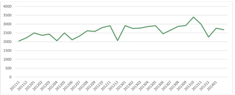
Figure 3.1: Historical data for ABB time series for the period 201111- 201402

201111 201112 201201 201202 201203 201204 201205 201206 201207 201208 201209 201210 201211 201212 2043 2225 2501 2366 2431 2056 2499 2111 2327 2620 2585 2805 2905 2066 201301 201302 201303 201304 201305 201306 201307 201308 201309 201310 201311 201312 201401 201402

2911 2755 2772 2861 2908 2452 2661 2871 2922 3395 2998 2269 2765 2681 Table 3.2: Historical data for BB_ABB time series for the period 201111-201402

Looking at the data for the number of cases in this degree project, we accept that it’s difficult to predict. We can’t define all the factors behind the case numbers for BB “Barnbidrag” and GP “Graviditetspenning”. Also looking at the prediction error correlation for the BB_ABB and GP_ANS in Figures 3.3, 3.7, and 3.13, we see that it has no sufficient values for all lags. That is also another indicator that the time series are difficult to predict. 0 500 1000 1500 2000 2500 3000 3500 4000

(19)

Horizon (Months) MAPE

(Mean Absolute Percentage Error) Observations Average Forecast Error

1 11,00% 24 2,40% 2 11,50% 24 -1,30% 3 10,90% 23 4,20% 4 16,80% 23 3,00% 5 15,20% 22 3,60% 6 14,70% 22 6,20% 7 18,30% 22 5,70% 8 17,40% 21 5,70% 9 17,90% 21 9,40% 10 21,40% 21 7,50% 11 21,10% 20 10,10% 12 18,90% 20 10,60% 13 19,00% 20 11,30% 14 24,70% 20 4,60% 15 17,50% 15 12,10% 16 23,30% 15 7,60% 17 20,20% 10 10,30% 18 16,40% 10 15,80% 19 26,90% 10 9,10% 20 18,90% 5 9,10% 21 17,90% 5 13,60% 22 31,40% 5 -0,90% Mean of total 18,70% 7,30%

Table 3.3: Absolute values of BB_ABB Forecast errors divided on different horizons.

3.1.2 Assumptions and Method Description

The number of cases will increase since the number of children is increasing in Sweden due to population growth. According to Statistics Sweden Agency (SCB), the population will continue to grow. That means we can assume that the BB_ABB time series has an upward trend.

AP uses time series models for forecasting in the short term. In the long term, the forecasts for ABB are based on SCB’s forecast for children aged 0-16. Data collection, parameter estimation, Autocorrelation Function (ACF), Partial Autocorrelation Function (PACF) calculations, and other computations are made using SAS. We can see in Figures 3.4 and 3.8 the forecasting view for BB_ABB cases starting from March 2014, and model and series viewing in Figures 3.2-3.13. Several different models have been tested using SAS.

(20)

3.1.3 Parameter Estimation

We will use a Seasonal Exponential Smoothing model of the form (10)-(13). The parameters of the model as estimated by SAS are given in the table below.

Component Parameter Estimate Standard Error

BB_ABB Level Weight 0,07729 0,05171

BB_ABB Trend Weight 0,001 0,01973

BB_ABB Seasonal Weight 0,001 0,13085 Where:

Level weight is α Smoothing constant for level Trend weight is γ Smoothing constant for trend

Seasonal weight is δ Smoothing constant for seasonal factor.

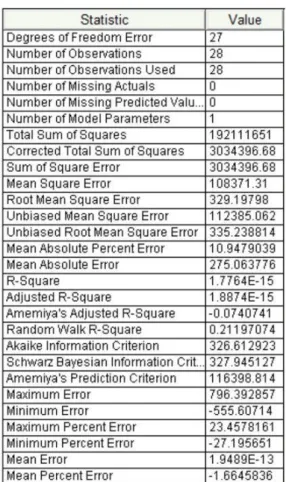
We will use an ARIMA (0,0,0) model of the form (3). The parameters of the model as estimated by SAS are given in the table below,

BB_ABB Constant 2598,6 63,35418

Where:

Estimate is the mean μ

Standard error is the standard error of the estimate of μ

(The standard deviation of the data can be found in the appendix Table1.)

There can be several methods to estimate the parameter in ARIMA models. For example, The generalized method of moments (GMM), maximum likelihood, and least squares. Those methods can be used to

estimate the parameters in the primarily identified model. Most of ARIMA models are nonlinear and require the use of a nonlinear model fitting procedure. This is automatically performed by SAS. In other software packages, the user can choose the estimation method and choose accordingly the most appropriate method based on the problem specification.

In order to get good forecasting using (ARIMA) models, we should have at least 50 observations, but preferably more than 100 observations [13]. The primary driving force behind these numbers is that if there are seasonal components, we'll need several years’ worth of monthly observations to appropriately model that out. However due to frequent changes to regulations and workflows, it is rare to have so many observations without changes to the underlying theoretical data generating function.

The parameter estimation is done by the SAS software for both models, and we will not discuss the procedure here in further detail. You may find the codes in the appendix.

(21)

3.1.4 Modeling view for ARIMA BB_ABB

Figure 3.2: Prediction Error White Noise Probability (Log Scale)

Figure 3.3: Prediction Error Correlation

Figure 3.4: Model and Forecasts

(22)

3.1.5 Modeling view for SES BB_ABB

(23)

3.1.6 Series view for BB_ABB

Figure 3.10: White Noise probabilities

Figure 3.11: Seasonal Decomposition/Adjustment

(24)

3.2 Pregnancy benefit

Pregnancy benefit (Graviditetspenning in Swedish or “GP”) is money that you can get if you have a physically demanding job or there are risks in your working environment that mean that you cannot work when you are pregnant.

We will only consider GP_ANS (Application for Pregnancy benefit). FK received more than 27 700 cases in the year 2019, and we can see March 2020 forecast in Table 3.4 as an example of forecasting.

2019¹ 2020² 2021² 2022² 2023²

GP_ANS 27 713 27 917 28 404 28 783 29 066

¹ Result Table 3.4: March 2020 forecast for Pregnancy benefit case volumes in 2020-2023

² Forecast

3.2.1 Forecast for case volumes within pregnancy benefit

The dataset for GP_ANS in this degree project starts from February 2012 with a continuous monthly result until February 2014, the forecasting starts from March 2014.

The numbers of cases between February 2012 and February 2014 are shown in Figure 3.14 and Table 3.5. The Absolute values of GP_ANS Forecast errors divided on different horizons can be found in Table 3.6.

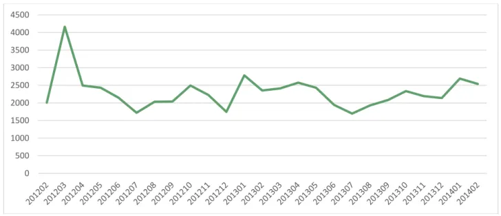
Figure 3.14: Historical data for GP_ANS time series for the period 201111-201402

201202 201203 201204 201205 201206 201207 201208 201209 201210 201211 201212 201301 201302 2011 4163 2495 2433 2147 1720 2033 2043 2495 2224 1745 2784 2355 201303 201304 201305 201306 201307 201308 201309 201310 201311 201312 201401 201402

2415 2577 2432 1942 1698 1930 2083 2336 2194 2138 2692 2540 Table 3.5: Historical data for GP_ANS time series for the period 201202-201402 0 500 1000 1500 2000 2500 3000 3500 4000 4500

(25)

Horizon (Months)

MAPE

(Mean Absolute Percentage Error) Observations Average Forecast Error

1 4,80% 24 -3,50% 2 5,70% 24 -3,60% 3 4,50% 23 -1,00% 4 5,30% 23 -3,20% 5 5,00% 22 -3,00% 6 5,20% 22 -2,80% 7 6,30% 22 -3,80% 8 5,90% 21 -3,10% 9 5,60% 21 -3,50% 10 5,90% 21 -4,30% 11 5,70% 20 -4,40% 12 4,20% 20 -3,00% 13 6,90% 20 -6,20% 14 7,90% 20 -7,20% 15 4,50% 15 -3,60% 16 8,50% 15 -7,00% 17 7,10% 10 -6,90% 18 4,40% 10 -3,70% 19 9,80% 10 -8,60% 20 7,00% 5 -7,00% 21 5,70% 5 -5,70% 22 12,80% 5 -11,30% Mean of total 6,30% -4,80%

Table 3.6: Absolute values of GP_ANS Forecast errors divided on different horizons 3.2.2 Assumptions and Method Description

The number of cases will increase as the number of born children is increasing in Sweden as per Statistics Sweden Agency (SCB) population projection. That means we can assume that GP_ANS time series has an upward trend.

The forecast for the number of application cases in pregnancy allowance is calculated using a time series model of measure GP_ANS. The time series model is used for short term forecasting. For the remainder of the forecast period, the same rate of change is assumed as for the number of births in the population forecast from Statistics Sweden (SCB). I will use SAS as well for collecting data, estimating parameters, calculating ACF and PACF, and other computations (Figures 3.15-3.26). Several models had been tested with SAS.

(26)

3.2.3 Parameter Estimation

We will use a Seasonal Exponential Smoothing model of the form (10)-(13). The parameters of the model as estimated by SAS are given in the table below.

GP_ANS Level Weight 0,06564 0,04764

GP_ANS Trend Weight 0,001 0,036

GP_ANS Seasonal Weight 0,001 0,17118

Where:

Level weight is α Smoothing constant for level Trend weight is γ Smoothing constant for trend

Seasonal weight is δ Smoothing constant for seasonal factor.

We will use an ARIMA (0,1,1) (0,1,0) model without an intercept (the mu parameter set to zero) of the form (7). The parameters of the model as estimated by SAS are given in the table below,

GP_ANS MA1_1 0,83950 0,16314

Where:

Estimate is

θ

the moving average parameter.

Standard error is the standard error of the estimate of

θ

(The standard deviation of the data can be found in the appendix Table 2.)

Most of ARIMA models are nonlinear and require the use of a nonlinear model fitting procedure. This is automatically performed by SAS. In other software packages, the user can choose the estimation method and choose accordingly the most appropriate method based on the problem specification.

The parameter estimation is done by the SAS software for both models, and we will not discuss the procedure here in further detail. You may find the codes in the appendix.

(27)

3.2.4 Modeling view for ARIMA GP_ANS

(28)

3.2.5 Modeling view for SES GP_ANS

(29)

2.2.6 Series view for GP_ANS

Figure 3.23: White Noise probabilities

Figure 3.24: Seasonal Decomposition/Adjustment

Figure 3.25: Series Values

(30)

4 Results

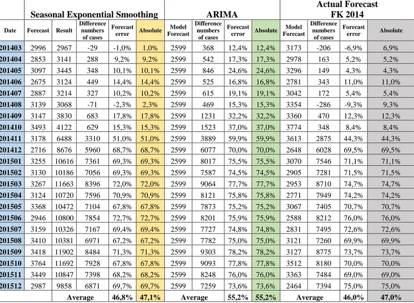
In the below Tables 4.1-4.4 and Figures 4.1-4.8, we can see a comparison of the forecast errors of each of those three models in the short and long term. That can give us a better understanding of the suggested models performed better on different horizons.

Seasonal Exponential Smoothing ARIMA

Actual Forecast FK 2014

Date Forecast Result

Difference numbers of cases Forecast error Absolute Model Forecast Difference numbers of cases Forecast error Absolute Model Forecast Difference numbers of cases Forecast error Absolute 201403 2996 2967 -29 -1,0% 1,0% 2599 368 12,4% 12,4% 3173 -206 -6,9% 6,9% 201404 2853 3141 288 9,2% 9,2% 2599 542 17,3% 17,3% 2978 163 5,2% 5,2% 201405 3097 3445 348 10,1% 10,1% 2599 846 24,6% 24,6% 3296 149 4,3% 4,3% 201406 2675 3124 449 14,4% 14,4% 2599 525 16,8% 16,8% 2781 343 11,0% 11,0% 201407 2887 3214 327 10,2% 10,2% 2599 615 19,1% 19,1% 3042 172 5,4% 5,4% 201408 3139 3068 -71 -2,3% 2,3% 2599 469 15,3% 15,3% 3354 -286 -9,3% 9,3% 201409 3147 3830 683 17,8% 17,8% 2599 1231 32,2% 32,2% 3360 470 12,3% 12,3% 201410 3493 4122 629 15,3% 15,3% 2599 1523 37,0% 37,0% 3774 348 8,4% 8,4% 201411 3178 6488 3310 51,0% 51,0% 2599 3889 59,9% 59,9% 3613 2875 44,3% 44,3% 201412 2716 8676 5960 68,7% 68,7% 2599 6077 70,0% 70,0% 2648 6028 69,5% 69,5% 201501 3255 10616 7361 69,3% 69,3% 2599 8017 75,5% 75,5% 3070 7546 71,1% 71,1% 201502 3130 10186 7056 69,3% 69,3% 2599 7587 74,5% 74,5% 2905 7281 71,5% 71,5% 201503 3267 11663 8396 72,0% 72,0% 2599 9064 77,7% 77,7% 2953 8710 74,7% 74,7% 201504 3124 10720 7596 70,9% 70,9% 2599 8121 75,8% 75,8% 2771 7949 74,2% 74,2% 201505 3368 10472 7104 67,8% 67,8% 2599 7873 75,2% 75,2% 3067 7405 70,7% 70,7% 201506 2946 10800 7854 72,7% 72,7% 2599 8201 75,9% 75,9% 2588 8212 76,0% 76,0% 201507 3159 10326 7167 69,4% 69,4% 2599 7727 74,8% 74,8% 2831 7495 72,6% 72,6% 201508 3410 10381 6971 67,2% 67,2% 2599 7782 75,0% 75,0% 3121 7260 69,9% 69,9% 201509 3418 11902 8484 71,3% 71,3% 2599 9303 78,2% 78,2% 3127 8775 73,7% 73,7% 201510 3764 11692 7928 67,8% 67,8% 2599 9093 77,8% 77,8% 3512 8180 70,0% 70,0% 201511 3449 10847 7398 68,2% 68,2% 2599 8248 76,0% 76,0% 3363 7484 69,0% 69,0% 201512 2987 9858 6871 69,7% 69,7% 2599 7259 73,6% 73,6% 2464 7394 75,0% 75,0%

Average 46,8% 47,1% Average 55,2% 55,2% Average 46,0% 47,0%

Table 4.1: Comparison of BB_ABB Forecast errors for the three models on the short term

Difference numbers of cases Forecast error Absolute Model Forecast Difference numbers of cases Forecast error Absolute 201601 3526 9703 6177 63,7% 63,7% 2599 7104 73,2% 73,2% 201602 3401 10615 7214 68,0% 68,0% 2599 8016 75,5% 75,5% 201603 3538 10762 7224 67,1% 67,1% 2599 8163 75,9% 75,9% 201604 3395 10917 7522 68,9% 68,9% 2599 8318 76,2% 76,2% 201605 3640 10694 7054 66,0% 66,0% 2599 8095 75,7% 75,7% 201606 3217 10047 6830 68,0% 68,0% 2599 7448 74,1% 74,1% 201607 3430 9269 5839 63,0% 63,0% 2599 6670 72,0% 72,0% 201608 3681 11277 7596 67,4% 67,4% 2599 8678 77,0% 77,0% 201609 3689 13149 9460 71,9% 71,9% 2599 10550 80,2% 80,2% 201610 4035 12006 7971 66,4% 66,4% 2599 9407 78,4% 78,4% 201611 3720 12076 8356 69,2% 69,2% 2599 9477 78,5% 78,5% 201612 3258 10717 7459 69,6% 69,6% 2599 8118 75,8% 75,8%

(31)

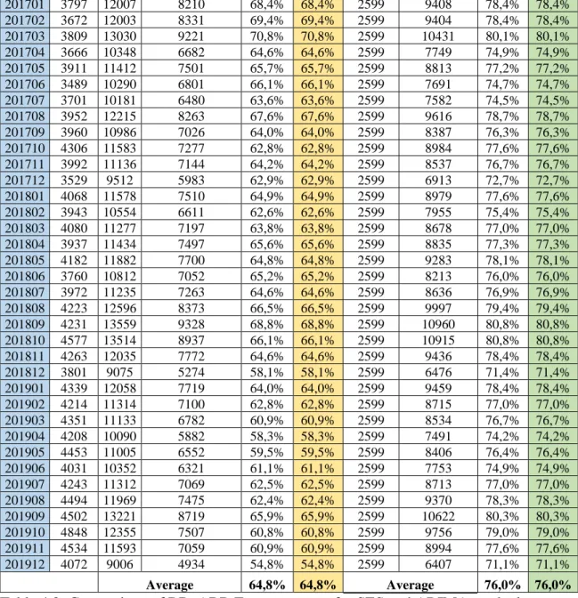
201701 3797 12007 8210 68,4% 68,4% 2599 9408 78,4% 78,4% 201702 3672 12003 8331 69,4% 69,4% 2599 9404 78,4% 78,4% 201703 3809 13030 9221 70,8% 70,8% 2599 10431 80,1% 80,1% 201704 3666 10348 6682 64,6% 64,6% 2599 7749 74,9% 74,9% 201705 3911 11412 7501 65,7% 65,7% 2599 8813 77,2% 77,2% 201706 3489 10290 6801 66,1% 66,1% 2599 7691 74,7% 74,7% 201707 3701 10181 6480 63,6% 63,6% 2599 7582 74,5% 74,5% 201708 3952 12215 8263 67,6% 67,6% 2599 9616 78,7% 78,7% 201709 3960 10986 7026 64,0% 64,0% 2599 8387 76,3% 76,3% 201710 4306 11583 7277 62,8% 62,8% 2599 8984 77,6% 77,6% 201711 3992 11136 7144 64,2% 64,2% 2599 8537 76,7% 76,7% 201712 3529 9512 5983 62,9% 62,9% 2599 6913 72,7% 72,7% 201801 4068 11578 7510 64,9% 64,9% 2599 8979 77,6% 77,6% 201802 3943 10554 6611 62,6% 62,6% 2599 7955 75,4% 75,4% 201803 4080 11277 7197 63,8% 63,8% 2599 8678 77,0% 77,0% 201804 3937 11434 7497 65,6% 65,6% 2599 8835 77,3% 77,3% 201805 4182 11882 7700 64,8% 64,8% 2599 9283 78,1% 78,1% 201806 3760 10812 7052 65,2% 65,2% 2599 8213 76,0% 76,0% 201807 3972 11235 7263 64,6% 64,6% 2599 8636 76,9% 76,9% 201808 4223 12596 8373 66,5% 66,5% 2599 9997 79,4% 79,4% 201809 4231 13559 9328 68,8% 68,8% 2599 10960 80,8% 80,8% 201810 4577 13514 8937 66,1% 66,1% 2599 10915 80,8% 80,8% 201811 4263 12035 7772 64,6% 64,6% 2599 9436 78,4% 78,4% 201812 3801 9075 5274 58,1% 58,1% 2599 6476 71,4% 71,4% 201901 4339 12058 7719 64,0% 64,0% 2599 9459 78,4% 78,4% 201902 4214 11314 7100 62,8% 62,8% 2599 8715 77,0% 77,0% 201903 4351 11133 6782 60,9% 60,9% 2599 8534 76,7% 76,7% 201904 4208 10090 5882 58,3% 58,3% 2599 7491 74,2% 74,2% 201905 4453 11005 6552 59,5% 59,5% 2599 8406 76,4% 76,4% 201906 4031 10352 6321 61,1% 61,1% 2599 7753 74,9% 74,9% 201907 4243 11312 7069 62,5% 62,5% 2599 8713 77,0% 77,0% 201908 4494 11969 7475 62,4% 62,4% 2599 9370 78,3% 78,3% 201909 4502 13221 8719 65,9% 65,9% 2599 10622 80,3% 80,3% 201910 4848 12355 7507 60,8% 60,8% 2599 9756 79,0% 79,0% 201911 4534 11593 7059 60,9% 60,9% 2599 8994 77,6% 77,6% 201912 4072 9006 4934 54,8% 54,8% 2599 6407 71,1% 71,1% Average 64,8% 64,8% Average 76,0% 76,0%

Table 4.2: Comparison of BB_ABB Forecast errors for SES and ARIMA on the long term

(32)

Figure 4.2: BB_ABB Absolute forecast errors for ARIMA model for the period 201402-201911

Figure 4.3: BB_ABB Absolute forecast errors for the actual forecast for the period 201402-201911

Figure 4.4: Comparison of BB_ABB forecast errors for the three models 0,0% 10,0% 20,0% 30,0% 40,0% 50,0% 60,0% 70,0% 80,0%

(33)

Actual Forecast FK 2014

Difference numbers of cases Forecast error Absolute Model Forecast Difference numbers of cases Forecast error Absolute Model Forecast Difference numbers of cases Forecast error Absolute 201403 3231 2607 -624 -23,9% 23,9% 2452 155 5,9% 5,9% 2850 -243 -9,3% 9,3% 201404 2478 2485 7 0,3% 0,3% 2614 -129 -5,2% 5,2% 2491 -6 -0,2% 0,2% 201405 2375 2442 67 2,7% 2,7% 2469 -27 -1,1% 1,1% 2463 -21 -0,9% 0,9% 201406 1987 2233 246 11,0% 11,0% 1979 254 11,4% 11,4% 2255 -22 -1,0% 1,0% 201407 1652 1755 103 5,9% 5,9% 1735 20 1,1% 1,1% 1700 55 3,1% 3,1% 201408 1925 1935 10 0,5% 0,5% 1967 -32 -1,7% 1,7% 2041 -106 -5,5% 5,5% 201409 2006 2310 304 13,2% 13,2% 2120 190 8,2% 8,2% 2380 -70 -3,0% 3,0% 201410 2359 2568 209 8,1% 8,1% 2373 195 7,6% 7,6% 2352 216 8,4% 8,4% 201411 2153 2093 -60 -2,8% 2,8% 2231 -138 -6,6% 6,6% 2366 -273 -13,0% 13,0% 201412 1885 2048 163 7,9% 7,9% 2175 -127 -6,2% 6,2% 2204 -156 -7,6% 7,6% 201501 2682 2607 -75 -2,9% 2,9% 2729 -122 -4,7% 4,7% 2703 -96 -3,7% 3,7% 201502 2220 2462 242 9,8% 9,8% 2577 -115 -4,7% 4,7% 2604 -142 -5,8% 5,8% 201503 3181 2653 -528 -19,9% 19,9% 2490 163 6,2% 6,2% 3029 -376 -14,2% 14,2% 201504 2428 2549 121 4,7% 4,7% 2652 -103 -4,0% 4,0% 2648 -99 -3,9% 3,9% 201505 2325 2366 41 1,7% 1,7% 2507 -141 -6,0% 6,0% 2617 -251 -10,6% 10,6% 201506 1937 2454 517 21,1% 21,1% 2017 437 17,8% 17,8% 2397 57 2,3% 2,3% 201507 1602 1777 175 9,9% 9,9% 1773 4 0,2% 0,2% 1807 -30 -1,7% 1,7% 201508 1874 2038 164 8,0% 8,0% 2005 33 1,6% 1,6% 2170 -132 -6,5% 6,5% 201509 1956 2476 520 21,0% 21,0% 2158 318 12,8% 12,8% 2529 -53 -2,1% 2,1% 201510 2309 2466 157 6,4% 6,4% 2411 55 2,2% 2,2% 2499 -33 -1,3% 1,3% 201511 2102 2454 352 14,3% 14,3% 2269 185 7,5% 7,5% 2514 -60 -2,4% 2,4% 201512 1835 2436 601 24,7% 24,7% 2213 223 9,2% 9,2% 2342 94 3,9% 3,9%

Average 5,5% 10,0% Average 2,3% 6,0% Average -3,4% 5,0%

Table 4.3: Comparison of GP_ANS Forecast errors for the three models on the short term

Date Forecast Result

Difference numbers of cases Forecast error Absolute Model Forecast Difference numbers of cases Forecast error Absolute 201601 2632 2682 50 1,9% 1,9% 2767 -85 -3,2% 3,2% 201602 2169 2584 415 16,0% 16,0% 2615 -31 -1,2% 1,2% 201603 3131 2602 -529 -20,3% 20,3% 2527 75 2,9% 2,9% 201604 2378 2723 345 12,7% 12,7% 2689 34 1,2% 1,2% 201605 2275 2632 357 13,6% 13,6% 2544 88 3,3% 3,3% 201606 1887 2305 418 18,1% 18,1% 2054 251 10,9% 10,9% 201607 1551 1649 98 5,9% 5,9% 1810 -161 -9,8% 9,8% 201608 1824 2125 301 14,2% 14,2% 2042 83 3,9% 3,9% 201609 1906 2445 539 22,1% 22,1% 2553 -108 -4,4% 4,4% 201610 2258 2461 203 8,2% 8,2% 2543 -82 -3,3% 3,3% 201611 2052 2431 379 15,6% 15,6% 2450 -19 -0,8% 0,8% 201612 1785 2149 364 16,9% 16,9% 2430 -281 -13,1% 13,1% 201701 2581 2711 130 4,8% 4,8% 2804 -93 -3,4% 3,4% 201702 2119 2385 266 11,1% 11,1% 2652 -267 -11,2% 11,2% 201703 3080 2785 -295 -10,6% 10,6% 2565 220 7,9% 7,9% 201704 2328 2322 -6 -0,2% 0,2% 2727 -405 -17,4% 17,4% 201705 2224 2674 450 16,8% 16,8% 2582 92 3,5% 3,5% 201706 1837 2250 413 18,4% 18,4% 2092 158 7,0% 7,0% 201707 1501 1777 276 15,5% 15,5% 1848 -71 -4,0% 4,0%

(34)

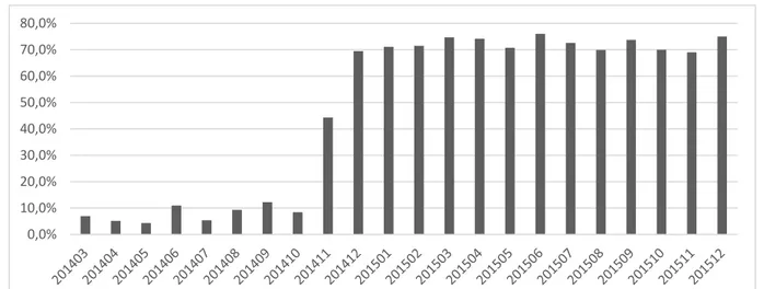
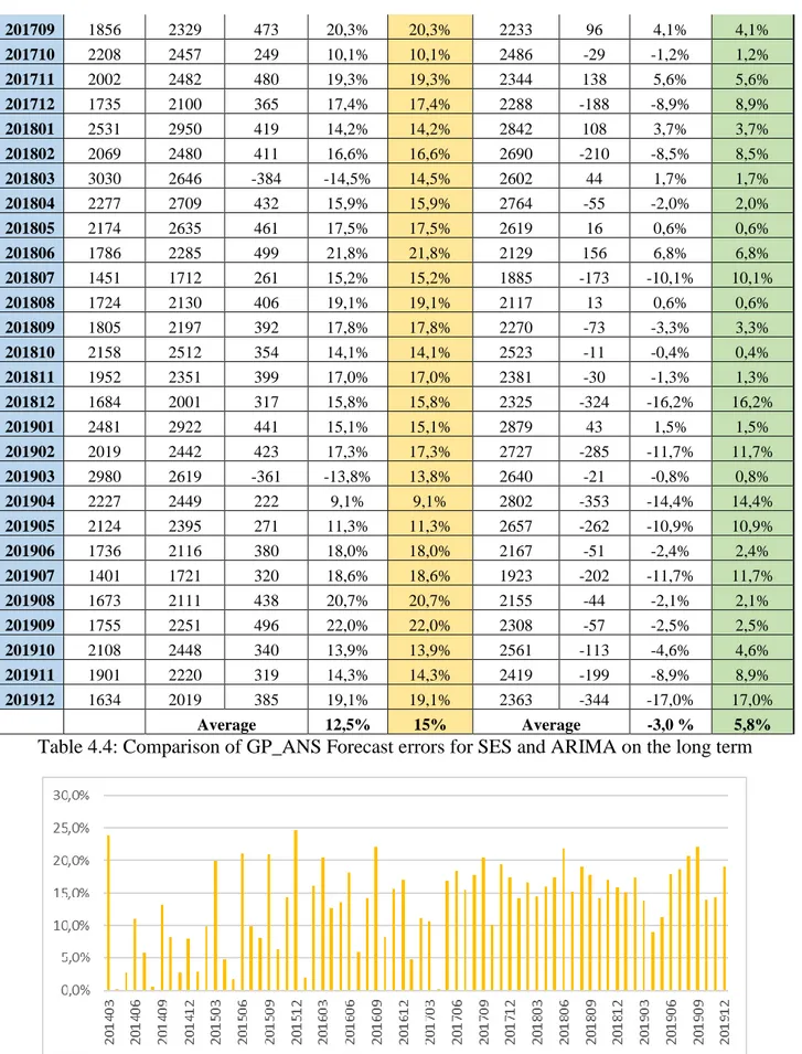
201709 1856 2329 473 20,3% 20,3% 2233 96 4,1% 4,1% 201710 2208 2457 249 10,1% 10,1% 2486 -29 -1,2% 1,2% 201711 2002 2482 480 19,3% 19,3% 2344 138 5,6% 5,6% 201712 1735 2100 365 17,4% 17,4% 2288 -188 -8,9% 8,9% 201801 2531 2950 419 14,2% 14,2% 2842 108 3,7% 3,7% 201802 2069 2480 411 16,6% 16,6% 2690 -210 -8,5% 8,5% 201803 3030 2646 -384 -14,5% 14,5% 2602 44 1,7% 1,7% 201804 2277 2709 432 15,9% 15,9% 2764 -55 -2,0% 2,0% 201805 2174 2635 461 17,5% 17,5% 2619 16 0,6% 0,6% 201806 1786 2285 499 21,8% 21,8% 2129 156 6,8% 6,8% 201807 1451 1712 261 15,2% 15,2% 1885 -173 -10,1% 10,1% 201808 1724 2130 406 19,1% 19,1% 2117 13 0,6% 0,6% 201809 1805 2197 392 17,8% 17,8% 2270 -73 -3,3% 3,3% 201810 2158 2512 354 14,1% 14,1% 2523 -11 -0,4% 0,4% 201811 1952 2351 399 17,0% 17,0% 2381 -30 -1,3% 1,3% 201812 1684 2001 317 15,8% 15,8% 2325 -324 -16,2% 16,2% 201901 2481 2922 441 15,1% 15,1% 2879 43 1,5% 1,5% 201902 2019 2442 423 17,3% 17,3% 2727 -285 -11,7% 11,7% 201903 2980 2619 -361 -13,8% 13,8% 2640 -21 -0,8% 0,8% 201904 2227 2449 222 9,1% 9,1% 2802 -353 -14,4% 14,4% 201905 2124 2395 271 11,3% 11,3% 2657 -262 -10,9% 10,9% 201906 1736 2116 380 18,0% 18,0% 2167 -51 -2,4% 2,4% 201907 1401 1721 320 18,6% 18,6% 1923 -202 -11,7% 11,7% 201908 1673 2111 438 20,7% 20,7% 2155 -44 -2,1% 2,1% 201909 1755 2251 496 22,0% 22,0% 2308 -57 -2,5% 2,5% 201910 2108 2448 340 13,9% 13,9% 2561 -113 -4,6% 4,6% 201911 1901 2220 319 14,3% 14,3% 2419 -199 -8,9% 8,9% 201912 1634 2019 385 19,1% 19,1% 2363 -344 -17,0% 17,0% Average 12,5% 15% Average -3,0 % 5,8%

Table 4.4: Comparison of GP_ANS Forecast errors for SES and ARIMA on the long term

(35)

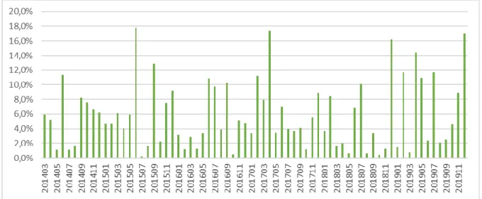
Figure 4.6: GP_ANS Absolut forecast errors for ARIMA model for the period 201402-201911

Figure 4.7: GP_ANS Absolut forecast errors for the actual forecast for the period 201402-201911

Figure 4.8: Comparison of GP_ANS Forecast errors for the three models 0,0% 2,0% 4,0% 6,0% 8,0% 10,0% 12,0% 14,0% 16,0%

(36)

5 Conclusion

We examine two measures of forecast errors, which are absolute error and forecast error. The forecasting model ARIMA for GP_ANS has forecast errors on the short and long horizons, which were lower than the forecasting model used by FK in March 2014. However, the absolute error is lower in the used model. It is shown in Tables 4.3 and 4.4 as well as Figures 4.5-4.8. The difference between these error measures is important for the planning of the needed recourse. As the absolute error will not show if there are more or fewer resources required. For example, a positive forecast error means that the actual number of cases is higher than the forecasted number, which would require more resources to confirm.

It also shows that using time series forecasting in the long term sometimes yields better results than building it on an external rate of change (e.g. SCB). Furthermore, it requires less quarterly manual adjustment by the forecaster.

However, it also shows that in some cases, long-term forecasting can have a much larger forecast error if the forecaster does not adjust it manually on a quarterly basis as a law or rules change. In addition, external changes in the societal circumstances can produce high forecast error. For example, BB_ABB has large forecast errors in the long term due to rules changes, new classifications, and the refugee crisis in 2015. All of these circumstances combined increased the number of BB_ABB cases dramatically. The forecast errors for the different models shown in Tables 4.1 and 4.2 as well as Figures 4.1-4.4.

As we mentioned previously, in order to get good forecasting using (ARIMA) models, we should have at least 50 observations but preferably more than 100 observations. We got a constant number for BB_ABB because the ARIMA (0,1,0) process predicts that on average the value should stay the same, and this mean is the parameter that is estimated by SAS.

Therefore, this means that it is probably not feasible to do forecasting of those time series with all the tested models in the long-term. However, that mainly depends on what FK considers as accepted forecast errors and how those forecasts will be used.

6 Further work

For further research, it would be interesting to compare other social insurance benefits with the same models. It would also be interesting to test BB_ABB and GP_ANS in different time periods to see how the models will perform. As only 2 social benefit cases were covered in this degree project, further work can be done where more examples are explored and the influence of the noise is examined. Another extension can be examining the stability and noise sensitivity of the models, and finding a way to use more observations by covering other periods, this could lead to making ARIMA models more certain. If we want to use data for longer periods, we also need to find a way to compensate for the changes in laws and rules and external changes in circumstances.

(37)

7 Summary of the reflection of the objectives in the thesis

A summary of the objectives accomplished in this thesis will be presented in this chapter.

7.1 Objective 1: Knowledge and Understanding

I researched many journal articles and books related to time series analysis and forecasting during the process of writing this thesis. I investigated various methods that FK uses for forecasting. I decided that the used methods were the best choice for my thesis for the reasons mentioned in the thesis. I had difficulty in finding research material related to the forecast made in 2014 as the majority of the material available was on later dates. Hence, I used designs that would normally be used if no information about the data sets or models were provided. I did explore real-life examples, and I believe that the applications of the designs would work similarly to other real-life examples.

7.2 Objective 2: Methodological Knowledge

I approached the concept by first identifying what benefits cases and models were available in FK’s database. Next, I experimented with many types and models. Finally, I selected and compared the most popular forecasting models with the best-perfumed results.

7.3 Objective 3: Critically and Systematically Integrate Knowledge

The references used in this thesis were mainly books found through the MDH library portal and Google search. I also used the FK website and SAS guide books as references. The procedure of my thesis was broken up into three stages: literature review, experimentation, and write-up. I first studied literature

material on or related to time series analysis and forecasting. I then experimented with other models on SAS and tried to understand the results of the experiments. Finally, I started writing when I understood the comparisons of the models.

7.4 Objective 4: Independently and Creatively Identify and Carry out Advanced Tasks

In Chapter 3, I came up with the models based on what I picked up through the references which were a number of models that are commonly used by researchers. I did the SAS work in this thesis using the codes that FK provided me. I made similar codes and tested my models with them. I discussed my results with my supervisor and came up with the conclusions.

7.5 Objective 5: Present and Discuss Conclusions and Knowledge

A reader with moderate knowledge in applied mathematics will be able to understand the content of this thesis. The reader will need to have some understanding of time series analysis and forecast.

In the theory, I have presented the selected models for forecasting and also defined a

few terms that are used in the thesis. I have provided figures and tables to make it easier for the reader to understand the comparisons. I have also defined any new terms that may be unfamiliar

to a reader throughout the thesis. In the future work under Conclusions, I have put forward some extensions that can be done to this thesis.

7.6 Objective 7: Scientific, Social and Ethical Aspects

Online meetings were scheduled with my immediate supervisor Karl Lundengård and the manager of the forecasting department at FK (due to Coronavirus), based on the amount of work that could be completed. My supervisor regularly provided feedback via email after each update of the thesis was done.

(38)

8 Bibliography

[1] The Swedish Social Insurance budget and forecast, 2020-06

https://www.forsakringskassan.se/statistik/publikationer/budget-och-prognos

[2] Yule, G. U. (1927). "On a Method of Investigating Periodicities in Disturbed Series, with Special

Reference to Wolfer's Sunspot Numbers". Philosophical Transactions of the Royal Society A: Mathematical, Physical and Engineering Sciences. 226 (636–646): 267–298

[3] G. E. P. Box, G. M. Jenkins and G.C Reinsel , 1970. Time Series Analysis: Forecasting and Control. [4] Brown, Robert G. (1956). Exponential Smoothing for Predicting Demand. Cambridge, Massachusetts: Arthur D. Little Inc. p. 15.

[5] S. A. Roberts Management Science, Vol. 28, No. 7 (Jul., 1982), pp. 808-820.A General Class of Holt-Winters Type Forecasting Models

[6] Rob J Hyndman , George Athanasopoulos :Forecasting: principles and practice Paperback – October 17, 2013

[7] Chatfield, C. and Yar, M. (1988) Holt-Winters Forecasting: Some Practical Issues. Journal of the Royal Statistical Society. Series D (The Statistician), 37, 129-140.

[8] Douglas C. Montgomery, Cheryl L. Jennings, Murat Kulahci: Introduction to Time Series Analysis and Forecasting: – 2008

[9] Gardner, E. S., Jr. (1985). Exponential smoothing: The state of the art. Journal of Forecasting 4, 1–28 [10] Chatfield, C. (1978) The Holt-Winters Forecasting Procedure. Applied Statistics Chatfield, C. (1978) The Holt-Winters Forecasting Procedure. Applied Statistics, 27, 264-279.

[11] Bruce L. Bowerman, Richard T. O'Connell, 1979.Time Series and Forecasting: An Applied Approach. [12] Forecasting Process Details, SAS 9.3 User's Guide. 2020-05

https://support.sas.com/documentation/cdl/en/etsug/63939/HTML/default/viewer.htm#tffordet_toc.htm [13] Box, G. E. P., and G. C. Tiao. 1975. Intervention analysis with applications to economic and environmental problems. Journal of the American Statistical Association 70: 70(79).

[14] G. M. Ljung; G. E. P. Box (1978). "On a Measure of a Lack of Fit in Time Series Models". Biometrika. 65 (2): 297–303.

(39)

Appendix

Description of the used model on SAS forecasting for BB_ABB: ARIMA MAPE 12, 62 Name: ARIMA 1

Details: "ARIMA: Y ~ CONST" Model family: ARIMA

Model type: ARIMA

Source: FSU Intercept: Yes Forecast variable: Y Delay: 0 Differencing: ( 0 ) Estimation Options Method: CLS Convergence criterion: 0.001 Number of iterations: 50 Delta: 0.001

Singularity criterion: 1E-7 Grid value: 0.005

Restrict parameters to stable values: Yes NOLS: 0

Description of the used model on SAS forecasting for BB_ABB: SES MAPE 10,29 Details: "Seasonal Exponential Smoothing"

Model family: ESM Model type: ESM

Source: HPFDFL Model code: SEASONAL Selection code: RMSE

Transform: NONE Forecast option: MEAN Estimation options Component: LEVEL Lower: 0.001 Upper: 0.999 Component: TREND Lower: 0.001 Upper: 0.999 Component: SEASON Lower: 0.001 Upper: 0.999 Component: DAMPING Lower: 0.001 Upper: 0.999

Comparison of Forecasting Models Used by The Swedish Social Insurance Agency.

MASTER THESIS IN FINANCIAL ENGINEERING