Perishable Items in Multi-Level Inventory Systems

(1)

Perishable Items in Multi-Level Inventory Systems

Department of Industrial Management and Logistics, LTH

Master Thesis presented by Yann Bouchery

Double Degree Student

Ecole Centrale de Lille (France)

Lunds Tekniska Högskola (Sweden)

Supervisor: Fredrik Olsson

Assistant Professor

Department of Industrial Management and Logistics

Division of Production Management

Lund University, Faculty of Engineering LTH

Lund, June 2007

(2)

(3)

Abstract

This master thesis studies a two-echelon distribution system for perishable items with two non identical retailers. Each location is managed following a standard continuous (R, Q) ordering policy. The demand occurs solely at the retailers and follows independent Poisson processes. Customers are backordered when the retailer is out of stock. The items are considered as fixed lifetime perishables. Whenever an item perished, it is discarded from the stock. The model includes fix transportation time and the allocation policy at the central warehouse is a First-Come-First-Serve one.

This kind of system is very complicated and therefore hard to study. In this master thesis, we focus on a simulation study of 48 different problems with both a FIFO and a LIFO issuing policy at the retailers. The goal of this study is therefore to optimize the values of R in (R, Q) ordering policies considering that the items are perishables. To do so, we try to optimize the values of the reorder points at every location. We also try to find some general behaviour of the system and we compare the FIFO and the LIFO best found solution.

More than 1000 hours of computer-time were used for this study. For every problem, we conducted an optimization process to find better values of the reorder points at every location. For the FIFO case, an average cost reduction of more than 20% was found. It exists a good opportunity in term of cost savings while taking into account the perishable characteristic of the items. Another finding of our study is that the LIFO case has good performance comparing to what expected. On average, the costs increase is only 7% while considering a LIFO issuing policy instead of a FIFO one. Moreover, the values of the reorder points for the FIFO best found solution are still the same than the LIFO best found solution in 70% of the problems studied.

(4)

Foreword

This master thesis was made at the division of Production Management in the department of Industrial Management and Logistics at Lund Institute of Technology. This project is a starting point in the general study of the multi-echelon perishable inventory systems. Even if some particular cases are already studied, a lot has to be done in this field.

I would like to start by thanking my supervisor Fredrik Olsson, without his help and remarks, the making of this master thesis would not have been possible. I also would like to thank everyone working at the department for all the time and all the advices they gave me. They also helped me to feel welcome in Sweden as I lived in Lund for two years following the master program in industrial management and logistics. I would also thank you my home university, Ecole Centrale de Lille to allow me to follow this double degree program.

Last but not least, I thank my family and my girlfriend Delphine for supporting me during theses two nice years that I spent in Sweden.

(5)

Introduction

Inventory control is nowadays recognized as a crucial activity to succeed in a lot of businesses. The two main reasons explaining this fact are the need of a high service level and the low cost requirement to give customers the highest satisfaction. These two forces act unfortunately in opposite ways. On one hand, the uncertainty in the demand requires to keep enough stock to avoid shortage. One the other hand, the cost incurred by the capital tied up in inventories must be cut down by lowering inventory levels. As we will see later, the optimum solution is not easy to find even in very simple cases (see Chapter 1). When the situation becomes more complicated, it often does not exist any theoretical result to find the optimum. In this thesis, we focused on multi-echelon (or multi-level) inventory systems, where several stocks are linked somehow. This assumption makes the problem difficult to study as every modification in the inventory policy at one location has implications at every other location. Nevertheless, the field of stochastic multi-echelon inventory theory has a wide range of practical applications, as the majority of the supply chain systems can be modelled as multi-echelon systems.

The majority of the work in the inventory control theory assumes that there is no limit of the product’s storage time i.e. that the products keep all their usability whenever they are sold. In practice, this is obviously not the case for some products like provisions, photographic films, medicine or blood. From a theoretical point of view, every item will become unusable after a certain amount of time. From a practical point of view, only the products with short shelf life or product which will become unsaleable soon will be considered as perishables. For example, perishables stand for almost one third of the sales of the supermarket industry according to Broekmeulen and Van Donselaar (2007). The major characteristic of a perishable inventory system is that once the product lifetime is reached, the product must be discarded from the stock. In the supermarket industry, around 15% of the perishables are lost due to spoilage according to Lystad and Ferguson (2006). It is therefore important to study the perishable case to understand how to handle with perishable items into practice.

(7)

The goal of this master thesis is to study multi-echelon inventory systems for perishable items. We will describe the system chosen more into detail in the Chapter 4.It is important to notice that this kind of inventory system is very complicated to study. We therefore decided to focus on simulation to get some understanding about general behaviours of the system. Our main goal is to find good inventory policy for a range of problems and to evaluate if significant savings can be achieved by considering the items as perishable worth the work, both theoretical and practical, that has to be done to handle with this characteristic. Moreover, we will look for some trends and general behaviour of multi-echelon systems when considering the items as perishable. To understand better these systems, a starting point is to develop some approximate or some exact models to deal with perishable items in a multi-echelon environment.

This paper is written as followed. The introduction above describes briefly the subject of stochastic inventory theory and defines the goals of the study. Chapter 1 gives some background about inventory theory while Chapter 2 presents some important models related to our study both in the non perishable and in the perishable case. Chapter 3 includes the literature review carried out. Chapter 4 first presents the assumptions and constraints of the study and then describes the model chosen. Chapter 5 is dedicated to the methodology followed during this master thesis and Chapter 6 presents our results. Finally, the conclusion summarizes our main findings and gives suggestions for future researches.

(8)

1. Background: Inventory Control Theory

This section deals with some basics about inventory control from an academic point of view. The main goal of this section is to give the reader an insight about what kind of problems are already well studied and the methodology that is used to deal with this problem. In this section, we will use Axsäter (2006) as the main reference.

The first question that we have to answer is about the advantages and disadvantages to hold an inventory. Why holding stock?

As Axsäter (2006) points out, the two main reasons are uncertainties and economies of scale. The uncertainties are of different kind. The most important one is the demand uncertainty. In most of the real cases, the demand is not constant over the time and it is impossible to forecast it perfectly. Then there are also uncertainties about the order lead time and the estimation of the cost parameters. It can also be valuable to hold stock when economies of scale are possible by ordering a larger amount of items at one time.

Holding a larger stock is often the solution used by the firms to deal with the real supply chain problems. This is obviously not an appropriate solution, there are indeed a lot of reasons not to hold inventory.

Consequently, we have to find the balance between the advantages and drawbacks resulting from holding stock, to try to find the optimal stock policy.

There are a lot of parameters that have to be taken into account when dealing with an inventory problem. In this entire chapter, we will only consider single-item inventory systems. This assumption is not very restrictive, as it is often possible to control the different items independently, that is to say, to decompose your inventory into several single-item inventory systems.

In the next section, we will present one of the simplest cases of inventory problems, the single-item single-echelon inventory system.

(9)

1.1 Single echelon inventory systems

A single echelon inventory system is a supply chain system with only one location (one stock). Even if this model seems to be very restrictive, it is the most used in practice. The reason for that is the decentralization of the majority of the supply chain systems between different companies. We will see in the Section 1.2 that this decomposition of the supply chain into several single echelon inventory systems is far from optimal, however, the theoretical optimality is counterbalance by the difficulty to share information and the difficulty to trust the other companies enough. There is also a problem of cost repartition between the different actors.

There are series of questions arising when constructing an inventory model:

What type of reviewing policy do we want to implement? (Continuous vs. periodic review) Nowadays, with the expansion of the information technology, it is possible to review an inventory system continuously (review time = 0). However the periodic review is still the most used in practice (review time > 0).

What type of ordering policy do we want to implement? (R, Q), (s, S), other?

The ordering policy deals with the batch size ordered and the moment to place an order. In most of the cases with single-echelon systems, the (s, S) policy is proved to be optimal. Nevertheless, even in simple cases, the optimal ordering policy can be much more complicated. On the other hand, these complicated policies will not be implemented into practice as it will become too difficult to manage the stock. There are indeed two main ordering policies used.

(s, S) policy: In this inventory system, we will order up to S as soon as the inventory position (stock on hand + outstanding orders – backorders) declines to or below s. The order will arrive L time unit after ordered.

(R, Q) policy: This policy is quite similar to the (s, S) one, but in this case, the batch size ordered is constant equal to Q. We will order a batch of Q units as soon as the inventory position declines to or below R. Sometimes, in a periodic review case, it is necessary to order a multiple of Q batches to get the inventory position larger than R.

(10)

It is important to notice that in the continuous review and continuous demand case, an (s, S) policy is equivalent to a (R, Q) one, with s = R and S = R + Q.

What type of issuing policy will we used? (FIFO, LIFO)

The issuing policy plays a major role when items are perishables. The freshness of the product becomes a major matter for the customers who will try to buy the fresher product. The most common issuing policy is the First In First Out (FIFO) policy. For this policy, the first item arriving in the inventory will be sold first. However, the Last In First Out policy (LIFO) can be more close to practice when customer can choose the products (as in a supermarket). We will now present an example of calculation which is also the most well know inventory control problem. This problem is called the classical economic order quantity formula. Even if this is one of the simplest problems, its practical use is enormous. It was first derived by Harris (1913).

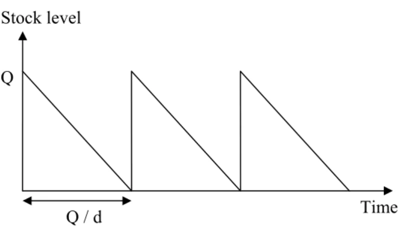
This problem is a single-echelon single-product problem with constant and continuous demand over the time (d: demand per time unit). The shortages are not allowed and the lead time is equal to zero. Moreover, the holding cost per unit and time unit is equal to h > 0 and the ordering cost is equal to A > 0 (per order). The ordering policy used is the (R, Q) type. First of all, since no shortage is allowed and as there is no need of safety stock (as the demand is deterministic), the optimal is found for R = 0. A batch of size Q is delivered exactly when the last unit in stock is consumed. Moreover, as the leadtime is equal to 0, this batch is ordered exactly when the last unit in stock in consumed. The inventory level will vary over the time as in the Figure 1:

Stock level

Time Q

Q / d

(11)

Consequently, the total cost formula can be formulated as: A Q d h Q C = × + × 2

The optimum is found by derivation of this formula, as C is convex in Q. This gives:

h d A Q* = 2× × and h d A C* = 2× × ×

A lot of different assumptions can be made to refine this example. We will not enter into details here. The main drawback of this model is certainly to consider the demand deterministic and constant over the time. But this model is still very important because a well known technique in inventory control is to approximate the probabilistic case by the deterministic case with the same average demand to determine the batch size Q. Then, the probabilistic case is studied to determine the value of reorder point R.

If the demand is still deterministic but non constant over the time, the problem is called the dynamic lot size problem. It exists exact and approximate methods to deal with this problem in the periodic review case. The Wagner-Within algorithm is an exact method based on dynamic programming while the Silver-Meal heuristic is an approximation much simpler to implement. In practice, it is much more common to use an approximation because these lot sizing technique are usually applied in a rolling horizon environment. In this case, if the time horizon is short, the Wagner-Within algorithm is also an approximation and it is more sensitive with respect to the time horizon than the approximation methods.

We will now study the case where the demand follows a probability distribution (non deterministic demand). In the probabilistic case, our main concern is to evaluate the optimal reorder point (this is a common approximation to use the deterministic case to evaluate the batch size). To do so, we have to derive the probabilities of the inventory level for every value of j, P (IL=j).

(12)

If we consider a continuous review (R, Q) policy system, allowing backorders (b = backorder cost per unit and time unit) and using the same notation than for the classical economic order quantity problem (d is now the average demand per time unit), the cost structure is now:

∑

⋅ −∞ = = + = ⋅ ⋅ − = ⋅ ⋅ + = 0 ) ( ) ( Q R k IL P k b k IL P k h d A C ₀ k k Q

We can choose to optimize both R and Q or only R (as we said before).

1.2 Multi-echelon inventory systems

An inventory system is considered to be multi-echelon (or multi-level) when several stocks are linked in a certain way. This is the case in most of the real supply chain systems, even if the single-echelon approximation is often used to simplify the problem. There are three different kind of multi-echelon inventory systems:

The serial system: Each inventory is supplied by one other location (in maximum) and supplies in its turn one other location (in maximum). These systems are very useful in theory as they are quite simple to study, but they are not so common in the reality.

The distribution system (divergent structure): Each inventory is supplied by one location (in maximum) and supplies in its turn a number of other locations (except from the more downstream inventories). A common example of a distribution system is the case where a central warehouse supplies several retailers. This example is called a two-echelon distribution system.

The production system (convergent structure): Each inventory is supplied by several other locations (except from the most upstream inventories) and supplies in its turn one location (in maximum). This supply chain structure is very common when producing an item from several subparts assembled together.

In practice, the supply chain structure is often a mix of production and distribution system, but it is much simpler even if not optimal to decompose the system into several distribution and production systems. Moreover, only simple (R, Q) and (s, S) policies will be implemented in

(13)

practice to simply the inventory control. It exists centralized and decentralized models where either each location controls its own inventory or the inventories are controlled at one place. We will only consider centralized models here.

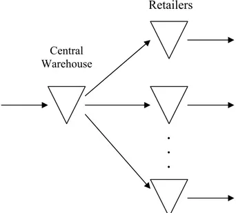
We will concentrate on the two-echelon distribution system to understand the challenges associated with a multi-echelon inventory system (see Figure 2).There are several difficulties emerging when dealing with this problem. First of all, even if the demand occurs only at the retailers and that the demand structure is known, the demand at the central warehouse is often very complicated to describe. The only easy case is when the retailers order at every customer arrival ((S-1, S) policy) and that the demand follows a Poisson process. In this special case, the demand at the central warehouse will be a Poisson process with intensity equal to the sum of all the intensities at the retailers.

. . . Central Warehouse Retailers

Figure 2: A two-echelon distribution system

A second difficulty concerns the supply lead time to the retailers. In the single-echelon system, we assume that the inventory is supplied by external suppliers who will never be out of stock. The lead time in this case is equal to the transportation time which can be considered constant in many cases. Now, the central warehouse can be out of stock, and the lead time from the central warehouse to a retailer is a random variable.

The last point to take into account is that the retailers do not react as a final customer as they can hold a stock. In most of the cases, when we consider the problem as independent single-echelon problem, the central warehouse stock level will be overestimated, as we will impose a

(14)

service level at the central warehouse much higher than optimal. This remark can be used as a rule of thumb when dealing with real problems.

1.3 The Metric approach

This approximation first developed by Sherbrooke (1968) is very useful in practice, and is also often used in research papers. The core idea of this method is to replace the random lead time to supply retailers by its mean. To well understand the method, let consider an example. We consider a two-echelon distribution system, with continuous review. We assume moreover that every location applies (S-1, S) policies and that the transportation time li for

replenishments are constant. Let assume that the demand occurring at every retailers follows a Poisson process. As explained earlier, the demand at the central warehouse follows also a Poisson process with a rate =

∑

.

iλi

λ₀

The metric approach replaces the stochastic lead time by L_i =l_i +E(W₀).Where W0 is the

time delay due to stock-outs at the warehouse. We now need to calculate E(W0). To do so, we

begin by calculating the average number of backorders at the central warehouse E(B0):

)) , 0 (max( ) (B₀ E U₀ S₀ E = −

Where U0 is the number of outstanding orders at the warehouse and S0 is the inventory

position at the warehouse.

By using the Little’s formula, it follows that:

0 0 0 ) ( ) ( λ B E W E =

From now on, we can find approximations for the average inventory on hand and the average number of backorders at retailer i.

(15)

2. Some important models

We will present in this section some important models related to our model. We will first describe the two-echelon non perishable model developed by Axsäter (1998) that we used as a starting point in our research of the perishable best policy (see Chapter 4). Then we will present some perishable models related to our study. The newsboy model is the first inventory model taking into account that the item can perish. Chiu (1995) considers a single-echelon systems dealing with continuous review (R, Q) policy and Olsson (2007b) deals with a serial two-echelon system.

2.1 Axsäter’s model

Axsäter (1998) considers a two-echelon distribution system with continuous review (R, Q) policies at every location with different reorder points and batch quantities. The retailers face different Poisson demand and the transportation times are constant. Moreover, stockouts at each location are backordered and delivered on a first-come-first-serve basis. A FIFO issuing policy is used at the retailers.

The total costs considered consist of the expected holding cost and the backorder costs at the retailers. The goal is indeed to optimize the values of R considering Q as parameters. In that way, there is no need to consider ordering costs.

In this paper, the holding and shortage costs are evaluated exactly in the case of two retailers. An approximation technique is used in the case of more than two retailers. When evaluating costs at a certain retailer, the others are aggregated into a single retailer. We will only consider the case of two retailers and mainly focus on the methodology. See Axsäter (1998) for a complete derivation of the model.

The global framework used is based on the unit tracking methodology. This method focuses on the time spent by a unit at different stages in the system from the moment it is ordered by the warehouse until it is delivered to a customer.

(16)

To keep clarity, Axsäter first uses some common assumptions that could be relaxed if needed: - The batch size at the warehouse is at least as large as the largest retailer batch size - All batch sizes are integer multiples of the smallest one (assigned to the retailer 1) - The warehouse will deliver partial orders whenever the stock on hand is not sufficient

to cover the whole batch

Axsäter first observes that there is a finite Markov chain associated with the inventory positions at the warehouse and at the retailers. This Markov chain has the properties required to conclude that the steady state distribution is unique and uniform.

Axsäter then distinguishes three different cases:

- The warehouse order has occurred before the retailer order - The warehouse order is triggered by the retailer order - The warehouse order will occur after the retailer order

The total cost is obtained by addition of the costs for these three cases.

To determine the costs for the different cases, an analogy is made with the same system but using (S-1, S) inventory policies (system where the costs are known, see Section 1.2). In the system, all units can in principle be identified as following different one-for-one policies with the aid of some probabilities. It is then possible to conclude using the fact that items following identical policies will also face the same costs.

2.2 The newsboy model

This model is the first one dealing with a perishable item. The situation is quite simple. A single vendor can order a single product (e.g. a newspaper) which will be unusable at the end of the period (e.g. one day). It is impossible to reorder during the period and the demand during this period is a random variable. On one hand, the vendor wants to maximize its revenue selling as many items as possible. On the other hand, every unsold product incurs a cost as it has to be discarded. What is the amount of items to order to maximize the profit?

(17)

Let D be the random demand during the period. Assume that D has a density function f(x) and a distribution function F(x).

If y units of the product are ordered at the beginning of the period, the remaining quantity at the end of the period (that will perish) is equal to max(0, y-D). Moreover, the unsatisfied demand during the period is equal to max(0, D-y).

Assume that every perished item incurs an overage cost of c0 per unit. The underage cost

(corresponding to the unsatisfied demand) is equal to cu per unit.

Altogether, the total cost for a period is equal to:

) , 0 max( ) , 0 max( ) (y c y D c D y C = 0 − + u − dx x f y x c dx x f x y c y C y u y 0 0( ) ( ) ( ) ( ) ) (

∫

∞ − + − =

Using the definition of f(x), we obtain:

Setting the derivative equal to 0 gives:

( )) ( ) ( ) 0 1 ( ) ( ) ( ' y =c₀F y −c_u −F y = c₀ +c_u F y −c_u = C

This gives an optimal order quantity equal to:

⎟⎟

⎠

⎞

⎜⎜

⎝

⎛

+

=

− u u

c

F

y

0 1

*

2.3 Chiu’s model

Chiu (1995) develops a model which is an approximation of the (R,Q) policy minimizing the total average cost per time unit in a single-echelon system. A continuous review policy is used and the items are considered as perishable. The demand follows a Poisson distribution and the backorders are allowed. Moreover, the issuing policy is considered to be a FIFO one. The main interest of the model is to assume a fixed non-zero leadtime L for replenishment. Chiu finds approximation for the expected outdating per order cycle, shortage quantity per order cycle and expected inventory on hand. Chiu incorporates also a fixed order cost and a

(18)

replenishment cost as the goal is to optimize both R and Q. To be able to compare Chiu’s model to both Olsson’s one and our model (where the goal is only to optimize R), we will set up these costs at 0.

Let us give some definitions from Chiu and then summarize the main results from this model. λ = demand intensity

m = Lifetime of perishable items: items are assumed to arrive fresh in inventory dL = Total demand during the leadtime L

dm = Total demand during the lifetime m

P = Shortage cost per unit W = Outdate cost per unit

ER = Expected number of units outdating of the current order size Q ES = Expected amount of unsatisfied demand during a cycle

Chiu assumes that L < m, which limits the outdating risk for the units in stock during the leadtime. The fundamental approximation in Chiu’s model is to consider that all the items on hand are still fresh when an order is placed. This assumption seems reasonable only if R is small and Q quite large.

We will not express ER here as it is quite complicated, see Chiu (1995). Chiu approximates the expected positive inventory level as followed:

2 Q L r

OH ≈ −λ +

This approximation is reasonable if Q is large enough comparing to ER and ES. The expected shortage quantity per cycle is obtained as:

L r d L d L e d L r d ES L L λ λ − ∞ + =

∑

− ≈ ₁ ! ) ( ) (

This is an underestimation of the truth since some units may have perished. The expected cycle time is approximated as:

λ

ER Q ET ≈ −

(19)

Finally Chiu express the total expected cost per time unit as: OH h ET ER W ES P Q R EAC( , )≈ ⋅ + ⋅ + ⋅

where h is the holding cost per unit and time unit. An algorithm to optimize R and Q under these approximations is then developed. We will not describe it here, see Chiu (1995).

2.4 Olsson’s model

This model is of great interest because it is, as far as we have found, the only model dealing with a multi-echelon system for perishable items with leadtimes assuming a continuous review policy. Olsson (2007b) studies a two-echelon serial system with a Poisson demand at the retailer. The issuing policy is FIFO at both locations and the unsatisfied demand is backordered. As the ordering costs are neglected, the ordering policy is assumed to be a (S-1, S) one. In opposition to what we have seen in the section 1.2, this does not imply that the demand structure at the upstream location keeps the Poisson structure. In this case, perished items must be superposed to the external Poisson demand to constitute the total demand at the upstream location. Let us give some definitions:

λ1 = customer arrival intensity at the location 1 (the retailer),

L1 = transportation time for an item to arrive at location 1 from location 2,

L2 = transportation time for an item to arrive at location 2 (which is also the leadtime as the

external suppliers are assumes to be never out of stock),

T = fixed lifetime (the product are assumed to arrive at the location 2 with a remaining shelf life of T-L2),

π1 = outdating rate at the location 1,

π2 = outdating rate at the location 2,

Whenever an item has perished, a new one is ordered. Moreover, an item is directly discarded from the stock at the location 2 if its remaining shelf life decreases to L1 since it will never

(20)

To keep clarity, we will not give all the results but we will explain the methodology used. For a complete derivation of the problem, see Olsson (2007b).

The first step is to use the result from Olsson and Tydesjö (2004) to evaluate the rate of outdating π for a single location with a Poisson demand and a fix non-zero leadtime using an (S-1, S) order policy. )! 1 ( 1 − ⋅ = − − S T e K S T λ

π

where: 1 0 1

)!

1 (

− − −

⎟⎟

⎠

⎞

⎜⎜

⎝

⎛

−

⋅

=

∫

T S t

dt

S

e

t

K

λ

The main problem when considering the two-echelon model is that the outdating rates are linked. Moreover, the demand at the upstream location is not Poisson anymore. Olsson uses several approximations in his study. First the demand at location 2 is considered to follow a Poisson process with intensity λ2 = λ1 + π1. From this point, the outdating rate at the location 2

and the steady state probability of positive inventory level can be derived.

For the location 1, the problem is more complicated. First the items which arrive do not have the same remaining shelf life. The remaining shelf life at the location 1 is indeed stochastic. Moreover, the leadtime for the location 1 is stochastic too as the location 2 can be out of stock when an order is placed. Let assume that the leadtime from location 1 to location 2 is equal to L1 + Δ. The first assumption made is that the items disappear from the location 2 according to

a Poisson process with intensity λ2 + π2. It is now possible to derive the expected density

function of Δ. Then it is possible to derive an approximation of the time an arbitrary item spends at location 2 noted W. The next step is to calculate the average residual life time when an item arrives at the location 1 Y . To do so, it is important to notice that Y =T −L₂ −W

when Δ = 0 and Y when Δ > 0. From this point, it is possible to calculate the average rate of outdating at location 1 in analogy with the location 2.

Δ + − =T L₂

(21)

Given the two outdating rate, a nonlinear system of two equation has to be solved. Olsson choose to use a numerical procedure for solving π1 andπ2. To finish, the stationary inventory

(22)

3. Literature review

The perishable characteristic of a product can affect a lot the inventory control of this product. However, the problem of considering items as perishables is a lot more complicated. From a theoretical point of view, the system has to keep track of the age of all the items until they are sold or have perished. This is certainly the reason why the literature dealing with perishable item is relatively scarce comparing to the one dealing with non-perishable items. Excellent literature reviews on perishable inventory systems are done by Nahmias (1982), Raafat (1991) and Goyal and Giri (2001). In this section, we will summarize these papers and add the literature that came out after 2001.We will first focus on the literature dealing with single-echelon systems with perishable items. Then we will consider the multi-single-echelon perishable models that can be found and we will finish referring to some related subjects when dealing with perishable items.

3.1 Single echelon systems

The main way to classify this literature is to consider if the models deal with periodic or continuous review policies.

The first papers that came out were extensions of the newsboy model. Van Zyl (1964) assumes a two-period product lifetime. Fries (1975) and Nahmias (1975) consider the multi-period lifetime case. The models become much more complex due to the size of the state space. As Nahmias (1982) points out, the three-period system is already not suitable for computations. The optimal replenishment policy depends indeed on a (m-1)-dimensional vector, which describes the age distribution of the inventory in the system. To deal with this complexity, several heuristics have been suggested for the determination of a simple ordering policy (see e.g. Nahmias (1976), Nandakumar and Morton (1993), Cooper (2001)). Under some restrictive assumptions (no leadtime, no lot-sizing and a stationary demand), these heuristic are proven to be close to optimal.

(23)

The continuous review policy received less attention. It appears that the leadtime structure is what can complicate the most in these models. When considering exponentially distributed leadtimes (or zero leadtimes), the system has a Markov property that helps a lot in the study. When dealing with deterministic leadtimes, the Markov property is destroyed and this complicates the analysis.

Let us focus on the deterministic leadtimes case. Schmidt and Nahmias (1985) consider an (S-1, S) policy with deterministic leadtime. They assume that the unsatisfied demand is lost and derive an exact result for the costs and the best inventory policy. Then Chiu (1995) consider the same model allowing backorders and dealing wit an (R, Q) policy. Approximations for holding, backorder and perished cost are derived (see section 2.3). Olsson and Tydesjö (2004) consider a model similar to Schmidt and Nahmias (1985) but assume a full backlogging instead of lost sale.

3.2 Multi-echelon systems

As for the single-echelon review, we will distinguish the periodic and the continuous review policies.

A few papers dealing with periodic review were found. The first paper dealing with multi-echelon system for perishable items is Yen (1975). For the two-multi-echelon case, he shows that the total expected outdating of stock for an order-up-to-S policy is a convex function under certain circumstances. Another interesting paper is Prastacos (1978). The same model is considered but in this paper, the emphasis is put on the allocation policy at the warehouse. More recently, Kanchanasuntorn and Techanitisawad (2006) propose a simulation study of a two-echelon distribution system with fixed lifetime and lost sales. It is shown that simple modifications to an existing model to incorporate fixed lifetime perishability and retailers’ lost sales policy improve significantly the total cost for the system. Lystad and Ferguson (2006) consider a two-echelon supply chain. Both serial and distribution systems are considered. Lifetimes and leadtimes are deterministic and the unsatisfied demand is backordered. A single-stage heuristic is developed and used to determine the stocking level for two-echelon supply chains. Some other models were developed this last decade but most of them use very restrictive assumptions.

(24)

Papers dealing with continuous review policies and deterministic leadtimes are very scarce. There exist several papers using very restrictive assumptions that are not relevant for this literature study. Abdel-Malek and Ziegler (1988) consider a two-echelon serial system and find the optimal reorder sizes with deterministic leadtimes and demand. Olsson (2007b) studies a two-echelon serial system (see section 2.4). Both locations use (S-1, S) policies. The transportation time and the products’ lifetime are fixed and the unsatisfied demand at the retailer is backordered. The demand follows a Poisson process. An approximation technique based on a variation of the Metric model is used to determine the best values of S at both locations.

3.3 Related subjects

There are some interesting subjects related to the field of perishable items that we would like to present here.

First of all, the issuing policy at the retailers becomes a major matter when dealing with perishable items. The customer is indeed very committed by receiving the freshest item. A FIFO policy is commonly used when the supplier controls the issuing policy as the LIFO policy is known to increase the perishing rate and often lowers the service level. On the other hand, customers prefer picking the freshest item first (LIFO policy) when the expiration dates are known and when it does not involve some extra cost. This is for instance the case in the supermarkets where customers can choose the product they will buy. Prastacos (1979) is dedicated to the LIFO case. Optimal and approximate solutions are found for a single-echelon perishable inventory system. Comparisons are also made with the FIFO case. Another interesting paper is Keilson and Seidmann (1990). Even if some assumptions can be seen as restrictive to allow a Markov study, it provides a wide range of numerical examples and allows a good understanding of the difference between the FIFO and the LIFO cases.

Another interesting field tries to find a replenishment policy that fits better with the perishable inventory particularities. The feeling in the papers mentioned below is that taking into account the age of the inventory into the ordering policy increase the performances of the system. Taking a simple example: If the demand intensity is 1 customer per day, do 10 units that will

(25)

perish in one day have the same utility (in term of inventory level) than 10 units that will perish in 10 days?

Tekin, Gürler and Berk (2001) compare the traditional (R, Q) ordering policy to a replenishment policy which bases replenishment decision on both the inventory level and the remaining lifetimes of items in stock. Through a numerical study, the age-based policy is shown to be superior to the stock level one mainly for slow moving perishable items with high service levels. In a working paper, Broekmeulen and Van Donselaar (2007) propose another kind of replenishment policy taking into account the age of the inventory in the system. Carrying out a numerical study, they arrive to the same results as Tekin, Gürler and Berk (2001) and they find a cost reduction of 60% for short lifetime products with low demand and high service level, when issuing policy is LIFO.

There is a last field related to the perishable inventory control that we want to present here. This field tries to find some ways to reduce the amount of waste. As Donselaar et al. (2006) points out, there are mainly three different ways to reach this goal. The first one is to reduce the leadtime to increase the remaining shelf life of the products when arriving at the retailers. For very low shelf life products, a multi-echelon inventory structure is often not relevant and direct deliveries from the producer have to be set up. The two other ways to reduce the waste of a perishable item are to limit the assortment to increase the demand rate or the use substitution. See Kök and Fisher (2007) to an in-depth study of the substitution procedure and the assortment optimization.

(26)

4. Presentation of the model

In this section, the assumptions of our model will be discussed. Then a detailed presentation of the model is presented, before describing the set of problems studied.

4.1 Assumptions

As presented in the introduction, our project consists of a simulation study. Doing so, it is possible to study very complex systems, very closed to what exists in reality. On the other hand, it is important to stay close to what is theoretically known to be able to analyze the results and draw conclusions. Moreover, this study must be helpful as a starting point to a theoretical study of multi-echelon perishable inventory systems. We took care of finding the balance between a model too complicated and a model too far away from the reality.

From a practical point of view, our main interest was the inventory control of perishable items in the supermarkets for several reasons. First the supermarket industry is one of the biggest and the inventory problems that this business faces are very interesting. Moreover, the common framework of the supermarkets’ supply chain can be well modelled as a multi-echelon distribution system (A central purchasing agency holds an inventory and distributes its products to several stores.). Finally, the perishables stand for one third of the global sales in the supermarkets (see Van Donselaar, Van Woensel, Broekmeulen and Fransoo (2006) to a comprehensive study of perishable inventory systems in supermarkets).

We will now describe the assumptions made in our model.

System structure: As explained earlier, our inspiration comes from the supermarket industry. Moreover, the aim of this master thesis is to study some kind of multi-echelon inventory systems. Hence, we decided to focus on two-echelon distribution systems. Moreover, to keep simplicity, we restricted the study at two non-identical retailers.

(27)

Number of products: As explained in the Chapter 1, there is no need to consider different products if they are not linked somehow. Moreover, our aim is not to study the assortment optimization and substitution’s problems. Consequently, we focus on a single product study. Reviewing policy: With the rise of information technologies like RFID, it is nowadays possible to get information about sales, inventory level and deliveries in real-time. We thus decided to focus on a continuous review system.

Ordering policy: In the supermarket industry, most of the products are ordered in batches. In addition, we would like to study a common ordering policy so we decided to focus on a (R, Q) policy at every location. In a lot of real cases, the batch size cannot be chosen to optimize the supply chain structure. The product’s packaging decides for us. Moreover, it would be too complicated to optimize both R and Q in a two-echelon distribution system. We set up some relevant values of Q and focus on the optimization of R at every location. With these assumptions, we discard the ordering cost from our study, as it does not affect the optimization of the reorder point.

Issuing policy: This is for us a major matter when dealing with perishable items. We thus decided to study both the FIFO and the LIFO case. Moreover, we limit our study to a First-Come-First-Serve policy at the central warehouse to keep simplicity. In addition, we assume that the warehouse will deliver partial orders whenever the stock on hand is not sufficient to cover the whole batch.

Type of perishability: As we saw in the Chapter 3, most of the studies dealing with perishable items assume that the life time is exponentially distributed. Even if this is easier to study, this does not match the supermarkets example very well. The shelf life is represented by the expiration date written on the packages in most of the cases. We therefore study the fix lifetime case. Whenever an item’s remaining shelf life declines to zero, this item is discarded. Leadtime: Even if it is much easier to neglect the leadtime when studying some perishable inventory system, it is not relevant in practice. We assume fixed transportation time in our model.

(28)

Demand structure: We focus on a Poisson demand occurring at both retailers. We set up high intensity levels to match the supermarket industry cases.

What happen when a shortage occurs: We decided to allow a full backlogging at the retailers. In practice, it is hard to decide if the customer postpones his purchase or if this one is lost when the product is out of stock. Some phenomenon of lateral transhipment can be initiated too. To keep simplicity, we use a backorder cost instead of a service level constraint.

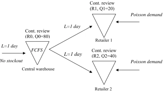
4.2 Our model Retailer 1 FCFS L=1 day L=1 day L=1 day Cont. review (R1, Q1=20) Cont. review (R2, Q2=40) Cont. review (R0, Q0=80) No stockout Poisson demand Poisson demand Central warehouse Retailer 2

Figure 3: Presentation of the model studied

- h0 = h1 = h2 = 1

- ordering costs do not enter into account

- the shelf life is calculated from the product’s arrival at the central warehouse

- The items are discarded from the central warehouse when the remaining shelf life declines to or below the transportation time to reach the retailers (1 day).

(29)

4.3 The set of problems

We decided to study a wide range of problems with both FIFO and LIFO issuing policies at the retailers.

List of the problems studied

Pb number λ1 λ2 b1 = b2 T (shelf life) p0 = p1 = p2

1 10 10 5 1,5 5 2 10 10 5 1,5 30 3 10 10 5 2,5 5 4 10 10 5 2,5 30 5 10 10 5 3,5 5 6 10 10 5 3,5 30 7 10 10 30 1,5 5 8 10 10 30 1,5 30 9 10 10 30 2,5 5 10 10 10 30 2,5 30 11 10 10 30 3,5 5 12 10 10 30 3,5 30 13 10 40 5 1,5 5 14 10 40 5 1,5 30 15 10 40 5 2,5 5 16 10 40 5 2,5 30 17 10 40 5 3,5 5 18 10 40 5 3,5 30 19 10 40 30 1,5 5 20 10 40 30 1,5 30 21 10 40 30 2,5 5 22 10 40 30 2,5 30 23 10 40 30 3,5 5 24 10 40 30 3,5 30 25 40 10 5 1,5 5 26 40 10 5 1,5 30 27 40 10 5 2,5 5 28 40 10 5 2,5 30 29 40 10 5 3,5 5 30 40 10 5 3,5 30 31 40 10 30 1,5 5 32 40 10 30 1,5 30 33 40 10 30 2,5 5 34 40 10 30 2,5 30 35 40 10 30 3,5 5 36 40 10 30 3,5 30 37 40 40 5 1,5 5 38 40 40 5 1,5 30 39 40 40 5 2,5 5 40 40 40 5 2,5 30 41 40 40 5 3,5 5 42 40 40 5 3,5 30 43 40 40 30 1,5 5 44 40 40 30 1,5 30 45 40 40 30 2,5 5 46 40 40 30 2,5 30 47 40 40 30 3,5 5 48 40 40 30 3,5 30

(30)

5. Methodology

In this section, we will focus on the methodology followed during this project. As it will be discussed later, we took a very great care of the methodology for at least two reasons. First of all, in this kind of project where simulation has a central role, the methodology used can affect the results. We will concentrate later on three different areas about the methodology which are the model validation, the process to get results from the model and the optimization process. If not taking enough care of these areas, the results from the simulation can be biased or worse completely wrong. Secondly, one of the aims of this project is to be a step stone for later studies in the field of multi-echelon perishable inventory control. From this point of view, all the assumptions have to be explained carefully. The next paragraph will explain the theoretical framework of this project. Then we will focus on the process of model validation. In a third part, we will explain how we validated the process to get information from the model and we will finish explaining how we carried out the optimization process.

5.1 Theoretical framework

First of all, it is important to mention that this project can be classified as an exploratory one. As we explain in the Chapter 3, the problem of perishable items in a multi-echelon system with continuous review is almost not studied. The project explores what happen in a situation which is not studied yet. As written in Andersson (2006) “If the research aims at seeking new insights and exploring what happens in situations not yet well understood, it is classified as exploratory. The purpose is to assess phenomena in a new light and generate ideas and hypotheses for future research.” An appropriate methodology has to be followed. As mentioned in Hillier and Lieberman (2005), the usual phases of an Operation Research project can be summarized as followed:

- Define the problem of interest and gather relevant data - Formulate a mathematical model to represent the problem

- Develop a computer-based procedure for deriving solutions to the problem from the model

(31)

- Test the model and refine it as needed

- Prepare for ongoing application of the model as prescribed by management Implement

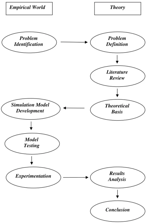
We performed some slightly changes from this methodology to fit better to our project. The Figure 4 explains the methodology used and the interactions between theory and practice in this project. Problem Identification Problem Definition Literature Review Theoretical Basis Simulation Model Development Model Testing Experimentation Results Analysis Conclusion

Empirical World Theory

(32)

To conclude this section, we would like to highlight the main idea we used about the optimization process. As we will see later, the optimization process does not reach the optimal solution, we are moreover not sure that our research method gives a solution which is closed to optimum. It is indeed very hard and time-consuming to process a full optimization as three parameters have to be optimized. However, this is not a big handicap for this project. As mentioned in Hillier and Lieberman (2005), the Nobel Laureate Herbert Simon points out that the concept of satisficing is much more prevalent in management practices in operation research. The managers seek a solution that is good enough. To quote Eilon (1972), “optimizing is the science of the ultimate, satisficing is the art of the feasible”. We could not be sure to find the optimum but we found good solutions.

5.2 Model validation

The first question that this section will try to highlight is about the advantages and drawbacks when using simulation to study a problem. As mentioned in Olsson (2007a), the main advantage of the simulation is the possibility to capture more realistic system properties without any effort. Moreover, when dealing with very complex problems as in our project, the simulation is almost the only alternative. But there are some drawbacks when using simulation. First of all, the simulation can not predict the behaviour of a system. In that sense, it is always problematical to be sure that the results are relevant. This is the main argument in favour of the use of a careful methodology when testing the model and getting the results. Interpretations of simulation results have to be done very carefully as the conclusions are only based on a number of observations and not on general results. The second problem when using simulation is about the computation-time that is often very long and can be a serious restriction.

The choice of the computer software has a lot of implications concerning the results of a project. We decided to build our simulation model using the discrete event simulation software Extend. This high level programming software allowed us to save a lot of computation time, moreover, we were able to use some models already develop. In particular, we used simulation models from Howard (2007). The problem we had to study is however not the same as in Howard’s work, but the design of the inventory system (two-echelon continuous review system) is similar. From this starting point, we modified the model to

(33)

allow items to have finite product’s lifetime. We then linked the model to the software Microsoft Excel to allow the program to collect automatically the results of the simulation and to be able to test different settings without any human intervention (see Appendix 1 for a presentation of our Extend model).

We then performed a number of tests to validate our program. To do so, we tested our program by comparing our simulation results against results obtained from some publications. Our main problem was to find relevant results to test, as almost nothing is done in the multi-echelon perishable inventory field. We decided to focus on two models. The first model that we used is a non perishable one to validate the structure of our program. We compare the simulated results from our model to the results present in Axsäter (1998).To do so, we set up the shelf life of items in our model at a very high level. Our model deals in this way with the non perishable case. We noticed that our simulation results were the same as Axsäter (1998). Our model gives good results for the total cost in the non perishable case.

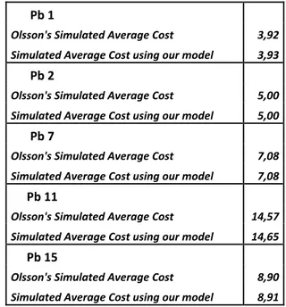
We then compared our simulated results with Olsson (2007b) (see Section 2.4) in order to validate our model. This model uses an (S-1, S) policy instead of an (R, Q) policy in our problem, but as both models are dealing with continuous review, it is possible to compare them. You can find the results in Table 2.

Pb 1 Olsson's Simulated Average Cost 3,92 Simulated Average Cost using our model 3,93 Pb 2 Olsson's Simulated Average Cost 5,00 Simulated Average Cost using our model 5,00 Pb 7 Olsson's Simulated Average Cost 7,08 Simulated Average Cost using our model 7,08 Pb 11 Olsson's Simulated Average Cost 14,57 Simulated Average Cost using our model 14,65 Pb 15 Olsson's Simulated Average Cost 8,90 Simulated Average Cost using our model 8,91

(34)

The results are also very good for all the problems tested. At that point, we were able to trust our model.

5.3 Getting results from the simulation model

The model can from now on give us good results but this always depends for a major extent of the way to use it. Three main parameters affect the results from that point of view, that is to say the number of runs per setting, the warm up period chosen and the amount of time simulated. We will now explain how we choose the values for these three parameters.

To determine the number of runs per settings, we followed Law and Kelton (2000) and calculated the average from 10 replications for each setting. In fact, as explained later, the computation-time was a matter of this project. We thus only perform one run during the optimization process using the same random seed.

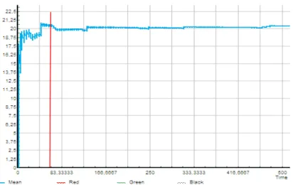
In every physical model, some time is needed before reaching the steady state. This period is known as the warm up period of the system. To determine this warm up period that we have to delete from our results, we set the model at the most variable case (low demand, high reorder points). The warm up period is due to several causes, but in our case, one simple cause is that we set up all the inventory levels at R+Q at the beginning of the simulation. The system then needs time to reach its steady state. We thus plotted all the variables of the system to see what seemed to be the warm up period. You can find one example of this in the Figure 5. The vertical line represents 50 days simulated.

(35)

Figure 5 represents one of the most extreme cases that we found. As we can see, 50 days can be considered as the warm up period. We decided to delete the first 50 days of all our simulation results.

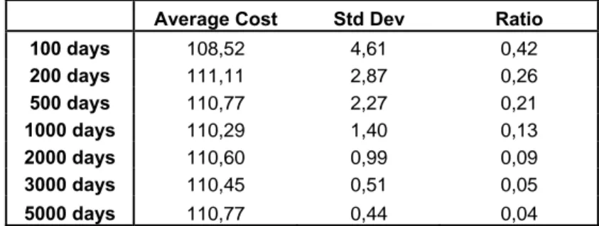
The last question we had to answer concerned the amount of time simulated. Of course, the longer is this value, the more precise are the results. But increasing it will affect the computation-time required. We thus need to find the balance between precision and computation-time. The relevant data to study this question is the standard deviation of our results. It is important to remember that the goal of our study is not to find the exact optimum for the problems chosen, we can therefore accept reasonable variations in the total cost from one run to another. We performed 10 runs simulation for several numbers of simulated days for a low demand and high reorder point problem (highest variations). The results are summarized in the Table 3.

Average Cost Std Dev Ratio

100 days 108,52 4,61 0,42 200 days 111,11 2,87 0,26 500 days 110,77 2,27 0,21 1000 days 110,29 1,40 0,13 2000 days 110,60 0,99 0,09 3000 days 110,45 0,51 0,05 5000 days 110,77 0,44 0,04

Table 3: Average Cost and Standard Deviation for different amount of time simulated

The ratio value is the proportional to 10 value of the standard deviation. It is important to notice that the simulation time is on average 2 minutes for 3000 days simulated. In that case, the value of the standard deviation is sufficiently small so we choose to simulate 3000 days deleting the first 50 days as a warm up period.

5.4 The optimization process

The problem we are facing is quite complicated from a theoretical point of view. We have to optimize the total average cost function with respect to three parameters (the value of R at the central warehouse and at both retailers). This function not proved to be convex and there does not seem to exist any easy way to find optimum. One important thing to notice is that the cost

(36)

function is very flat close to the optimum. Combining this remark with the fact that finding the perfect optimum is not the main objective of this study helped us to design an optimization process that was quick enough to be implemented for a lot of problems.

We will describe here the optimization process used for the FIFO case. The only result that can help us to start the optimization is the non perishable optimal case. As describe in the Section 2.1, the non perishable case with one central warehouse and two retailers is well studied. There exist exact and approximate results to optimize the three values of the reorder points. As our demand at the retailers is high, the exact algorithm is very time consuming. Thus we decided to use a normal demand distribution approximation at both retailers. The values of each R for this approximate optimum were used as a starting point (see Table 4).

Pb number b1 = b2 λ1 λ2 R0* R1* R2* Cost 1 … 6 5 10 10 -40 19 13 46,95 7 … 12 30 10 10 -20 19 16 63,11 13 … 18 5 10 40 -20 12 59 46,77 19 … 24 30 10 40 0 14 60 63,53 25 … 30 5 40 10 0 53 5 51,57 31 … 36 30 40 10 0 66 13 68,55 37 … 42 5 40 40 20 50 43 48,51 43 … 48 30 40 40 40 51 48 67,76

Table 4: Approximate optimum in the non perishable case

From these values, we could not predict if taking into account that items can perish tends to increase or decrease the values of R at any location. On one hand, the fact that items can perish increase the cost and the tendency will be to decrease inventory levels to lower the number of perished items. On the other hand, as items can perish, we need more items in stocks to keep the same service levels. We decided to use a [-20, +20] window from the non perishable approximate optimum and to test every combinations of R with a step of 10 units. These first 125 combinations required on average up to 5 hours computation time performing only one run per combination. It was not possible to perform more runs regarding the computation time. We thus set up a fixed random seed number to the problems. In other words, we studied only one special case of the distribution demand function. Moreover we could not be sure that the “optimum” was in that window. We could increase the step between two tested values, but this could make us missing the optimum in the window. On the other

(37)

hand, the computation time did not allow us to test more values of R in this first optimization research. This first optimization gave us a new value of a best simulated result. From this value, we performed a second research using a [-10, +10] window and we tried every combination of R with a step of 5 units.

In most of the cases studied, the optimization process seems to work well. We are not sure that we reached the theoretical optimum but we found better order policies. The process in a whole required around 10 hours computation time per problem. Our results have a precision of +/- 5 units. We finished performing 10 runs at the best simulated result found and we compared this result to the non perishable approximate optimum.

For the LIFO case, we used the same methodology but we used the best found result from the FIFO equivalent problem as a starting point.

(38)

6. Presentation and analysis of the simulation results

In this section, we analyze the results from our simulation study considering first the FIFO policy and then the LIFO one.

6.1 FIFO case

As we saw in the methodology Chapter 5, we performed an optimization process for 48 different problems in the FIFO case. The results are summarized in the Table 5.

Results FIFO

non perishable optimal Cost for this optimal perishable "optimal" Cost Pb nb R0 R1 R2 Cost Std dev R0 R1 R2 Cost Std dev % won

1 -40 19 13 150,14 0,35 -40 15 -5 142,24 0,27 5,26% 2 -40 19 13 481,73 2,20 -65 10 -10 218,80 2,18 54,58% 3 -40 19 13 92,59 0,42 -30 20 0 86,31 0,41 6,78% 4 -40 19 13 256,11 2,17 -30 10 -5 138,25 1,67 99,84% 5 -40 19 13 61,66 0,60 -30 20 10 59,68 0,44 3,20% 6 -40 19 13 135,55 1,94 -40 20 0 91,37 1,47 32,59% 7 -20 19 16 496,80 2,11 5 10 20 390,01 0,78 21,50% 8 -20 19 16 918,70 2,11 -30 15 -5 829,06 1,56 9,76% 9 -20 19 16 272,67 2,25 -10 50 50 194,71 2,93 28,59% 10 -20 19 16 515,05 3,40 -35 25 0 457,71 2,29 11,13% 11 -20 19 16 141,28 2,62 -15 25 25 127,94 4,21 9,44% 12 -20 19 16 270,90 3,73 -15 10 10 246,14 2,57 9,14% 13 -20 12 59 178,10 1,60 -50 20 80 143,20 1,33 19,59% 14 -20 12 59 580,89 4,04 -45 0 45 241,62 2,09 58,40% 15 -20 12 59 75,83 0,76 -50 15 75 65,65 0,55 13,42% 16 -20 12 59 164,17 2,82 -15 0 45 95,46 1,63 41,85% 17 -20 12 59 51,68 0,29 -30 15 65 47,30 0,15 8,48% 18 -20 12 59 63,95 0,51 -30 10 65 49,64 0,35 22,38% 19 0 14 60 545,64 3,73 25 40 75 367,86 1,24 32,58% 20 0 14 60 1243,87 9,50 5 0 30 904,16 3,66 27,31% 21 0 14 60 167,22 4,23 5 20 65 126,57 0,97 24,31% 22 0 14 60 372,88 7,18 5 15 45 290,49 4,89 22,10% 23 0 14 60 86,64 0,98 -10 15 70 75,99 0,36 12,29% 24 0 14 60 120,94 1,61 -10 10 65 95,46 0,99 21,06%

(39)

non perishable optimal Cost for this optimal perishable "optimal" Cost Pb nb R0 R1 R2 Cost Std dev R0 R1 R2 Cost Std dev % won

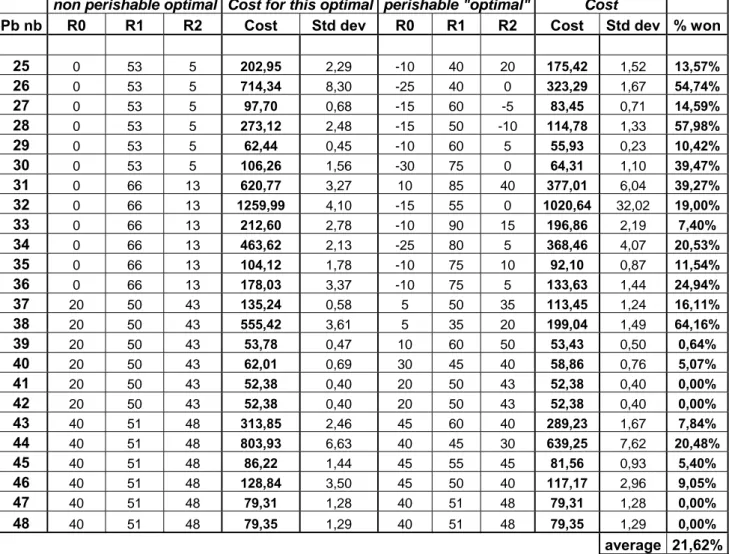
25 0 53 5 202,95 2,29 -10 40 20 175,42 1,52 13,57% 26 0 53 5 714,34 8,30 -25 40 0 323,29 1,67 54,74% 27 0 53 5 97,70 0,68 -15 60 -5 83,45 0,71 14,59% 28 0 53 5 273,12 2,48 -15 50 -10 114,78 1,33 57,98% 29 0 53 5 62,44 0,45 -10 60 5 55,93 0,23 10,42% 30 0 53 5 106,26 1,56 -30 75 0 64,31 1,10 39,47% 31 0 66 13 620,77 3,27 10 85 40 377,01 6,04 39,27% 32 0 66 13 1259,99 4,10 -15 55 0 1020,64 32,02 19,00% 33 0 66 13 212,60 2,78 -10 90 15 196,86 2,19 7,40% 34 0 66 13 463,62 2,13 -25 80 5 368,46 4,07 20,53% 35 0 66 13 104,12 1,78 -10 75 10 92,10 0,87 11,54% 36 0 66 13 178,03 3,37 -10 75 5 133,63 1,44 24,94% 37 20 50 43 135,24 0,58 5 50 35 113,45 1,24 16,11% 38 20 50 43 555,42 3,61 5 35 20 199,04 1,49 64,16% 39 20 50 43 53,78 0,47 10 60 50 53,43 0,50 0,64% 40 20 50 43 62,01 0,69 30 45 40 58,86 0,76 5,07% 41 20 50 43 52,38 0,40 20 50 43 52,38 0,40 0,00% 42 20 50 43 52,38 0,40 20 50 43 52,38 0,40 0,00% 43 40 51 48 313,85 2,46 45 60 40 289,23 1,67 7,84% 44 40 51 48 803,93 6,63 40 45 30 639,25 7,62 20,48% 45 40 51 48 86,22 1,44 45 55 45 81,56 0,93 5,40% 46 40 51 48 128,84 3,50 45 50 40 117,17 2,96 9,05% 47 40 51 48 79,31 1,28 40 51 48 79,31 1,28 0,00% 48 40 51 48 79,35 1,29 40 51 48 79,35 1,29 0,00% average 21,62%

Table 5: FIFO results

As we can see in the Table 5, some relevant amelioration can be done by taking into account that the items are perishable. Using our optimization process, our best found solution reduces the costs by more than 20% on average. That is non negligible and we can conclude that a better understanding of the multi-echelon perishable inventory systems is required. We will now analyse the results more in-depth to point out some trends of the system.

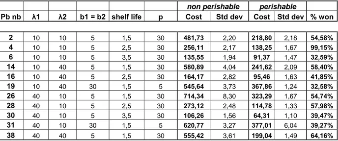
We first analysed the extreme cases in term of cost variation. We gathered the cases where the cost reduction from the non-perishable optimum is bigger than 30% (see Table 6). The best cost reduction occurs when the perishable cost is high and the backorder cost is low (p=30 and b=5). In theses cases, the perishable characteristic of the items is a crucial parameter that has to be taken into account. The two other cases where the costs reduction is bigger than 30% (problem 19 and problem 31) are with the shortest shelf life (T=1.5).

(40)

non perishable perishable Pb nb λ1 λ2 b1 = b2 shelf life p Cost Std dev Cost Std dev % won

2 10 10 5 1,5 30 481,73 2,20 218,80 2,18 54,58% 4 10 10 5 2,5 30 256,11 2,17 138,25 1,67 99,15% 6 10 10 5 3,5 30 135,55 1,94 91,37 1,47 32,59% 14 10 40 5 1,5 30 580,89 4,04 241,62 2,09 58,40% 16 10 40 5 2,5 30 164,17 2,82 95,46 1,63 41,85% 19 10 40 30 1,5 5 545,64 3,73 367,86 1,24 32,58% 26 40 10 5 1,5 30 714,34 8,30 323,29 1,67 54,74% 28 40 10 5 2,5 30 273,12 2,48 114,78 1,33 57,98% 30 40 10 5 3,5 30 106,26 1,56 64,31 1,10 39,47% 31 40 10 30 1,5 5 620,77 3,27 377,01 6,04 39,27% 38 40 40 5 1,5 30 555,42 3,61 199,04 1,49 64,16%

Table 6: Best cost reductions from the non perishable optimum

There are nevertheless 17 problems where the costs reduction is less than 10% (see Table 7). Most of these problems face either very high or very low demand rates. When the demand rates are high (λ1=40 and λ2=40), the items do not perish. That is to say that we can almost

consider the items as non perishable. The optimum in the non perishable case still holds for these problems. When the demand rate is low (λ1=10 and λ2=10), the items still perish a lot at

the best found solution. In other words, the changes of the reorder point do not have enough leverage to lower strongly the costs. In this case, the non perishable optimum is reasonable.

Perishable Items in Multi-Level Inventory Systems