J
Ö N K Ö P I N GI
N T E R N A T I O N A LB
U S I N E S SS
C H O O L JÖNKÖPING UNIVERSITYI s t h e S w e d i s h s t o c k m a r k e t
e f f i c i e n t ?
Testing the weak form of efficient market hypothesis
Master thesis within business administration (Examensarbete) Author: Lindvall, Joacim
Rangert, Fredrik Tutor: Eklund, Johan
Högberg, Andreas Jönköping May, 2012
Master thesis within Business Administration Title: Is the Swedish Stock Market Efficient? Author: Joacim Lindvall & Fredrik Rangert Tutors: Johan Ekelund & Andreas Högberg Jönköping May 2012
Keywords: Sweden, Efficient market hypothesis, Weak form
Abstract
This paper examines the efficiency of the Swedish stock market, by testing if it is possible to create an excess return by the use of technical trading rules. According to the efficient market hypothesis and the random walk theory, in an efficient market it is not possible to predict the future stock prices by analyzing historical stock prices. The profitability of tech-nical analysis and techtech-nical trading rules has been researched and debated extensively, but economists have yet to reach a consensus. Because of this we find it useful to continue to study technical trading rules, and in our case we will focus exclusively on the Swedish stock market. We have done this by applying the trading technique moving average on the Swe-dish stock exchange. We have used the OMX Stockholm 30 Index, OMXS30, the 30 most traded stocks on the Stockholm stock exchange. From Nasdaq OMX we have obtained the daily closing prices from 1986-09-30 - 2012-01-27. Our test shows support for technical trading rules. The best performing moving average is the (1,50,0), which substantially beats the buy-and-hold strategy while being statistically confident to 99%. We have also tested our data set for a unit root, if a unit root exists it implies that the data set is following a random walk. We cannot reject that there is a unit root with α = 0.10 in our data set, alt-hough it would be rejected with α = 0.11. Our result forces us to reject that the Swedish stock market is efficient which is consistent with previous research made one the Swedish stock market.
Table of Contents
1
Introduction ... 1
2
Theoretical framework ... 4
2.1 Random walk and efficient market hypothesis ... 4
2.2 What is technical analysis? ... 7
2.2.1 Moving Average ... 9
2.3 Previous research... 11
3
Method ... 16
4
Empirical findings and analysis ... 21
5
Conclusion ... 29
Definitions:
Buy and hold: A strategy based on a long position in an investment which the investor then keeps for a sufficient amount on time without trying to trade it to generate a higher payoff.
Technical analysis: A way of making future prediction of an investment based only on historical prices.
Moving average: One kind of technical analysis, by creating two different averages with different amount of data in each average. The investor then receives buy and sell signals as those lines crosses each other through time.
Technical trading: A strategy where an investor makes investment decisions based on the result of technical analysis.
Excess return: The return of an investment reduced by the return of the risk-free asset on the same period, the extra amount an investor gains due to the risk.
1
Introduction
In an effective market no one would be able to make better prediction than someone else. All information available would be reflected in the stock prices and the only way to in-crease the expected payoff is to take a larger risk (Fama, 1970). But is this really the case on the Swedish market or is it possible to gain an excess return without increasing the risk? The purpose of this thesis is to test the weak form of the efficient market hypothesis on the Swedish stock market. We are doing this by using moving average, a form of technical trading to test if the technical trading can yield a higher payoff than a simple buy-and-hold strategy. If technical trading is able to yield an excess return, the market is not efficient. Investors, within the spectrum from private persons to the largest institutions all want to receive a positive return on their invested capital. In order to make rational and informed decisions, the investor somehow needs to research the potential investment objects and evaluate this prior the investment decision. As the financial markets developed, new ways of doing the analysis also has been developed. Today, stock analysis exists in mainly two different forms; fundamental analysis and technical analysis. The first form concentrates on the financial performance of the company, the second aims to use historical information of the stock price in order to predict future stock prices. In this paper, we will focus on the technical analysis while testing if the Swedish market is in the weak form of efficient mar-ket hypothesis.
In 1970 Eugene Fama published a paper about the efficient market hypothesis. If a market is efficient in the weak form, then according to Fama (1970) it is not possible to use histor-ical stock data to predict the future stock prices. According to theories, the stock prices fol-low a random walk, and if this is true it is not possible to predict the stock prices (Malkiel, 1973).
Technical analysis has been used for centuries and is still used by analysts and stock traders in Sweden. There has been research proven that technical analysis does not beat a simple buy-and-hold strategy and therefore confirmed the weak form of efficient market hypothe-sis. Although the contrary has also been proved during the years. Major stock traders (e.g. SEB Enskilda is the largest actor on the Swedish stock market in order of volume) are us-ing technical analysis in their recommendation to their customers. So if these major
com-panies are using technical analysis there should exist a reason for this, perhaps they are even affecting the market so technical analysis is becoming self-fulfilling.
From a company‟s point of view it might not be the most interesting if it possible to make more money on their stock by active trading it than simply hold it. A company may want to find out when their stock peak, or at least not fall, in order to make it cheaper to raise new capital, although it is not their point of view we are considering. It is not the main source of obtaining capital in a company, which make that point of view less interesting.
Since technical trading cannot beat the market in the weak form of the efficient market hy-pothesis we might be able to reject that hyhy-pothesis (Fama, 1970). If we find a strategy that enables an investor to get an excess return, the market cannot be in the weak form. On the other hand, if we find that we cannot beat the market we cannot reject the weak form of the efficient market hypothesis and make a conclusion that the Swedish market is in fact inefficient.
Although the term efficient market is commonly used by researcher there is one dilemma that has not yet been solved. On what time horizon is the market efficient? Should the market be efficient for each and every second or is it efficient on a daily average? Or is the perspective longer than that, is it weekly, monthly, yearly or even longer horizon?
Furthermore we find it useful to divide the data set into shorter sub periods since previous studies indicate that smaller less developed market tend to be inefficient and more devel-oped markets tend to be more efficient. Hence markets are likely to over time move to-wards efficiency, and too old data might not be interesting for investors today. That is one of the reasons we are testing both the entire time period, to get substantial amount of data, but also divide it into sub periods to see if the market is becoming more efficient or if we can find other trends during a business cycle.
The data set is reliable since it is obtained from the Swedish stock market (Nasdaq OMX). We are although somewhat restricted with our data set and have to make a couple of as-sumptions to be able to perform our test. Since we only are able to obtain the closing pric-es of each trading day we make the assumption that an invpric-estment is made at the closing price. This might change the “real” result for an investor who is using one of these models since they are likely to make their decision perhaps six minutes before the market closes, and not at the closing second.
Dividend is simply not taken into consideration since the index never pays any dividend. Stocks that are considered in the index might pay dividend, but certificates/forward con-tracts on the index does not, hence it is not a problem in our data set.
Neither are we considering tax in this thesis, a simple buy-and-hold strategy does not gen-erate any tax obligation during the holding period. But when exiting the buy-and-hold in-vestment tax will occur (assuming the inin-vestment produced positive return). A trading model generates taxes, either by paying 30 % of the gains during the year or if the investor uses an endowment they pay a small percentage of the total value each year. Neither is a buy-sell spread taken into account which has some minor impact on the result for an inves-tor who is using moving average as a strategy, but the buy-sell spread might be seen as a part of our transaction cost which eliminates that problem.
Hence this test is not optimal for an investor who wants to replicate some of the models we are using for money making purposes, without conducting further test with more pa-rameters which is better reflecting the real scenario for an investor. The trading strategies we use are although sufficient for testing if the Swedish market is in the weak form of effi-cient market hypothesis or not.
The remainder of this thesis will in section 2 present some previous studies and theories along with some explanations within the subject. Section 3 will present our method fol-lowed by our results from our empirical findings in section 4. Finally we are drawing some conclusions of our findings in section 5.
2
Theoretical framework
There has been plenty of research in the field of market efficiency and technical trading rules. Even though this subject has been heavily debated, economists have yet to reach consensus whether financial markets are efficient or not. Efficient Market Hypothesis started to develop in the 1960s, Samuelson (1965) states that prices fluctuate randomly, and Fama (1970) developed this and formulated a definition of different levels of market effi-ciency. According to Fama (1970), in an efficient stock market historical stock data is fully reflected in the current stock prices and therefore historical prices cannot be used to fore-cast future stock prices.
In this paper we will refer to the buy and hold strategy. This strategy simply means that the investor buy a stock, and keep it in the portfolio over the entire time-period in contradic-tion to actively trade the stock in hope of maximizing the return. When evaluating the technical trading rules, we will compare the return of the trading rules with the return of the buy and hold strategy for the same index and same time period. I.e. is it possible to generate a higher return by actively trading a stock/index than to hold it over time with just one entering point and never sell it.
2.1 Random walk and efficient market hypothesis
One of the theories of the stock market is that it follows a random walk.
„A random walk is one in which future steps or directions cannot be predicted on the basis of past actions. When the term is applied to the stock market, it means that short-run changes in stock prices cannot be predicted‟. (Malkiel, 1999, p. 24) A random walk implies that each new price of a share is independent of the historical pric-es, a stock has no memory. According to Fama (1965) the theory involves two separate hy-potheses. The first is “successive price changes are independent” and the second is “the price changes conform to some probability distribution”. If the stock prices do follow a random walk, it should not be possible to use historical information to predict the future stock prices. In 1973 Malkiel published the first edition of his book “A random walk down wall street”, which made the random walk theory more widespread. Malkiel argues that even if technical analysis can make profits, in the long run the buy and hold strategy will produce higher profits. He strongly opposes the use of charts and analysing patterns in them to predict future stock movement.
In 1970 Fama published a paper regarding the efficient market hypothesis where he con-sidered both theoretical and empirical literature. According to Fama (1970) there are three states of market efficiency, weak, semi-strong and strong. He formulates three conditions for market efficiency when the current price of a security reflects all available information:
- There are no transactions cost
- All available information is costlessly available
- All agree on the implications of current information for the current price and dis-tributions of future price of each security
This is rather strong conditions, Famas comment on this is: „these conditions are sufficient for market efficiency, but not necessary‟.
The weak form test if historical prices (returns) affect future returns or if share prices fol-low a random walk. If it is possible to make an extra return by using past prices only, the market are not in the weak form. Hence, if it is possible to make an extra return with tech-nical analysis we could reject the hypothesis that a market is efficient in the weak form. The next form of the efficient market hypothesis is the semi-strong which tests the speed of adjustment of prices due to publicly available information. According to the semi-strong form all public information should be reflected in the share price and when new infor-mation are made available the logical action would be one steady jump to the new “equilib-rium” and not slowly increase/decrease step by step.
The strong form tests whether all information is fully reflected in the share price. This hy-pothesis is rather extreme since an insider should not be able to make an abnormal return due to the extra information the insider possesses. All information that is known to anyone should be reflected in the price; hence it is almost impossible for the strong form to actual-ly be fulfilled.
The weak form is the simplest and perhaps the easiest to test. You set up a null hypothesis that you cannot predict future share prices with help of historical prices. If you find it pos-sible to gain abnormal return with technical trading you could reject the null hypothesis. There are some critique against the Efficient Market Hypothesis and the Random Walk Hypothesis. Kahn (2006) argues that people are not fully rational, and when being part of a crowd they are likely follow the crowd rather than to be rational. According to Kahn this is
the explanation of bubbles and crashes in the economy. He also rejects the random walk hypothesis:
„Prices are based on calculated value modified higher or lower by human percep-tions of value. Calculated value changes in predictable ways based on the economy and the individual company. Perceived value also changes in predictable ways.‟ (Kahn, 2006, p. 9)
Lo (2004) introduces what he calls Adaptive Market Hypothesis, a version of the Efficient Market Hypothesis but which takes behavioural economics into account, Lo applies the evolutionary principles to finance. Neely, Weller and Ulrich (2007) analyse the foreign ex-change market and find support for the Adaptive Market Hypothesis. During the 2000s the field of Behavioural finance has become more accepted as an alternative to the Efficient market hypothesis. If investors are rational, and markets efficient, why does the pattern of bubbles and their subsequent crashes keep reappearing? After the recession that begun in 2007 the criticism against the Efficient Market Hypothesis, with its assumption of fully ra-tional investors, has increased (Krugman, 2009). Behavioural finance argues that the market participants are not fully rational. With this assumption, behavioural finance tries to explain some financial phenomena that the models who assumes full rationality cannot.
The foundations of behavioural finance are cognitive psychology (how people think), and the limits to arbitrage. While the assumption in Efficient market hypothesis is that the in-vestor will act rationally, studies has shown that people are subject to cognitive biases. Heu-ristics (rule of thumb), overconfidence and framing are examples of such biases. (Ritter, 2003). Limits to arbitrage refers to that the market sometimes fails to price the security at the equilibrium price.
How does algorithmic and high frequency trading affect the security markets? Although the algorithms are highly secret they have to be built on different historical data. In an ineffi-cient market technical analysis might work thus setting up algorithms that makes comput-ers trade based upon technical trading is possible to be profitable, as long as the algorithms are good. It has been a highly discussed subject if high frequency trading is good or bad for the market. According to Hendershott and Riordian (2009), algorithmic trading contributes to the efficient price since it places more efficient quotes, and by demanding liquidity to move prices towards the efficient price. Hendershott, Jones and Menkveld (2011) study in-dicate that algorithmic trading improves liquidity. Brogaard (2010) made a study on the
im-pact of high frequency trade on the U.S. equity market, one of the findings in this study was that high frequency trading did not seem to increase volatility, but rather reducing it.
2.2 What is technical analysis?
As longs as financial markets have existed, there has been a need for investors to evaluate different possible investment opportunities. There exist mainly two different forms of analysis when it comes to the stock market, fundamental analysis and technical analysis. Fundamental analysis focus on the financial performance of the company, to determine market value and future growth of the stock (Thomsett, 1998). Technical analysis uses pre-vious stock price data, in order to predict the future trend of the stock price (Park, Irwin, 2007). Investors can also combine the two kinds of analysis, first select the security by fun-damental analysis and then use technical analysis to find entry and exits points. In other words the fundamental analysis make sure that the company to invest in is in a good finan-cial shape and the technical analysis tries to gain an excess return on the stock by generate signals when to buy and sell the given stock. In that way the two form of analysis can com-plement each other in the effort to generate excess return.
Fundamental analysis is based on analysing different financial ratios, earnings, cash-flows etc. to determine the future outcomes of the company. The data can be collected from the financial statement of the company in question. Examples of usable ratios are Earnings per share, P/E, Debt ratio, Return on investment (ROI) and Profit margin (Horngren, Harri-son, Oliver, 2011). By fundamental analysis the investor can estimate the correct market value of the security, invest in this security and then realize a profit when the market adjust the price of the security towards the correct market value. Fundamental analysis is also us-able for investing with a more long term perspective (Thomsett, 1998).
Technical analysis is based on previous stock price data and tries to find trends within the movements of the stock and predict future stock price movements. Hence technical analy-sis per se does not take the condition of the company in consideration, only the past per-formance of the stock.
Technical analysis firstly appeared during the 17th century when analysts used charts to plot
the price of rice in Japan (Ahmed, Beck & Goldreyer, 2000). During late 18th and early 19th
century more research was performed and different tools were developed. When Fama formulated his efficient market hypothesis in 1970, technical analysis was losing grounds
among economists. But since the 1990s, many studies have found positive results for tech-nical trading (Park, Irwin, 2007). During the 90s, computer technology and electronic price databases became more available, and made it easier to research technical trading such as moving average.
There are many kinds of different methods within technical analysis such as chart patterns, technical indicators and trend lines. It is also possible to calculate relative strength index, different support and resistance and moving average.
It is possible to find signs in the charts by graphically study and interpret a chart of a stock price. This can be done by observing the chart and look for different patterns, and the identified pattern can give an indication of the future stock movement. The patterns have names describing their shape, such as head and shoulder, double tops/bottoms, triangles and rectangles, gaps and so on.
As discussed earlier in this paper during the review of previous research, there are many different points of view on technical analysis and its level of usefulness. By definition, the random walk and efficient market hypothesis rejects the usefulness of technical analysis: historical prices cannot predict future prices. Since Fama published his hypothesis in 1970, it has generally been accepted by economists. But in the 1990s with the paper of Brock et al technical analysis regained some popularity, when Brock et al. used trading rules to create excess return on the US stock market historical data. Their paper have been debated and Figure 1 – Head and shoulder, higher highs and lows, until the “head” is passed and the prices falls back to the headline and fail to reach the previous highs.
rejected by some and confirmed by some researchers. Since there are so many contradic-tions in matter of whether technical analysis is useful or not, the field is still interesting for further research.
2.2.1 Moving Average
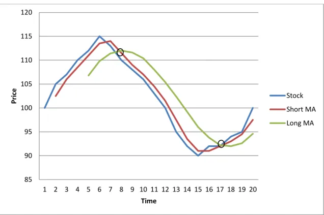
Moving average is an average of the historical prices of a stock. We are using to moving av-erage to determine when to buy/sell our index, one long and one short moving avav-erage. The short moving average uses less number of days and follows the index much closer than the long moving average which is a more smooth line and not that volatile. In figure 1 we have a stock with changes in price in every period t. We also have two different moving averages, one short and one long. The short moving average use the past two periods (t and t-1) to determine the value at time t. The long moving average use the past five periods and is therefore a much smother line since it adjusts to the stock price in a slower pace. When our two moving average crosses each other we get a signal to either buy or sell. As seen in figure 1 the short moving average is higher than the long moving average at time 5 when the long moving average first appears. At time 8 the short moving average falls below the long moving average and a sell signal appears. The sell signal indicates that we should go short in the stock and a first transaction is made. At time 17 the two averages cross and at time 18 the short moving average have risen above the long moving average thus we re-ceive a buy signal and should therefore go long in the stock until the next signal is generat-ed. This is one of the simplest methods to deal with moving average.
Figure 2 – How two moving average reacts on the change in price of a stock
Different number of days in the moving average will then generate different results, some better than others. Hence you have to test more than one moving average when testing the weak form of efficient market hypothesis. The amount of days in both the short and long moving average will affect the result. Moving averages with less number of days will be more sensitive to stock price changes, longer moving averages will not be so sensitive. There is a risk of the short moving average to fall below the long moving average but rise above quite quickly after, perhaps the as soon as the following trading day. Such short sig-nals are called false sigsig-nals. To minimize the risk of making transactions when a false signal occurs you can use a “band”. A band is a certain level of which the short moving average must increase above/decrease below in order for a buy/sell signal to occur. E.g. if the model has a band of 1 % the short moving average should be larger than the 101 % of the long moving average for a buy signal to occur. The risk of using a band is that the model might wait too long before the signal is generated hence most of the gain might have al-ready occurred when the transaction takes place. The benefit on the other hand is that less transactions leads to less transaction costs.
We find the techniques of moving average interesting to research, because it is straight forward to set up the trading rules of the selected variant of moving average. It is also straightforward to test it, by formulating the preferred rules in a spreadsheet such as
Mi-85 90 95 100 105 110 115 120 1 2 3 4 5 6 7 8 9 10 11 12 13 14 15 16 17 18 19 20 Pr ic e Time Stock Short MA Long MA
crosoft Excel and then apply them on a selected stock data set such as the Dow Jones in-dex for a specific time period. This will result in a simulated return if an investor would have followed the selected trading strategy, which is then compared to the buy-and-hold re-turn of the same stock/index. If to compare with graphical chart analysis to spot patterns as head and shoulder, moving average is not so ambiguous but it follows the trading rules of the selected moving average.
Variable length moving average (VMA) compares the two lines and when a buy signal ap-pears (short moving average > long moving average) the investor goes long in the stock/index until a sell signal appears (short moving average < long moving average) (Brock et al, 1992). When a sell signal appears the investor can choose between just selling their holdings or they could go short. If the investor chooses not to go short their money will be placed in a risk-free asset where they stay liquid until the next buy signal. With VMA all days are label either buy or sell days.
The theory behind fixed moving average (FMA) is that there will be an increase (decrease) when the short moving average goes above (below) the long moving average for a couple of days (Brock et al, 1992). Hence, if a buy signal occurs you go long in the stock for a fixed number of days and during that time ignoring other signals. After the given days have passed the investor liquidates the investment and invests in a risk-free asset until the next signal occurs.
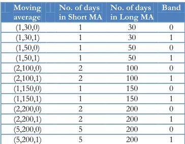
A moving average model with 1 day in the short moving average, 50 in the long moving average and 1 % band would then look like (1,50,1).
2.3 Previous research
Fama and Blume (1966) tested the US stock market with the filter rule technique and Jen-sen and Benington (1970) used relative strength to test 200 securities on the N.Y.S.E, and they find that when taking transaction cost into account, technical trading generates no ab-normal profits. Both these studies agreed on that it was not possible to make a significant profit from this technical analysis.
By the end of the 1970s scholars seem to reject technical trading (Metchalchi, Chang, Maraucci, 2007). But Sweeney (1988) finds support for technical analysis, and in 1992 Brock, Lakonishok and LeBaron published a now very well cited paper.
„Technical trading has been enjoying a renaissance on Wall Street. All major broker-age firms publish technical commentary on the market and individual securities, and many of the newsletters published by various “experts” are based on technical anal-ysis.‟ (Brock et al, 1992)
They test some of the simplest and among stock trader‟s most popular trading rules, the moving average and trading range break. Important to keep in mind is that the brokerage firms have some incentive to publish buy and sell recommendations, since this generates revenue for them in the form of transaction costs paid by the investors. The data they use is the Dow Jones index from 1897-1986, and their conclusion is strong support for tech-nical analysis ability to create excess return. Brock et al. concludes that the average buy-and-hold return is about 5%, and their best performing tested trading rules create a return of 12%. However, this return is without taking transaction cost into account, which the au-thors advice careful consideration of before implementing technical trading strategies. Hudson, Dempsey & Keasey (1996) research the UK market and reject that the findings of Brock et al can be applied on the UK market. Bessembinder & Chan (1998) extend the Brock et al analysis, and confirm their basic results but argue that this can coexist with market efficiency. They also argue that when taking transaction costs into account the in-creases in portfolio return from technical trading would diminish.
Ahmed, Beck and Goldreyer (2000) test moving average on three emerging Asian markets. They use data 1994-1999 from Taiwan, Thailand and Philippine stock exchanges, all three markets having a declining trend during this period. They find strong positive results for variable moving average in these emerging and volatile markets. When comparing two more developed markets, US S&P500 and Japan JP225, they fail to create abnormal return. According to them this is because technical analysis is more useful on an inefficient market and not useful on the more efficient Japan and US markets.
Gunasekaragea and Power (2001) found that by using moving average techniques, an inves-tor gained excess return to a buy and hold strategy in four different South Asian markets, and concluded that these are not in the weak form of efficient market hypothesis.
Allen and Karjalainen (1999) develop some technical trading rules in order to test if they can create excess return, but find no strong support for technical analysis on the US stock market. Ready (2002) examines the conflicting results of Allen et al and Brock et al. Ready argue that:
“This comparison lends support to the hypothesis that the apparent success (after transaction costs) of the Brock et al. (1992) moving average rules is a spurious re-sult of data snooping”. (Ready, 2002)
Because Brock et al. choose trading rules popular among the 1980s analysts, the result of Brock et al. might be from a spurious of data snooping. Data snooping occurs when the same data set is used several times. Ready‟s conclusion is that the trading rules of Brock et al. performs badly after 1986 when tested on stock data from 1987-2000. He argues that a investor about to invest in 1963 and who are looking back on the 1945-1962 data cannot find any rational reason to choose the trading rules of Brock et al., and thus the reasons for choosing the Brock et al. rules “is only clear for researchers examining the price data ex-post”.
Looking at research done on the Swedish market, Jennergen and Korsvold (1974) test the random walk hypothesis on the Norwegian and Swedish market and Frennberg and Hans-son (1993) test only the Swedish market. The studies reject the random walk hypothesis for both the Swedish and Norwegian markets. Metghalchi, Chang and Marcucci (2008) test some technical trading rules on the Swedish market, with data from OMXS30 1986-2004. To mitigate the problem of data snooping, they adopt a test developed by White (2000), called Reality check. They find support of profability for some of the rules they tested, also when taking transaction cost into account. When considering transaction costs, they find that the model of Increasing Moving Average generates significant excess return, but the Arnold and Rahfeldt Moving Average (1986) create too many trades which reduces the profit. They formulate a strategy of taking a loan to double the stock investment during buy days, and combining this with the trading rules of Moving Average. According to their research, this strategy “significally beats the buy-and-hold strategy”.
Allergren and Sundberg (2009) also research the usefulness of technical analysis on the Swedish stock market. They find that the Weighted Moving Average (WMA) 20-50 with 1% band, gives excess return and correct buy/sell signals also when taking transaction costs into account. They split the dataset into sub periods, and find that moving average is less useful during periods with lower volatility. Stronger trends suit the moving average technique better. They find support for the possibility that moving average can create ex-cess return on the Swedish market, but advice caution for investors. They conclude that
moving average can be used as a trend indicator, but it should be used together with other analysing tools.
Table 1 – Summary of previous research
Publication Conclusion
Fama and Blume (1966) Jensen and Benington (1970)
No significant profits from TA when taking transaction cost into account
Sweeney (1988) Support for TA
Brock et. al. (1992) Strong support for TA, cited ~1200 times
Hudson, Dempsey & Keasey (1996) Applies Brock e. al. on UK market, no TA support Bessembinder & Chan (1998) Extends Brock e. al. on UK market, supports TA Allen and Karjalainen (1999) No strong support for TA on US market
Ready (2002) Compares Allen & Karjalainen. & Brock et al.: supports Allan & Karjalainen.
Ahmed, Beck and Goldreyer (2000)
Gunasekaragea and Power (2001) Support for TA on emerging Asian markets Jennergen and Korsvold (1974)
Frennberg and Hansson (1993) Swedish market does not follow a random walk Metghalchi, Chang, Marcucci (2008) Support for TA on Swedish market
One of the issues with trading rules such as the moving average is that it is often hard to know which set of rules to use prior the investment. In many studies researchers post ana-lyze data by applying a number of technical trading rules. The result are often that some of the trading rules are proved to be profitable, thus beating the buy-and-hold strategy, and some of the trading rules fatally fail to beat the buy-and-hold strategy. For anyone who post analyze, as the researchers normally do, it is easy to conclude that a specific trading rule generate an excess return. But what we have seen during our review of previous re-search, depending on which market and which state the economy is in it often differs which trading rule that have the ability to create excess return! As Ready (2002) comments on the Brock et. al paper, there was no apparent rational reason to choose the trading rule
Brock et. al. proved to be profitable. Ready claims this choice is only clear when post ana-lyzing the data, an opinion we share and have observed in a number of other studies. An-other issue is the matter of data snooping, it occurs when the same dataset is re-used in many studies, and when reusing this can create a biased result. When these kinds of studies are performed, the researchers are forced to re-use data, since is simply only one Dow in-dex available so this makes it more or less impossible to find new data. Hsu and Kuan (2005) re-examines some previous studies and check for data snooping. They find signifi-cant profitable trading rules in what they call young markets (Nasdaq composite, Russel 2000) but not in more mature markets as Dow Jones Ind. Average and S&P 500.
3
Method
By taking the view of an investor we need to face transactions cost and our objective is to make a better payoff after these transaction costs are paid, then we would if we just bought the stock at day one and hold on to it. We will assume a transaction cost of 0.075 % per transaction, which on a day where we both buy and short sell will imply a total transaction cost of 0.15 %. The transaction cost is based upon what a small or medium sized investor could face in Sweden at one of the largest internet brokers. A larger investor may face even lower transaction cost than we are using, but to make the result interesting for as many as possible we choose 0.075 %.
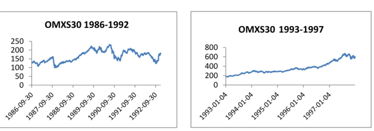
The data (closing prices of OMX Stockholm 30 Index, OMXS30) is obtained from Nasdaq OMX´s website, from 1986-09-03 until 2012-01-27. The data of the risk-free rate are ob-tained from the Riksbank‟s website. We are conducting tests of different moving averages and divide our sample into five subsets with a number of years in each set to see if we might find some patterns that changed during the years. Hence, we are only dealing with secondary data, but which we find reliable. Figure 3 shows the development of the Swedish stock market during the time period we are interested in.
Figure 3 – The price of OMXS30 during our entire test period
0 200 400 600 800 1000 1200 1400 1600 1800
OMXS30 1986-09-30 - 2012-01-27
We are dividing the full period into five smaller sub periods to be able to find differences between them. In table 2 we describe our different sub periods. And the diagrams below show how the market has moved in the different periods.
Table 2 – Description of sub periods
Sub period Description
1986-09-30 – 1992-12-31
During this period the market were quite volatile with both ups and downs without a clear pattern. Although the market did rise during this period. At the beginning of the 90‟s there was a banking crises which created uncer-tainty which shaped the market.
1993 – 1997 Already in the second half of 1992 the market started to climb, which then characterized the market for the following years. The late 90‟s was also the start of the dotcom bubble which later crashed in the beginning of 2000. 1998 – 2002 The first half of this period was just before the dotcom bubble broke which
meant a lot of positive days on the market, but when the bubble broke a long and intense fall begun. This period was suffering from declining prices on the stock market.
2003 – 2007 At 2003 the market started to rise again and next few years follows the same patterns as we saw in our third set with a nice upward going trend. 2008-01-01 –
2012-01-27
The last period in our subset does not have a clear trend and is once again quite volatile and the last day is just below our first day. The mayor event during this period is the financial banking crises which started with some bad housing loans in the USA which lead to the bankruptcy of Lehman Brothers Ltd.
The diagrams below illustrate the trend for each period. By dividing our data into different sub periods we can identify how the market trend influence which of the trading rules that produce the highest return.
0 200 400 600 800 OMXS30 1993-1997 0 500 1000 1500 2000 OMXS30 1998-2002 0 500 1000 1500 OMXS30 2003-2007 0 500 1 000 1 500 OMXS30 2008-2012 0 50 100 150 200 250 OMXS30 1986-1992
Figure 4 – First sub period Figure 5 - Second sub period
Figure 6 – Third sub period Figure 7 – Forth sub period
Table 3 – Variable length moving average models
A moving average model with 1 day in the short moving average, 50 in the long moving average and 1 % band would then look like (1,50,1). We are using the same variable length moving average as Fiefield, Power and Sinclair (2005) did in eleven other European mar-kets. We are also testing (1,30,0) and (1,30,1) to see if a smaller number of days in our long moving average will be a better prediction of future returns.
We have found that variable length moving average is often used in similar studies done in the past and in other markets. We do not think that a more advanced model is always bet-ter to predict future market movements. The more simple the model the easier it is to un-derstand and use for an investor, that is another reason why variable length moving average is popular. With fewer parameters the human error factors heavily diminish and the risk of wrongly interpret the data and the result. The different moving averages we are using are shown in table 3. The first column displays the amount of days in the short moving aver-age, the second column shows the amount of days in the long moving average and the third column shows the band. Each row is a separate model we are using.
The return on a given buy day are calculated by the given formula: ( )
Where Rit is the return on the index at day t, ln is the natural logarithm, Pit is the closing
price on index at day t and Pit-1 is the closing price on the index the day before day t.
The return on a given sell day (in case of short selling) is then the opposite:
Moving
average No. of days in Short MA No. of days in Long MA Band
(1,30,0) 1 30 0 (1,30,1) 1 30 1 (1,50,0) 1 50 0 (1,50,1) 1 50 1 (2,100,0) 2 100 0 (2,100,1) 2 100 1 (1,150,0) 1 150 0 (1,150,1) 1 150 1 (2,200,0) 2 200 0 (2,200,1) 2 200 1 (5,200,0) 5 200 0 (5,200,1) 5 200 1
( )
We are then testing the statistical significance on each sub period and the whole period by making a linear regression on the excess return on the index versus the excess return on our trading, considering transaction costs. The excess return is the return on the invest-ment reduced by the return on the risk-free asset. The regression is made on the excess re-turn on the index and the excess rere-turn on the trading strategy. So it is the two different excess returns that are compared. The excess return is calculated as follows:
Where Rft is equal to the daily risk-free rate at time t. We are using the Swedish 30-days
T-bills interest as our risk-free rate.
We are formulating a null hypothesis which we are testing.
H0 = The Swedish stock market is in the weak form of efficient market hypothesis.
HA = The Swedish stock market is not in the weak form of efficient market hypothesis.
Our regression estimates if the result is reliable or not and we are using t-tests with α = 0.1, α = 0.05 and α= 0.01 to find the statistical significance.
We will also be testing for a random walk in our data set. We are using a unit root-test to find if our time series are following a random walk which would imply that technical trad-ing will not be able to predict future price movements.
4
Empirical findings and analysis
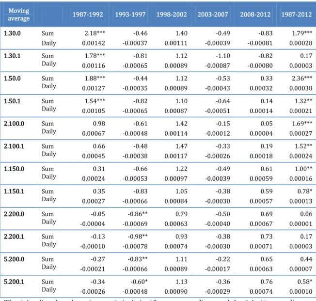
Table 4 and 5 displays the results, logarithmic return, for our twelve tested trading rules. The data is separated in five sub periods, and the last column display the result for the full time period 1987-2012. Table 4 displays the excess return and column 2 indicate if the row is displaying the total excess return for the period or the daily average excess return for the period. In the first row, total excess return:
∑
While the second row is showing the average daily excess return: ∑
As shown in table 4, each moving average indicates excess return in the last column but only a couple of them have statistical significance with alpha 1 % and 5 %, mostly the shorter ones. Another interesting trend is that the smaller moving averages was better than the larger ones during our first sub periods but during the last sub periods the larger mod-els have been the better ones, although this conclusion lack statistical significance.
In table 4 the excess return compared to the buy-and-hold strategy is presented. For each moving average the sum is presented in the first row and the average daily excess return is presented in the second row for each sub period and the entire period. The excess return is calculated, as mentioned earlier, as the return with trading reduced by the return for the buy-and-hold strategy. Hence, if the excess return is minus it does not necessarily implies that a portfolio using that moving average has decreased, but it has performed worse than the buy-and-hold strategy.
Table 4 – Excess return technical trading compared to buy-and-hold Moving average 1987-1992 1993-1997 1998-2002 2003-2007 2008-2012 1987-2012 1.30.0 Sum Daily 2.18*** 0.00142 -0.46 -0.00037 1.40 0.00111 -0.49 -0.00039 -0.83 -0.00081 1.79*** 0.00028 1.30.1 Sum Daily 0.00116 1.78*** -0.00065 -0.81 0.00089 1.12 -0.00087 -1.10 -0.00080 -0.82 0.00003 0.17 1.50.0 Sum Daily 0.00127 1.88*** -0.00035 -0.44 0.00089 1.12 -0.00043 -0.53 0.00032 0.33 0.00038 2.36*** 1.50.1 Sum Daily 0.00105 1.54*** -0.00065 -0.82 0.00087 1.10 -0.00051 -0.64 0.00014 0.14 0.00021 1.32** 2.100.0 Sum Daily 0.00067 0.98 -0.00048 -0.61 0.00114 1.42 -0.00012 -0.15 0.00004 0.05 0.00027 1.69*** 2.100.1 Sum Daily 0.00045 0.66 -0.00038 -0.48 0.00117 1.47 -0.00026 -0.33 0.00018 0.19 0.00024 1.52** 1.150.0 Sum Daily 0.00024 0.31 -0.00053 -0.66 0.00097 1.22 -0.00039 -0.49 0.00059 0.61 0.00016 1.00** 1.150.1 Sum Daily 0.00027 0.35 -0.00066 -0.83 0.00084 1.05 -0.00030 -0.38 0.00057 0.59 0.00013 0.78* 2.200.0 Sum Daily -0.00004 -0.05 -0.00069 -0.86** 0.00063 0.79 -0.00040 -0.50 0.00067 0.69 0.00001 0.06 2.200.1 Sum Daily -0.00010 -0.13 -0.00078 -0.98** 0.00074 0.93 -0.00030 -0.38 0.00071 0.73 0.00003 0.17 5.200.0 Sum Daily -0.00021 -0.27 -0.00066 -0.83** 0.00089 1.11 -0.00017 -0.22 0.00063 0.65 0.00007 0.44 5.200.1 Sum Daily -0.00026 -0.34 -0.00048 -0.60* 0.00090 1.13 -0.00029 -0.36 0.00074 0.76 0.00010 0.58*
The * implies that there is a statistical significance according to alpha 0.1, ** according to alpha 0.05 and *** to alpha 0.01.
During both of the sub periods with clear upward trends (1993-1997 and 2003-2007), we have a similar pattern where no model beats the buy-and-hold strategy and yields excess re-turn. But then there are opposite results when the stock market lacks a clear trend and in our third sub period (1998-2003) all the moving averages shows an excess return, in the first period (1986-1993) all but the largest moving average (2,200,0/1) shows excess return and in the last period (2008-2012) it is only the smallest moving average (1,30,0/1) that does not yield an excess return. It is not surprising that trading stocks actively is less bene-ficial during bullish markets since it is increasing the “risk” of missing upturns in the stock market. A bad signal does not only generate a negative payoff, is also decreases the invest-ment due to transaction costs. When the market is not in a bullish trend, perhaps if it is in a bearish trend, it is beneficial to move out of the market for some time and even to be short
selling assets. A good short sell is in a way twice as good as a regular investment since the investor does not only avoiding the drop but also making money out of it. When compar-ing a tradcompar-ing strategy with the buy-and-hold strategy on the same asset it is only the days out of the market, or in our case the days we are short selling, that may yield a positive ex-cess return. On a given buy day our portfolio increases/decreases exactly as much as the benchmark which does not yield an excess return. That is the main reason that it is difficult to yield excess returns during bullish markets, even though a positive payoff is still ob-tained.
Hence, the Swedish stock market seems to have changed. The best moving average for predicting future returns have changed from a small moving average to a larger moving av-erage, but once again this lack statistical evidence. For an investor trying to create an excess return with these methods this is not favorable. Since which moving average that works best is constantly changing the investor cannot know for certain which will be the best for the next few years. Although the pattern does not change that fast, the model that was best in one period is also in the top in the next period hence the investor can choose the one that was best in the previous period.
The strategy that has yield the largest excess return during the entire period is (1,50,0) and is statistical significant with a confidence interval of 99 %. Both (1,30,0) and (1,30,1) did very well in the first period (1987-1992) but comparing the first period with the total period there is a clear pattern of decline even though they were both performing well under the third period (1998-2002). The exact opposite goes for the larger moving averages which did not perform well during the early 90‟s but has been outperforming shorter ones during the two last periods (2003-2012). Using 200 days in the long moving average combined with a one percent band has proven to yield the highest excess return since 2003.
Table 5 shows the average daily return on a given buy day on the first row and a given sell day on the second row for each model and sub period. The return on sell days is the return for an investor whom has chosen to short sell, which means that the return on the index is the opposite of the table. As seen in the last column for each and every model the average return on a buy day have been better than on a sell day during the whole period. That is not surprising though since the market has increased a lot since 1987. The negative returns (loss for investors) are more likely to appear when a sell signal has occurred than when a buy signal has occurred which make short selling less attractive. In other words if you only
choose between going short or going long it is preferable to go long. Although going short have in many cases proved to yield positive payoff as well. For most models it is during 1993-1997 and 2003-2007 that short selling has yield a negative return, the periods with bullish markets. For most models, all but (2,200,0) and (2,200,1), short selling has yield an average positive return for the investor during the whole period.
Table 5 – Average daily returns divided on buy and sell days
Moving average 1987-1992 1993-1997 1998-2002 2003-2007 2008-2012 1987-2012 1.30.0 Buy Sell 0.00162 0.00162 0.00123 -0.00072 0.00075 0.00117 0.00079 -0.00095 -0.00094 -0.00072 0.00081 0.00031 1.30.1 Buy Sell 0.00141 0.00133 0.00103 -0.00119 0.00020 0.00133 0.00041 -0.00160 -0.00075 -0.00094 0.00056 0.00004 1.50.0 Buy Sell 0.00149 0.00166 0.00102 -0.00050 0.00056 0.00093 0.00060 -0.00083 0.00012 0.00051 0.00082 0.00055 1.50.1 Buy Sell 0.00129 0.00133 0.00088 -0.00125 0.00051 0.00089 0.00065 -0.00102 -0.00004 0.00029 0.00072 0.00026 2.100.0 Buy Sell 0.00103 0.00068 0.00093 -0.00139 0.00080 0.00111 0.00080 -0.00032 -0.00023 0.00031 0.00074 0.00036 2.100.1 Buy Sell 0.00062 0.00082 0.00103 -0.00126 0.00065 0.00132 0.00075 -0.00068 0.00013 0.00016 0.00069 0.00038 1.150.0 Buy Sell 0.00065 0.00011 0.00078 -0.00141 0.00057 0.00093 0.00070 -0.00124 0.00038 0.00071 0.00065 0.00019 1.150.1 Buy Sell 0.00052 0.00032 0.00074 -0.00207 0.00052 0.00072 0.00065 -0.00069 0.00028 0.00078 0.00058 0.00021 2.200.0 Buy Sell 0.00047 -0.00021 0.00080 -0.00517 0.00040 0.00049 0.00051 -0.00090 0.00050 0.00079 0.00057 -0.00010 2.200.1 Buy Sell 0.00039 -0.00023 0.00067 -0.00455 0.00042 0.00068 0.00061 -0.00075 0.00060 0.00073 0.00056 -0.00003 5.200.0 Buy Sell 0.00031 -0.00027 0.00061 -0.00270 0.00044 0.00095 0.00061 -0.00012 0.00063 0.00056 0.00054 0.00018 5.200.1 Buy Sell 0.00028 -0.00032 0.00087 -0.00344 0.00062 0.00080 0.00065 -0.00079 0.00055 0.00086 0.00063 0.00007
As in table 4 we can confirm that the two shortest models (1,30,0) and (1,30,1) have not been beneficial in the last two periods (2003-2007 and 2008-2012), where neither the buy nor the sell signals have generated a positive payoff in the last period (2008-2012). The model that yield the best excess return (1,50,0) has only two periods with negative pay off for short selling, period 1993-1997 and 2003-2007. Furthermore all the buy signals generat-ed by (1,50,0) have a positive payoff. In the three periods 1987-1992, 1998-2002 and
2008-2012 the sell signals have generated a positive return and the average return have been larg-er then on the buy days. This implies that short selling is an important part of the model. If our moving average models would not be able to predict future returns there would not be a difference on average return on a given buy day or a given sell day. Since in table 5 we find that in almost every model yields a positive payoff on both buy and sell days (all but two models) there certainly is a difference which supports our results that technical analysis in fact may predict future returns.
Consider that two investments were made when the first signal was generated by the (1,50,0) strategy, one which would be using a buy-and-hold strategy and the other would be using the signals generated by the moving average. During the next approximately 24 years which our study is covering the return from the buy-and-hold has increased by 8.7 times the original investment. The trading strategy on the other hand would have increased by 27.3 times the original investment. Hence it has been a huge difference for investors who have traded their investment with a good strategy comparing those who have let their in-vestment be still for the entire period.
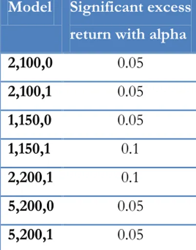
If a market is inefficient that implies that an asset is not always priced at its true value, it may be both underpriced and overpriced. Since assets may be wrongly priced it is not only possible for an investor to make an excess return, investors might lose more/gain less than warranted by their risk profile. That is one of the reasons that it is preferable to invest in a more efficient market, due to a higher level of risk control in a more efficient market. But according to these result, the most of the excess return seems to appears in the first pe-riod. Has technical trading not been profitable since then? We choose to test our strategies after the two first period and tests from 1998-2012 to find out if our trading rules have provided a statistical significant excess return during that period.
According to our test we find that some of our models have provided an excess return with statistical significance. The result is presented in table 6, it shows in which level of alpha each model is statistical significant.
Table 6 – The models with excess return 1998-2012
Model Significant excess return with alpha
2,100,0 0.05 2,100,1 0.05 1,150,0 0.05 1,150,1 0.1 2,200,1 0.1 5,200,0 0.05 5,200,1 0.05
Hence, technical trading rule has been efficient even after 1992.
We perform a test to find if our time series has a unit root. If a unit root exists it would not be possible to use technical trading to make an excess return, since the data would follow a random walk. We are using the formula:
Where we formulate the hypothesis:
H0: (unit root exists, hence, random walk). HA: (no unit root exists, hence, no random walk).
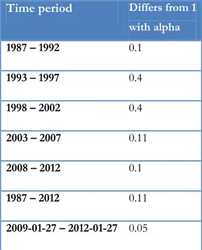
Our beta differs slightly from 1 but without statistical significance at the 90 % confidence interval. So we cannot reject that there is a unit root in our full data series which is contra-dicting to our previous results. With a unit root the random walk hypothesis holds which would then imply that the weak form of efficient market hypothesis also holds.
Table 7 – Unit root test for our sub periods
Time period Differs from 1
with alpha 1987 – 1992 0.1 1993 – 1997 0.4 1998 – 2002 0.4 2003 – 2007 0.11 2008 – 2012 0.1 1987 – 2012 0.11 2009-01-27 – 2012-01-27 0.05
On the other hand when testing the last three years instead of the entire time period we find that our β < 1 which is statistical significant at the 95 % confidence interval. Hence, the market does not seem to follow a random walk at all times which make it possible to create an excess return in between. We test for a unit root in all of our sub periods and find that we can actually reject that there is a unit root in the first and last sub period at α = 0.1. The other three sub periods has a beta that differs from 1 but not with enough statistical significance. Although the forth sub period and the full period is almost rejected as well, with α = 0.11 they would be rejected hence there is no clear evidence for a unit root. Our result after testing the profitability of technical trading is therefore supported by our unit root test. The result that it is possible to create an excess return on the Swedish market by technical trading is also consistent with the result of the Metghalchi et al. (2008) study on data until 2004.
For a market to become efficient it is, ironically, important for people to believe in an inef-ficient market. When people try to exploit mispricing in the market they drive the market to efficiency. On the other hand if people tend to believe that the all information is fully re-flected and do not try to exploit mispricing assets might stay mispriced leading to ineffi-ciency. The wheel then goes round and round and the market will never be fully inefficient or efficient.
The technology with computers and high frequency traders are making the market more ef-ficient which is most likely one of the reasons that our largest excess return is in the first sub period. Today it is easier for investors to gain information at lower cost (both in terms of time and money) and making analysis becomes easier in a way for the investors. The al-gorithmic traders are offering a more liquid market which makes it less volatile and pushes prices faster to their true values exploiting mispricing.
If a market is inefficient this implies that an asset is not always priced at its true value, it may be both underpriced and overpriced. Since assets may be wrongly priced it is not only possible for an investor to make an excess return, investors might lose more/gain less than warranted by their risk profile. That is one of the reasons that it is preferable to invest in a more efficient market, due to a higher level of risk control in a more efficient market. In an efficient market where assets are priced at its true value bubbles should not occur nor would financial crashes on the stock market. Of course a market could rise or fall quite heavily at times, but the tops would not be as high and the bottoms not as low as the case in an inefficient market. In bubbles investors tend to pay overprice compared to a true val-ue, in crashes investors tend to sell at underprice. That a market is not strong efficient is understandable since not every investor has the same information and different investors tend to evaluate the same information differently. Although that alone would not lead to these bubbles and crashes. It is argued that during bubbles investors follow the crowd, eve-ryone believes in future rise which during some time might be right, until the price hits the ceiling. When the top is reached the mood of the crowd suddenly changes and the inves-tors starts to sell, perhaps even in panic, which then pushes the price below its true value. Neither the rise nor the fall should happen in an efficient market. The only time a stock would move, significantly, is when new information is revealed. In a perfect market stock charts would look like they were drawn with a ruler, a flat line where the stock makes sud-den jumps up or down. But even if the market is not perfect, in the weak form of efficient market hypothesis the stock chart would be less blurry then they tend to be today.
5
Conclusion
From our research we find that by using moving average without a band and 1 day in the short moving average and 50 days in the long moving average (1,50,0), the market would have been outperformed during our sample period. This is statistically significant at α = 0.01. The excess return by trading is significantly larger than the excess return on the index. Hence we can reject that the Swedish stock market is weak efficient. Since the weak form is not fulfilled nor can the semi-strong or the strong form be fulfilled, hence the Swedish stock market has been inefficient when using daily closing prices during the last 25 years. Although we can find a unit root in some sub periods and during the entire periods, we al-so find a lack of unit root during al-some time periods. This combined with statistically signif-icant excess return from technical trading, allows us to find our result reliable. Our result is also consistent with previous research on older data on the Swedish stock market.
Our result is also strengthen when testing the market from 1998-2012 which proves that it is just not the first sub period that generates an excess return. The consistent result where we both find periods that does not follow a random walk and that we can generate a statis-tical significant excess return with technical trading rules make us confident in our result. The inefficiency on the Swedish market proves that historical prices could be helpful in in-vestment decisions for an investor‟s point of view. That the market is inefficient also ex-plains why high frequency trading could work the Swedish stock market.
The main reason for market inefficiency is perhaps not that investors has different infor-mation and/or make different analysis with the inforinfor-mation they possess. People are not rational at every point in time in their investment decisions. The result of our research is supporting the theories of the adaptive market hypothesis and behavioral science, the effi-cient market hypothesis is perhaps not the best way of describing markets.
We do not believe that transaction cost should be a reason for market inefficiency since they have declined a lot since the middle of 1990´s and are today so low that they have very small impact on returns. And even though transactions would be high it does not imply market inefficiency. When we are testing the market transaction cost is in fact lowering our return on the trading strategies which lowers the excess return compared to a simple buy-and-hold strategy. Hence transaction cost is in our testing working for market efficiency, not against.
Considering that which moving average generates the best excess return changes from one sub period to another it makes it more difficult to choose which moving average to use. How long should an investor hold on to the same moving average and which one should the investor choose? If an investor always use the same for a e.g. five year period, should the investor then change to the one who has been most effective during the last five years for the next coming five years? And which time horizon is working best? If it is too long the investor might fall behind, but if it is to short it might be too many changes which lead to inaccuracy. From our sub periods we find that the moving average that was best in one sub period is not the best in the next, but it seems to always be in the top. So even though the market is moving, it does not move too fast for an investor to be able to change their strategy.
Further research could focus about how an investor could best benefit from using the in-formation of the inefficiency on the Swedish stock market. Our research has proven the ef-fectiveness of variable length moving average and more combinations could be tested with-in that strategy.
Also fixed length moving average could be used. To find the best amount of days to use in fixed length moving average (different amount of days could be used for buy respective sell signals) further research could test the average return after a buy/sell signals is received. Watching the average return after a signal will indicate how many days to use in a technical trading strategy.
Research could not only be focusing on how investors may take advantage on the tiveness on the market, but also what parameters that makes the market stay in the ineffec-tive state. Sweden is a developed country with large international firms, how come it has not reached the weak form of efficient market hypothesis.
Another aspect could be to test the Swedish market with weekly data or monthly data to see if the results differ when a larger interval between the observations is used. Also it would be interesting to see if similar study is made on mid cap and small cap on the Swe-dish stock market. Are smaller companies more or less efficient? Since less developed mar-ket tends to be less efficient one could assume that small cap should be even less efficient than large cap or in our case OMXS30.
6
References
Ahmed, P., Beck, K., & Goldreyer, E. (2000). Can Moving Average Technical Trading Strategies Help in Volatile and Declining Markets? A Study of Some Emerging Asian Mar-kets. Managerial Finance, 26(6), 49-62.
Allen, F., & Karjalainen, R. (1999), Using Genetic Algorithmst o Find Technical Trading Rules. Journal of Financial Economics 51, 245-272.
Allergren, F., & Sundberg, M. (2009) Teknisk Analys - En indexbaserad studie av glidande
medelvärden på den svenska aktiemarknaden. Umeå universitet
Bessembinder, H., & Chan, K.. (1998). Market Efficiency and the Returns to Technical Analysis. Financial Management 27(2), 5-17.
Brock, W., Lakonishok, J., & LeBaron, B. (1992). Simple Technical Trading Rules and the Stochastic Properties of Stock Returns. Journal of Finance, 47(5), 1731-1764.
Brogaard, J. (2010) High Frequency Trading and Its impact on Market Quality, Working Paper, Northwestern University.
Clement, D. (2007, November 2). Interview with Eugene Fama. Retrieved April 20, 2012, from http://www.minneapolisfed.org/publications_papers/pub_display.cfm?id=1134
Fama, E. (1965). The Behavior of Stock-Market Prices. Journal of Business, 38(1), 34-105. Fama, E., & Blume, M. (1966). Filter Rules and Stock Market Trading. Journal of Business, 39(1), 226-241.
Fama, E.F. (1970) Efficient capital markets: a review of theory and empirical work, Journal
of Finance, 25(2), pp. 382–417.
Fiefield, S. G. M., Power, D. M., & Sinclair, C. D. (2005). An Analysis of Trading Strategies in Eleven European Stock Markets. The European Journal of Finance, 11(6), 531-548.
Frennberg, P., & Hansson, B. (1993). Testing the random walk hypothesis on Swedish stock prices: 1919–1990. Journal of Banking & Finance, 17 (1), 175-191.
Jennergen, P., & Korsvold, P. (1974). Price formation in the Norwegian and Swedish stock market - Some random walk tests. Swedish Journal of Economics, 76(2), 171−185.
Hendershott, T., & Riordan, R. (2009). Algorithmic trading and information. University of California, Berkeley working paper.
Hendershott, T., Jones, C., & Menkveld, J. (2011). Does Algorithmic Trading Improve Li-quidity? The Journal of Finance, 66 (1), 1–33.
Horngren, C., Harrison, W., & Oliver, S., (2011) Financial & Managerial Accounting (3rd ed.), New Jersey: Pearson Prentice Hall.
Hudson, R., Dempsey, M., & Keasey. K. (1996). A note on the weak form efficiency of capital markets: The application of simple technical trading rules to UK stock prices - 1935 to 1994. Journal of Banking & Finance, 20 (6), 1121-1132.
Gunasekaragea, A., & Power, D.M. (2001). The profitability of moving average trading rules in South Asian stock markets. Emerging Markets Review, 2, 17-33.
Jensen, M., & Benington, G. (1970). Random Walks and Technical Theories: Some Addi-tional Evidence. Journal of Finance, 25(2), 469-482.
Kahn, M.N. (2006). Technical Analysis Plain and Simple: Charting the Markets in Your Language
(2nd ed.). New Jersey: Financial Times Prentice Hall.
Krugman, P. (2009, September 5). How Did Economists Get It So Wrong? New York
Times. Retrieved April 20, 2012, from
http://www.nytimes.com/2009/09/06/magazine/06Economic-t.html
Lo, A.W. (2004). The Adaptive Markets Hypothesis: Market Effciency from and Evolu-tionary Perspective. Journal of Portfolio Management, 30, 15–29.
Malkiel, B.G. (1999). A random walk down Wall Street. (7th ed.). New York: W. W. Norton &
Company.
Metghalchi, M., Chang, Y., & Marcucci, J. (2008). Is the Swedish stock market efficient? Evidence from some simple trading rules. International Review of Financial Analysis , 17 475– 490.
Nasdaq OMX. OMX Stockhom 30 Index. Retrieved 2012-01-28, from
http://www.nasdaqomxnordic.com/index/historiska_kurser/?Instrument=SE0000337842 Neely, J., Weller, P., & Ulrich, J., (2009). The Adaptive Markets Hypothesis - Evidence from the Foreign Exchange Market. Journal of Financial and Quantitative Analysis., 44, 467-488.
Park, C., & Irwin, S. (2007). WHAT DO WE KNOW ABOUT THE PROFITABILITY OF TECHNICAL ANALYSIS? Journal of Economic Surveys, Volume 21, Issue 4, p 786–826 Ready, M. J. (2002). Profits from Technical Trading Rules. Financial Mangement, 31 (3), 43-61.
Riksbanken. Sök räntor och valutakurser. Retrieved 2012-01-28, from
http://www.riksbank.se/sv/Rantor-och-valutakurser/Sok-rantor-och-valutakurser/ Ritter, J. (2003). Behavioral Finance. Pacific-Basin Finance Journal, 11 (4), 429-437.
Samuelson, P. (1965). Proof that properly anticipated prices fluctuate randomly. Industrial
Management Review 6, 41-49.
Sweeney, R. J. (1988). Some New Filter Rule Tests: Methods and Results. Journal of Financial
and Quantitative Analysis, 23, 285-300.
Thomsett, M.C. (1998). Mastering Fundamental Analysis. Chicago: Dearborn. White, H. (2000). A reality check for data snooping. Econometrica, 68, 1097−1126.