Venn Predictors for Well-Calibrated
Probability Estimation Trees
Ulf Johansson ulf.johansson@ju.se
Tuwe L¨ofstr¨om tuwe.lofstrom@ju.se
H˚akan Sundell hakan.sundell@ju.se
Dept. of Computer Science and Informatics, J¨onk¨oping University, Sweden Dept. of Information Technology, University of Bor˚as, Sweden
Henrik Linusson henrik.linusson@hb.se
Anders Gidenstam anders.gidenstam@hb.se
Dept. of Information Technology, University of Bor˚as, Sweden
Henrik Bostr¨om bostromh@kth.se
School of Information and Communication Technology, Royal Institute of Technology, Sweden
Editor: Alex Gammerman, Vladimir Vovk, Zhiyuan Luo, Evgueni Smirnov and Ralf Peeters
Abstract
Successful use of probabilistic classification requires well-calibrated probability estimates, i.e., the predicted class probabilities must correspond to the true probabilities. The stan-dard solution is to employ an additional step, transforming the outputs from a classifier into probability estimates. In this paper, Venn predictors are compared to Platt scaling and isotonic regression, for the purpose of producing well-calibrated probabilistic predic-tions from decision trees. The empirical investigation, using 22 publicly available data sets, showed that the probability estimates from the Venn predictor were extremely well-calibrated. In fact, in a direct comparison using the accepted reliability metric, the Venn predictor estimates were the most exact on every data set.
Keywords: Venn predictors, Calibration, Decision trees, Reliability
1. Introduction
Many classifiers are able to output not only the predicted class label, but also a probability distribution over the possible classes. Such probabilistic predictions have many obvious uses, one example is to filter out unlikely or very uncertain predictions. Another generic scenario is when the probability estimates are used as the basis for a decision, typically comparing the utility of different options. Naturally, all probabilistic prediction requires that the probability estimates are well-calibrated, i.e., the predicted class probabilities must reflect the true, underlying probabilities. If this is not the case, the probabilistic predictions actually become misleading.
There exist a number of general methods for calibrating probabilistic predictions, but the two most frequently used are Platt scaling (Platt,1999) and isotonic regression (Zadrozny and Elkan,2001). Both techniques have been successfully applied in conjunction with many different learning algorithms, including support-vector machines, boosted decision trees and na¨ıve Bayes (Niculescu-Mizil and Caruana,2005). However, for single decision trees, as well
as bagged trees and random forests, these calibration techniques have turned out to be less effective, seeNiculescu-Mizil and Caruana(2005), something which partly can be explained by their requirements for large calibration sets. In Bostr¨om (2008), it was shown that this problem can be mitigated when employing bagging, e.g., as done in the random forest algorithm, by utilizing out-of-bag predictions, in effect allowing all training instances to be used for calibration. However, this approach is not directly applicable when learning single trees, hence leaving the question open on how to improve upon Platt scaling and isotonic regression for single trees. In this work, we investigate the use of Venn predictors (Vovk et al.,2004), as an alternative approach to calibrating probabilities from decision trees.
Venn predictors are, under the standard i.i.d. assumption, automatically valid multi-probability predictors, i.e., their multi-probability estimates will be perfectly calibrated, in the long run. The price paid for this rather amazing property is that all probabilistic predictions from a Venn predictor come in the form of intervals.
Unfortunately, existing evaluations of Venn predictors, such as Lambrou et al. (2015), use very few data sets, thus precluding statistical analysis, i.e., they serve mainly as proof-of-concepts. In fact, this paper presents the first large-scale empirical investigation where Venn predictors are compared to state-of-the-art methods for calibration of probabilistic predictions, on a large number of data sets.
In the next section, we first define probabilistic prediction and probability estimation trees, and then describe the considered calibration techniques. In Section3, we outline the experimental setup, which is followed by the experimental results presented in Section 4. Finally, we summarize the main conclusions and point out some directions for future work in Section5.
2. Background
2.1. Probabilistic prediction
In probabilistic prediction, the task is to predict the probability distribution of the label, given the training set and the test object. The goal is to obtain a valid predictor. In general, validity means that the probability distributions from the predictor must perform well against statistical tests based on subsequent observation of the labels. In particular, we are interested in calibration:
p(cj | pcj) = pcj, (1)
where pcj is the probability estimate for class j. It must be noted that validity cannot be
achieved for probabilistic prediction in a general sense, see e.g.,Gammerman et al.(1998). 2.2. Probability Estimation Trees
Decision tree learning is one of the most popular machine learning techniques, due to its relatively high efficiency and ability to produce comprehensible models. In addition, decision trees are relatively accurate and require a minimum of parameter tuning. The two most notable decision tree algorithms are C4.5/C5.0 (Quinlan,1993) and CART (Breiman et al., 1984).
Decision trees are readily available for producing class membership probabilities; in which case they are referred to as Probability Estimation Trees (PETs), see Provost and
Domingos(2003). For PETs, the most straightforward way to obtain a class probability is to use the relative frequency ; i.e., the proportion of training instances corresponding to a specific class in the leaf where the test instance falls. In equation (2) below, the probability estimate pcj
i , based on relative frequencies, is defined as pcij = PCg(i, j)
k=1g(i, k)
, (2)
where g(i, j) is the number of instances belonging to class j that falls in the same leaf as instance i, and C is the number of classes.
Often, however, the raw relative frequencies are not used as the probability estimates, but instead some kind of smoothing technique is applied. The main reason for using a smoothing technique is that the basic relative frequency estimate does not consider the number of training instances reaching a specific leaf. Intuitively, a leaf containing many training instances is a better estimator of class membership probabilities. With this in mind, the Laplace estimate (or the Laplace correction) calculates the estimated probability as
pcj
i =
1 + g(i, j)
C +PCk=1g(i, k). (3)
It could be noted that the Laplace estimator in fact introduces a prior uniform proba-bility for each class; i.e., before any instances have reached the leaf, the probaproba-bility for each class is 1/C.
In order to obtain what they termed well-behaved PETs, Provost and Domingos (2003) changed the C4.5 algorithm by turning off both pruning and the collapsing mechanism, which obviously led to substantially larger trees. This, together with the use of Laplace estimates, however, turned out to produce much better PETs; for more details see the original paper.
2.3. Platt scaling
Platt scaling (Platt, 1999) was originally introduced as a method for calibrating support-vector machines. It works by finding the parameters of a sigmoid function maximizing the likelihood of the training set. The function is
ˆ
p(c | s) 1
1 + eAs+B, (4)
where ˆp(c | s) gives the probability that an example belongs to class c, given that it has obtained the score s, and where A and B are parameters of the function. These are found by gradient descent search, minimizing a particular loss function that was devised byPlatt (1999).
2.4. Isotonic regression
Zadrozny and Elkan(2001) suggested isotonic regression as a calibration method that can be regarded as a general form of binning, not requiring a predetermined number of bins. The calibration function, which is assumed to be isotonic, i.e., non-decreasing, is a step-wise regression function, which can be learned by an algorithm known as the pair-adjacent
violators (PAV) algorithm. Starting with a set of input probability intervals, whose borders are the scores in the training set, it works by repeatedly merging adjacent intervals for which the lower interval contains an equally high or higher fraction of examples belonging to the positive class. When eventually no such pair of intervals can be found, the algorithm outputs a function that for each input probability interval returns the fraction of positive examples in the training set in that interval. For a detailed description of the algorithm, see (Niculescu-Mizil and Caruana,2005).
2.5. Venn predictors
Venn predictors, as introduced byVovk et al.(2004), are multi-probabilistic predictors with proven validity properties. The impossibility result described earlier for probabilistic pre-diction is circumvented in two ways: (i) multiple probabilities for each label are outputted, with one of them being the valid one; (ii) the statistical tests for validity are restricted to calibration. More specifically, the probabilities must be matched by observed frequen-cies. As an example, if we make a number of probabilistic predictions with the probability estimate 0.9 these predictions should be correct in about 90% of the cases.
Venn predictors are related to the more well-known Conformal Prediction (CP) frame-work, which was introduced as an approach for associating predictions with confidence measures (Gammerman et al.,1998;Saunders et al.,1999). Conformal predictors (CPs) are applied to the predictions from models built using classical machine learning algorithms, often referred to as the underlying models, and complement the predictions with measures of confidence.
The CP framework produces valid region predictions, i.e., the prediction region contains the true target with a pre-defined probability. In classification, a region prediction is a (possibly empty) subset of all possible labels. Venn predictors, on the other hand, produce valid probabilistic predictions. Similar to CP, Venn predictors use classical machine learning algorithms to train underlying models that are used to define the probabilities.
We now describe Venn predictors and the concept of multiprobability prediction, fol-lowing the presentation by Lambrou et al.(2015).
Assume we have a training set of the form {z1, . . . , zl} where each zi = (xi, yi) consists of two parts: an object xi and a label yi. When presented with a new object xl+1, the aim of Venn prediction is to estimate the probability that yl+1= Yk for all possible classifications Yk ∈ {Y1, ..., Yc}, where c is the number of possible labels. The key idea of Venn predic-tion is to divide all examples into a number of categories ki ∈ K and use, for each label yk ∈ {y1, ..., yc}, the relative frequency of examples with actual label yk1 in the category containing the object xl+1 as the probability for that label. The categories are defined using a Venn taxonomy and every taxonomy defines a different Venn predictor. Each tax-onomy is typically based on the output of the underlying model. Intuitively, we want the Venn taxonomy to group examples that we consider sufficiently similar for the purposes of estimating label probabilities together. One such Venn taxonomy, that can be used with every classifier, is to simply put all examples predicted with the same label into the same category.
Since the true label yl+1 is not known for the object xl+1, each of the possible labels Yj ∈ {Y1, ..., Yc} are assigned in turn to create a training set
{(x1, y1), . . . , (xl, yl), (xl+1, Yj)} , (5) which is used to train a model. The model is applied to the objects xi, i = 1, ..., l + 1 and the predictions ˆYiare used to assign zito one of the categories ki ∈ K. Depending on the taxonomy, the prediction ˆYican be given in different forms, e.g., as a class label or as a probability estimate. For each Yj, all examples in (5) are assigned into category kYj
i = K((z1, . . . , zl, (xl+1, Yj)), zi), which is used to calculate the empirical probability of each classification Yk in k Yj i using pYj(Y k) = n i = 1, . . . , l + 1 | kYj i = k Yj l+1∧ yi = Yk o n i = 1, . . . , l + 1 | kYj i = k Yj l+1 o , (6)
which calculates the relative frequency of examples belonging to class Yk ∈ {Y1, . . . , Yc} in the category containing object xl+1.
After assigning all possible labels Yj to the object xl+1, training new models and calculating the empirical probabilities, we end up with a set of probability distributions Pl+1= {pYj : Yj ∈ {Y1, ..., Yc}}. This set of probabilities is the multiprobability prediction
of the Venn predictor. The output of the Venn predictor is the prediction ˆyl+1 = Ykbest,
where
kbest= arg max k=1,...,c
p(Yk),
and p(Yk) is the mean probability obtained for classification Yk among the set of probabil-ity distributions Pl+1. To determine the interval for the probability that the new object xl+1 belongs to class Yk, the maximum and minimum probabilities, U (Yk) and L(Yk), for each classification Yk among the set of probability distributions Pl+1 are obtained. The probability interval of the prediction is [L(Ykbest), U (Ykbest)].
It is proven byVovk et al. (2005), that predictions produced by any Venn predictor are automatically valid multiprobability predictions, in the sense described above, regardless of the taxonomy used by the Venn predictor. Still, the taxonomy is not unimportant since it will affect how informative, or efficient, the Venn predictor is. The efficiency is determined by the level of uncertainty, where a smaller probability interval of the prediction is considered more efficient. Furthermore, the predictions should also preferably be as close to one or zero as possible.
Transductive Venn prediction, as described above, is computationally inefficient, since they require one model to be trained for every label for each new object. Inductive Venn predictors (Lambrou et al.,2015), on the other hand, only requires training one underlying model and is consequently much more computationally efficient. To construct an inductive Venn predictor, the available training examples are split into two parts, the proper training set used to train the underlying model and a calibration set used to calibrate the set of probability distributions for each example.
The proper training set consists of q < l examples and the calibration set consists of r = l − q examples. The procedure to predict one new object using an inductive Venn predictor is presented as Algorithm 1below.
Algorithm 1 Inductive Venn Prediction
Input: model trained using the proper training set {(x1, y1), ..., (xq, yq)}: m, calibration set: {(xq+1, yq+1), ..., (xl, yl)},
new object: xl+1,
possible classes: {Y1, ..., Yc}
1: Predict the objects in the extended calibration set using the underlying model ˆY = m({xq+1, ..., xl+1)})
Assign categories to examples, lines 2 − 4
2: for i = q + 1 to l + 1 do
3: Assign ki based on the prediction ˆYi and the taxonomy
4: end for
Calculate the set of probability distributions Pl+1, lines 5 − 10
5: for j = 1 to c do
6: Assume class label Yj for object xl+1
7: for k = 1 to c do
8: Calculate the empirical probability using
pYj(Y k) := n i = q + 1, . . . , l + 1 : kYj i = k Yj l+1∧ yi = Yk o n i = q + 1, . . . , l + 1 : kYj i = k Yj l+1 o 9: end for 10: end for
Calculate the mean probabilities for each class, lines 11 − 13
11: for k = 1 to c do
12: Calculate the mean probability for classification Yk using p(Yk) := 1cPcj=1pYj(Yk)
13: end for
Output: Prediction: ˆyl+1 = Ykbest, where kbest= arg maxk=1,...,cp(Yk),
3. Method
In the empirical investigation, we look at different ways of producing probability estimates from standard decision trees. Since all experiments were performed in MatLab, the decision trees were induced using the MatLab version of CART, called ctree. Here, all parameter values were left at their default values, leading to fairly large trees, which of course is consistent with the recommendations by Provost and Domingos (2003). For the same reason, we also decided to use the Laplace estimates from the trees, rather than the relative frequencies.
The 22 data sets used are all two-class problems, publicly available from either the UCI repository (Bache and Lichman, 2013) or the PROMISE Software Engineering Repository (Sayyad Shirabad and Menzies,2005). In the experimentation, standard 10x10-fold cross-validation was used, so all results reported are averaged over the 100 folds.
For the actual calibration, we compared using Venn predictors to Platt scaling and isotonic regression, as well as using no external calibration, i.e., the raw Laplace estimates from the tree model. Naturally, all three methods employing calibration require a separate labeled data set (the calibration set ) not used for learning the trees; here 2/3 of the training instances were used for the tree induction and 1/3 for the calibration. In summary, we compare the following four approaches:
• LaP: The Laplace estimates from the tree. Since this approach does not need any external calibration, all training data was used for generating the tree.
• Platt: Standard Platt scaling where the logistic regression model was learned on the calibration set.
• Iso: Standard isotonic regression based on the calibration set, where an additional Laplace smoothening was applied to the resulting probability estimates2.
• Venn: A Venn predictor using a taxonomy where the category is the predicted label from the underlying model, i.e., since all data sets are two-class problems, only two categories are used.
In the analysis, we compare the probability estimates from the different approaches to the true observed accuracies. For the Venn predictor, we also look at the size of the prediction intervals, and check that the observed accuracies actually fall in (or at least are close to) the intervals.
Most importantly, we will evaluate the quality of the probability estimates using the Brier score (Brier,1950). For two-class problems, let yi denote the response variable (class) of instance i, where yi = 0 or 1. Denote the probability estimate that instance i belongs to class 1, by pi. The Brier Score is then defined as
BrierScore = N X
i=1
(yi− pi)2, (7)
2. The isotonic regression was tried both with and without a final Laplace smoothening, with very similar results. On average, it was slightly better to apply the smoothening, so the results presented here used that setting.
which is the sum of squares of the difference between the true class and the predicted probability over all instances. The Brier score can be further decomposed into three terms called uncertainty, resolution and reliability. In practice, this is done by dividing the range of probability values into a number of K intervals and represent each interval 1, 2, ..., K by a corresponding typical probability value rk, see Murphy(1973). Here, the reliability term measures how close the probability estimates are to the true probabilities, i.e., it is a direct measurement of how well-calibrated the estimates are. The reliability is defined as
Reliability = 1 N K X k=1 nk(rk− φk)2, (8)
where nkis the number of instances in interval k, rkis the mean probability estimate for the positive class over the instances in interval k and φkis the proportion of instances actually belonging to the positive class in interval k. In the experimentation, the number of intervals K was set to 100. For the Venn predictor, when calculating the probability estimate for the positive class, we settled for using the middle point of the corresponding prediction interval. It should be noted that another option for producing a single probability estimate from a Venn predictor prediction interval is suggested byVovk and Petej(2012). While that method is theoretically sound, providing a regularized value where the estimate is moved towards the neutral value 0.5, the differences between the two methods are most often very small in practice.
4. Results
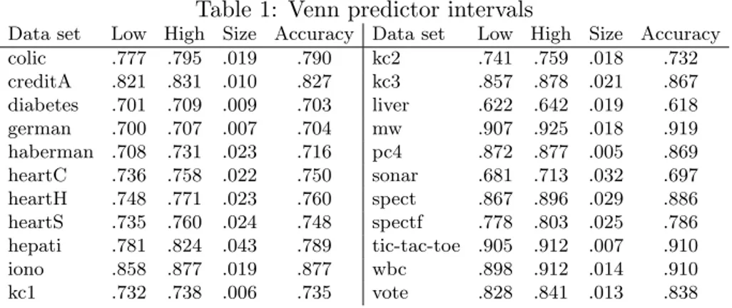
Starting with analyzing the Venn predictors’ probability estimates, Table1below shows the probability intervals, and the actual accuracies on each data set. First of all, we see that the intervals are quite narrow. In fact, the mean interval width, averaged over all data sets, is less than two percentage points. In addition, it is reassuring to see that for an absolute majority of the data sets (18 of 22), the empirical accuracy is also inside the probability intervals.
Table 1: Venn predictor intervals
Data set Low High Size Accuracy Data set Low High Size Accuracy
colic .777 .795 .019 .790 kc2 .741 .759 .018 .732 creditA .821 .831 .010 .827 kc3 .857 .878 .021 .867 diabetes .701 .709 .009 .703 liver .622 .642 .019 .618 german .700 .707 .007 .704 mw .907 .925 .018 .919 haberman .708 .731 .023 .716 pc4 .872 .877 .005 .869 heartC .736 .758 .022 .750 sonar .681 .713 .032 .697 heartH .748 .771 .023 .760 spect .867 .896 .029 .886 heartS .735 .760 .024 .748 spectf .778 .803 .025 .786 hepati .781 .824 .043 .789 tic-tac-toe .905 .912 .007 .910 iono .858 .877 .019 .877 wbc .898 .912 .014 .910 kc1 .732 .738 .006 .735 vote .828 .841 .013 .838
While the fact that the Venn predictors are well-calibrated is no surprise, it must be noted that the intervals produced by the inductive Venn predictor are much smaller than
what is typically the case when using the original transductive approach, see e.g., Pa-padopoulos(2013). This is consistent with the findings in Lambrou et al. (2015), and the reason is quite straightforward; when using the transductive approach, the model is actu-ally re-trained for each new test instance and class, leading to quite unstable models. In the inductive approach, though, the model is both trained and applied to the calibration set only once, i.e., the test instance does not affect the model at all, and only moderately impacts the prediction intervals.
Turning to the overall quality of the estimates, Table 2 below shows the different esti-mates (averaged over all instances for each data set) and the corresponding accuracies.
Table 2: Quality of estimates
Estimates Accuracies Differences
Data set LaP Platt Iso Venn LaP Platt Iso Venn LaP Platt Iso Venn
colic .897 .819 .822 .786 .784 .799 .837 .790 .113 .020 -.015 -.004 creditA .912 .850 .834 .826 .828 .827 .836 .827 .084 .023 -.002 -.001 diabetes .872 .733 .726 .705 .712 .715 .720 .703 .160 .017 .006 .002 german .793 .704 .699 .703 .612 .703 .700 .704 .181 .001 -.001 -.001 haberman .805 .725 .712 .719 .667 .712 .703 .716 .138 .013 .010 .004 heartC .876 .773 .761 .747 .734 .753 .757 .750 .142 .020 .004 -.003 heartH .875 .789 .779 .759 .767 .767 .775 .760 .109 .022 .004 -.001 heartS .877 .773 .761 .747 .759 .753 .756 .748 .118 .019 .004 -.001 hepati .893 .820 .794 .802 .772 .793 .784 .789 .121 .027 .010 .013 iono .941 .889 .867 .867 .880 .879 .884 .877 .061 .010 -.016 -.010 kc1 .858 .737 .740 .735 .683 .735 .736 .735 .176 .002 .004 .000 kc2 .891 .772 .771 .750 .730 .754 .768 .732 .161 .018 .003 .019 kc3 .916 .875 .851 .867 .835 .864 .858 .867 .080 .011 -.007 .000 liver .827 .646 .659 .632 .639 .632 .641 .618 .188 .014 .018 .014 mw .936 .924 .902 .916 .897 .916 .914 .919 .039 .007 -.012 -.003 pc4 .945 .889 .880 .874 .871 .879 .881 .869 .074 .010 -.001 .005 sonar .908 .719 .716 .697 .713 .700 .704 .697 .194 .019 .012 .000 spect .884 .892 .861 .882 .851 .887 .888 .886 .032 .005 -.027 -.005 spectf .911 .800 .785 .790 .742 .787 .785 .786 .169 .013 .000 .005 tic-tac-toe .917 .928 .900 .908 .927 .911 .918 .910 -.010 .017 -.018 -.002 wbc .941 .922 .899 .905 .915 .911 .916 .910 .026 .011 -.017 -.005 vote .886 .863 .839 .834 .843 .840 .845 .838 .043 .023 -.006 -.004 Mean .889 .811 .798 .793 .780 .796 .800 .792 .109 .015 -.002 .001
Starting with the Laplace estimate, we see that it systematically overestimates the true accuracies. In fact, the Laplace estimate is on average more than ten percentage points too optimistic, i.e., it is obviously misleading. In this study, the estimates from Platt scaling are also always larger than the true accuracies. Even if these differences may appear to be rather small in absolute numbers (approximately 1.5 percentage points on average), the fact is that Platt scaling too turned out to be intrinsically optimistic, i.e., misleading. The isotonic regression, on the other hand, appears to be well-calibrated, specifically there is no inherent tendency to overestimate or underestimate the accuracy. This is clearly also true for the Venn predictor; in fact, when looking at each and every data set, the probability estimates are remarkably close to the true accuracies. Even when compared to the successful
isotonic regression, the Venn preditor estimate is actually more precise, on a large majority of the data sets.
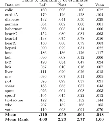
Table 3 below shows the reliability scores for the different techniques. As described above, this is a direct measurement of the quality of the probability estimates, so it should be regarded as the main results of this paper. Here, it must be noted that for reliability, lower values are actually better, contrary to the English language. To enable a direct comparison, the four setups were ranked on each data set, and the last row of Table3shows the mean ranks over all data sets.
Table 3: Reliability of estimates
Data set LaP Platt Iso Venn
colic .160 .096 .100 .072 creditA .179 .126 .128 .104 diabetes .132 .041 .050 .029 german .064 .002 .006 .001 haberman .066 .008 .014 .006 heartC .152 .080 .081 .063 heartH .138 .075 .078 .056 heartS .150 .080 .079 .063 hepati .090 .029 .031 .022 iono .186 .136 .126 .117 kc1 .090 .008 .012 .006 kc2 .120 .034 .047 .024 kc3 .057 .010 .016 .007 liver .111 .020 .026 .015 mw .036 .007 .011 .005 pc4 .076 .029 .037 .021 sonar .183 .055 .057 .043 spect .026 .004 .008 .003 spectf .105 .015 .022 .012 tic-tac-toe .172 .165 .152 .144 wbc .207 .182 .168 .165 vote .119 .093 .091 .070 Mean .119 .059 .061 .048 Mean Rank 4.00 2.23 2.77 1.00
First it should be noted that all three general calibration methods, i.e., Platt scaling, isotonic regression and the Venn predictor improve on the Laplace estimate, thus showing that these kind of techniques may be necessary for converting standard decision trees into well-calibrated PETs. Most importantly, though, we see from the mean rank of 1.00 that the Venn predictor estimate is actually the most reliable on each and every data set. This is, of course, a very strong result, showing that a Venn predictor is not only perfectly calibrated in theory (i.e., in the long run) but also remarkably well-calibrated in practice, even when the data sets are fairly small. Specifically, it is of course very encouraging to see that the Venn predictor clearly outperforms all standard choices. Finally, it is interesting to see that Platt scaling, despite systematically overestimating the accuracy, still is more reliable than the isotonic regression.
In order to determine any statistically significant differences, we used the procedure recommended by Garcıa and Herrera (2008), and performed a Friedman test (Friedman,
1937), followed by Bergmann-Hommel’s dynamic procedure (Bergmann and Hommel,1988) to establish all pairwise differences. From this analysis, we see that all differences are actually significant at α = 0.05, i.e., there is a clear ordering with regard to reliability. 5. Concluding remarks
This paper has presented the first large-scale comparison of Venn predictors to existing tech-niques for calibrating probabilistic predictions. The empirical investigation clearly showed the capabilities of a Venn predictor; the produced prediction intervals were very tight, and the probability estimates extremely well-calibrated. In fact, using the reliability criterion, which directly measures the quality of the probability estimates, the Venn predictor esti-mates were more exact than Platt scaling and isotonic regression on every data set.
Directions for future work include evaluating Venn prediction as a calibration technique also for other learning algorithms, such as random forests, as well as considering more elaborate approaches for constructing the underlying categories, e.g., by means of so-called Venn-ABERS predictors (Vovk and Petej,2012), potentially further strengthening the per-formance of the Venn predictors.
Acknowledgments
This work was supported by the Swedish Knowledge Foundation through the project Data Analytics for Research and Development (20150185).
References
Kevin Bache and Moshe Lichman. UCI machine learning repository, 2013. URL http: //archive.ics.uci.edu/ml.
Beate Bergmann and Gerhard Hommel. Improvements of general multiple test procedures for redundant systems of hypotheses. In Multiple Hypotheses Testing, pages 100–115. Springer, 1988.
H. Bostr¨om. Calibrating random forests. In IEEE International Conference on Machine Learning and Applications, pages 121–126, 2008.
Leo Breiman, Jerome Friedman, Charles J. Stone, and R. A. Olshen. Classification and Regression Trees. Chapman & Hall/CRC, 1984. ISBN 0412048418.
G. Brier. Verification of forecasts expressed in terms of probability. Monthly Weather Review, 78(1):1–3, 1950.
M. Friedman. The use of ranks to avoid the assumption of normality implicit in the analysis of variance. Journal of American Statistical Association, 32:675–701, 1937.
Alexander Gammerman, Volodya Vovk, and Vladimir Vapnik. Learning by transduction. In Proceedings of the Fourteenth conference on Uncertainty in artificial intelligence, pages 148–155. Morgan Kaufmann Publishers Inc., 1998.
Salvador Garcıa and Francisco Herrera. An extension on statistical comparisons of classi-fiers over multiple data sets for all pairwise comparisons. Journal of Machine Learning Research, 9(2677-2694):66, 2008.
Antonis Lambrou, Ilia Nouretdinov, and Harris Papadopoulos. Inductive venn prediction. Annals of Mathematics and Artificial Intelligence, 74(1):181–201, 2015.
Allan H. Murphy. A new vector partition of the probability score. Journal of Applied Meteorology, 12(4):595–600, 1973.
Alexandru Niculescu-Mizil and Rich Caruana. Predicting good probabilities with supervised learning. In Proceedings of the 22nd international conference on Machine learning, pages 625–632. ACM, 2005.
Harris Papadopoulos. Reliable probabilistic classification with neural networks. Neurocom-puting, 107(Supplement C):59 – 68, 2013.
John C. Platt. Probabilistic outputs for support vector machines and comparisons to reg-ularized likelihood methods. In Advances in Large Margin Classifiers, pages 61–74. MIT Press, 1999.
Foster Provost and Pedro Domingos. Tree induction for probability-based ranking. Mach. Learn., 52(3):199–215, 2003.
J. R. Quinlan. C4.5: programs for machine learning. Morgan Kaufmann, 1993. ISBN 1558602380.
Craig Saunders, Alexander Gammerman, and Volodya Vovk. Transduction with confidence and credibility. In Proceedings of the Sixteenth International Joint Conference on Artifi-cial Intelligence (IJCAI’99), volume 2, pages 722–726, 1999.
J. Sayyad Shirabad and T.J. Menzies. The PROMISE Repository of Software Engineering Databases. School of Information Technology and Engineering, University of Ottawa, Canada, 2005. URLhttp://promise.site.uottawa.ca/SERepository.
Vladimir Vovk and Ivan Petej. Venn-abers predictors. arXiv preprint arXiv:1211.0025, 2012.
Vladimir Vovk, Glenn Shafer, and Ilia Nouretdinov. Self-calibrating probability forecasting. In Advances in Neural Information Processing Systems, pages 1133–1140, 2004.
Vladimir Vovk, Alex Gammerman, and Glenn Shafer. Algorithmic Learning in a Random World. Springer-Verlag New York, Inc., 2005.
B. Zadrozny and C. Elkan. Obtaining calibrated probability estimates from decision trees and naive Bayesian classifiers. In Proc. 18th International Conference on Machine Learn-ing, pages 609–616, 2001.