Computation and application of likelihood prediction
with generalized linear and mixed models.
Md Moudud Alam
October 13, 2010.
Abstract
This paper presents the computation of likelihood prediction with the generalized linear and mixed models. The method of likelihood prediction is brie‡y discussed and approximate formulae are provided to make easy computation of the likelihood prediction with generalized linear models. For complicated prediction problems, simulation methods are suggested. An R add-in package is accompanied to carry out the computation of the predictive inference with the generalized linear and mixed models. The likelihood prediction is applied to the prediction of the credit defaults using a real data set. Results show that the predictive likelihood can be a useful tool to predict portfolio credit risk.
Key words: Predictive likelihood, Pro…le predictive likelihood, Coverage inter-val, Future value prediction, Credit risk prediction, R-package.
1
Introduction
In real world application we often want to make prediction. For example, while processing a credit application the credit issuer needs to predict the probability of the borrower being able to repay the loan. However, the computational procedure to produce a predictive inference is rarely available in the existing software. To illustrate the computational issue let us consider the statistical software (R Development Core Team 2009) as an example. R has a generic function, predict(), which is supposed to produce predictive inferences. When it is applied to some object class, e.g. lm, one gets predictive inferential statistics computed. However, the ‘predict’ method is not implemented for all statistical model objects in R. And when it is implemented, it might produce merely a …tted value not a predicted value. Note that …tted value refers to the expected outcome within the observations actually used for the model …tting while the predicted values refer to those for the future observations.
In R, the glm function implements generalized linear models (McCullagh & Nelder 1989) while lme (package: nlme; Pinheiro & Bates (2000)), lmer (package: lme4; Bates
School of Technology and Business Studies, Dalarna University and Swedish Business School, Örebro University. Contact: Dalarna University, SE 781 88 Borlänge, Sweden; maa@du.se .
(2005)) and hglm (package: hglm; Rönnegård, Shen & Alam (2010)., 2010) implement lin-ear and generalized linlin-ear mixed models (GLMM; McCulloch and Slin-earle, 2001). Though, there are predict methods in R for glm and lme, they produce the …tted values, not the predicted values. The predicted values are sometimes but not necessarily the same as the …tted values and the uncertainty is obviously di¤erent (Bjørnstad 1996, Patel 1989). Furthermore, the predict method is not available for lmer and hglm object class (see appendix A.3 for a complete list of predict methods). The unavailability of predictive inference is not particular to R, the lack is similar if one choose an alternative software such as SAS (Littell, Milliken, Stroup & Wol…nger 1996).
The unavailability of computational procedures for prediction may not be attributed to their limited usefulness, rather it is due to the lack of theoretical research and empirical evidences on the precision and the applicability of the predictive inferential framework for the generalized linear and mixed models. In this paper we present computational details of the likelihood prediction for the GLM and GLMM. We propose three di¤erent ways to approximate the computation of the likelihood prediction for GLM and GLMM and compare their performances by Monte-Carlo simulations. We also give an accompanying R add-in package to carry out the predictive inference.
The procedures are illustrated by a standard text book example (Davison & Hinkley 1997, PP. 342–345) on predicting aids reports in England and Wales and an application of the predictive inference using a real data set on credit defaults. Assuming that the credit defaults can be modelled by using a generalize linear mixed models, we compare the performance of the di¤erent strategies to predict future credit risk. By simulation and by application to a real data set on credit defaults we show that the predictive likelihood (Bjørnstad 1990) is a useful tool to predict credit defaults and to compute the uncertainty. It has been shown elsewhere that both the uncertainty in the model parameters and the uncertainty in the future independent variables can be handled in the framework of predictive likelihood. That enables us to make a valid statement of uncertainty about the credit defaults prediction.
The rest of the paper is organized as follows. Section two gives a short introduction to predictive likelihood. Section three describes how the predictive likelihood can be applied to generalized linear models and demonstrates its superiority over the naive frequentist prediction by means of simulation. Section four illustrates the use of pred package to carry out predictive computation for GLM. Section …ve shows the usefulness of likelihood prediction in predicting credit risk using real data sets from two Swedish banks. Section six concludes.
2
Likelihood prediction
Let us denote the observed response with y, future (not observed) response as y ; observed covariate X and unobserved covariate X and the vector of model parameters as = ( 1; 2; :::; p) : Note that we use superscript asteric (e.g. X ) to indicate unobserved part
of an observable quantity (see Alam (2010b) for a detailed description of the notation system). Then the likelihood principle (Berger & Wolpert 1988, Bjørnstad 1990)) states
that all the sample information about ; X and y is contained in the joint likelihood
L (y ; ; X jy; X) = f (y; y ; X jX; ) (1)
Unlike the estimation problem, the inferential interest of the prediction problem centered on y while all other unobservable, both parameters and variables, are nuisance parameters and variables. However, the likelihood principle does not state as to how the information about y should be extracted from the joint likelihood (Berger and Wolpert, 1988). A direct maximization of (1) w.r.t. y ; and X can be disastrous due to the presence of a huge number nuisance quantities (Berger and Wolpert, 1988). Thus some special technique is required to deal with the nuisance parameters and variables in order to extract optimal information on y from the joint likelihood.
The …rst thing one can do is to integrate out the nuisance variables and other random quantities from the joint likelihood. This is justi…ed by the random quantities having a distribution and hence we can integrate them out from the joint distribution to get the marginal distribution of yjX; which is free from the random quantities. It is also noted in the literature that replacing with its observed data maximum likelihood estimator produces misleadingly precise inference on y (Bjørnstad 1996). A survey on the di¤erent ways to produce predictive likelihood inference is presented in (Bjørnstad 1990). Based on an extended de…nition of the likelihood principle (Bjørnstad 1996), …ve out of 14 di¤erent predictive likelihoods surveyed in (Bjørnstad 1990) are found to be proper predictive likelihood. Alam (2010b) pointed out that all the proper predictive likelihoods are not equivalent in general nor can all of them be implemented in every situations. Comparing the theoretical properties and applicability of alternative predictive likelihoods, Alam (2010b) suggested using adjusted pro…le likelihood technique. Let, b be the maximum likelihood estimator (MLE) of based on only observations on and associated with y and b be the MLE based on joint likelihood (based on both observed and unobserved data). Then the adjusted pro…le predictive likelihood is given by
L (y jX) = L zj = b ; X = bX ; y; X I b ; bX
1 2
(2) where I b ; bX is the observed Fisher’s information obtained from the joint log-likelihood. Davison (1986) showed that (2) is the approximate Bayesian posterior predictive density with ‡at prior. A computational implication of the relationship is that we can use exist-ing Markov-Chain Monte-Carlo simulation procedures, e.g. those implemented in Bugs (Spiegenhalter, Thomas, Best & Lunn 2007), to carry out the predictive inference.
3
Predictive inference with generalized linear and
mixed models
Let us assume that the responses, y = fyig (i = 1; 2; :::; n), are independently distributed
as exponential family, given the covariates Xi = (1; X1i; X2i; :::; Xpi)that is f (yijXi; i) =
exphyi ia( )b( i) + c (yi; )
i
parameter: The in‡uence of X’s on y’s are postulated as E (yijXi) = i
g ( i) = i = Xi
The above speci…es a generalized linear model. Incorporating an additional j dimension (cluster) and a random e¤ect, uj; term in above that is writing g ijjuj = i =
Xij +uj where uj v N (0; 2u)we obtain a generalized linear mixed model. The inferential
goal is to produce a set of predictive statistics on the future responses, y = fyig (i =
n + 1; n + 2; :::; n + m), after observing yi; Xi. Denote the observed Xi associate with yi
as _Xi
Assume that the dispersion parameter to be known, which is true only for the Poisson and the binomial family and consider the case of canonical link, for simplicity. The adjusted pro…le likelihood for the GLM is given by
L (y jXF; y) = exp 2 4y T Fb 1Tdiag n b bi o a ( ) + c (yF; ) 3 5 1 a ( )X T FWXF 1 2 (3)
where yF = yT; y T T; bi is the MLE of i based on yF and XF is the design matrix
consisting of X and _X and W is the diagonal weight matrix. A direct maximization of (3) or …nding a normalizing constant to get (3) a density (or mass) function is a challenging task. Especially, for y being discrete, (3) has to be evaluated for every possible combination of y . However, we can apply a simulation based computation to draw random sample of y from the un-normalized density L (y jX) : Its connection to Bayesian posterior density allows us to use Bayesian posterior predictive simulation for y . In absence of any computational method, it can be implemented through Markov-Chain Monte-Carlo techniques. However, using normal approximation to posterior distribution of the parameters we have a …rst approximation method which we refer to as approximate predictive simulation.
3.1
Approximate predictive simulation
We treat (3) as an un-normalized Bayesian posterior predictive distribution with ‡at prior. Since the MLE of is also the posterior mode, we estimate the model parameters using formal likelihood method on the observed data only. Let, ^ be the MLE and I ^ is the information matrix for : Assume that the posterior distribution of is symmetric around ^ and can be approximated by a normal density, the predictive simulation can be carried out in the following way.
1. Draw a random sample on ^ from ^ v N ^; I ^ 2. Draw a random sample on y from y v f y j = ^
This algorithm approximates the Bayesian posterior as long as the normal approxi-mation to the posterior distribution of holds. It also has a frequentist explanation. If were known, then the predictive distribution of y would be f (y j ) : Substituting b for in f (y j ) would produce a naive predictor (Alam 2010) which does not take uncertainty in b into account. Since the b is estimated from the observed data, after correcting for the uncertainty for b, the predictive distribution should be p (y ) =R f y j^ p ^ d^ where the p ^ is the current estimate of uncertainty about the true parameter : Thus the simulation method is simulating draws from p (y ) my treating p ^ as a normal density. Besides the simulation based approach we can also use other approximation method to compute predictive statistics from (3). Using the …rst order Taylor’s approximation to the score function of joint likelihood we obtain our second approximation which is given next.
3.2
First order approximation
In order to obtain an analytical expression for the predictive likelihood (3) we need to know bi where bi = Xib for a GLM with canonical link. Thus we need to know the
analytical expression for b which has a close form expression only for the Gaussian family with identity link. In other cases b is computed through an iterative procedure because analytical expression of b as a function of the observed data is not available. However, the estimate of b is obtained by equating the score function of the joint likelihood, denoted by l , to zero. Hence we obtain b from
@l
@ = 0
Using a …rst order Taylor’s approximation to @l@ around b we obtain @l @ =b+ @2l @ @ T T b 0 ) b b " @2l @ @ T 1 @l @ # =b (4) The exact mathematical expression for @ @@2l T and
@l
@ are well-known for the GLMs (see
e.g. Wand, 2002) and are given, for canonical link, by @2l @ @ T = 1 a ( )X T Fdiagfb00(XF )g XF and @l @ = 1 a ( )X T F (yF b0(Xz ))
Substituting in (4) we obtain b b + XTFdiagnb00 XF^ o XF 1 XTF yF b0 XF^ =^ (5) A similar expression can also be given for the non-canonical links but the second term in the right hand side of (5) becomes more messy in that case1. Substituting b in (3)
we obtain an approximate predictive likelihood for y : The remaining task is either to maximize L (y jX; y) ; if sensible, or to normalize it to make it a probability density (or a mass) function.
For Gaussian GLM with identity link we have
b b + XT FXF 1 XTF yF XFb ) yF XFb = yF XFb XF XTFXF 1 XTF yF XFb ) yF XF^ = I XF XTFXF 1 XTF yF XFb ) yF XF^ T yF XF^ = yFT I XF XTFXF 1 XTF yF Note that yF XFb T
yF XFb determines the predictive likelihood uniquely
for the Gaussian GLM with known dispersion parameter. In order to obtain the exact predictive distribution we make use of the following lemma (Lemma 1) due to Eaton & Sudderth (1998). Lemma 1: Denote SF = yTF I XF XTFXF 1 XT F yF , ^ = XTX 1 XTy where,
X is the design matrix associated with the observed y, _X be the design matrix associated with y and S = y X^ T y X^ then the following identity holds
SF = S + y X^_ T
I+ _X XTX 1X_T
1
y X^_ y
With the help of Lemma 1, we get the predictive density of y for the Gaussian GLM with identity link as
L (y jXF; y)_ exp 1 2a ( ) y X^_ T I+ _X XTX 1X_T 1 y X^_ (6)
that is the predictive distribution of y is multivariate normal with mean _X^ and variance a ( ) I + _X XTX 1X_T which is exactly the same as the one given in Bjørnstad (1996).
Thus the …rst order approximation is exact for the Gaussian GLM with identity link. Note that the mean prediction from L (y jXF; y)is also the BLUP for the above Gaussian case.
The approximation method above and the one in section 3.1 are computationally too extensive since in absence of a general solution for the normalizing constant for L (y jXF; y) we have to rely on Markov-Chain Monte-Carlo techniques. However, if a
point predictor and a measure of uncertainty of the point predictor is concern, we can use the following, third, approximation method.
1Substituting E @2l
@ @ T for @ 2l
3.3
Approximate point prediction
From the GLM theory we know that the maximum likelihood estimation of is equivalent to iteratively solving a weighted least square regression (McCullagh & Nelder 1989). This is computationally equivalent to the ML estimation from a multivariate normal model. Thus, using the normal approximation, the joint likelihood of i = i + (yi i)
@ i
@ i;
i = 1; 2; :::; (n + m)at the ith iteration of the estimation procedure can be expressed as
L ( jXF; yF) = 1 (2 jWj)(n+m)=2exp 1 2( XF ) T W 1( XF ) (7)
where W is the so called diagonal weight matrix such that wii1 = V ( i) @ i
@ i
2
and V ( i)
is the variance function: The normal linear model theory gives us the best linear unbiased predictor (which is also the likelihood predictor) as b = Xb where, b = b is the ML estimator of obtained from the observed data only. But, E (yi i)
@ i
@ i = 0;in turn,
produces the likelihood predictor for y as b
yi bi = g 1 X_ib ; i = n + 1; :::; n + m (8)
This is also a naive predictor. However, we do not use the naive estimate of variance of b
yi which would be V ar (ybi) = a b V (bi). Instead, the variance of byi is calculated in the following way
V ar (by ) = Ey V ar y jb + V ary E y jb
) V ar (by ) = E (V (b ) a ( )) + V ar g 1 X b_
Using the delta method to calculate V ar g 1 X b_ , substituting V (b ) a b for
E (V (b ) a ( )) we obtain the sample estimate of the standard error (SE) of by as
b se (ybi) s V (bi) a b + a b @ i @ i 2 j i=bi _ Xi(XTWX) 1X_T i (9)
From (6) we note that (8) and (9) provides the exact mean prediction and predictive standard deviation for the Gaussian model with identity link. For binomial response, (9) simpli…es into b se (byi) = q bi (1 bi) + (bi (1 bi)) 2 _ Xi(XTWX) 1X_iT
where the …rst term in the se (b byi) is well-recognized as the binomial variance and the second term being the additional uncertainty due to the estimation of .
In matter of fact, the estimation of GLMM is also carried out in penalized quasi likelihood (Breslow & Clayton 1993, PQL) or pseudo likelihood (Wol…nger & O’Connell 1993) where an iterative weighted least square regression on the modi…ed response is
used to get an updated estimate for :Thus, treating the variance components as known, the same approximation for GLM can be extended to produce the predicted values for yi i.e. ybi = g 1(bi). This works under the assumption that the variance components are known which is often not the case. Therefore, we recommend using simulation based prediction for GLMM.
4
Monte-Carlo study
In order to compare the performance of the naive predictor (NP), Likelihood predictor (LP) and several approximations to LP we conduct a small simulation experiment with a logistic GLM. We generate 60 observations from a binomial (1; i) distribution where,
log i
1 i = i; i = 1; 2; :::; 60 and i = Xi . The …rst column of the design matrix, X;
is 1 and the rests are independent simulated draws from N5(0; diagf0:7; 0:5; 1; 0:8; 1:2g).
The model parameters are arbitrarily chosen as = ( :6; :2; 1:1; 0:7; 0:8) : With the …rst 40, out of the 60, observations we …t a logistic model and estimate b with the maximum likelihood method. Consequently the naive predictoryei for yi, i = 41; 42; :::; 60
is given by eyi = _Xib: The LP byi for yi is given by solving (3). Since the parameter
space for y is discrete, in principle, we have to evaluate the L (y jX) over all the 220
possible combination of y which requires a tremendous computational work. However, L (y jX) is approximately equivalent to Bayesian posterior predictive density with ‡at prior. Therefore, we use Bayesian posterior simulation with MCMC to compute ybi: We implement the Bayesian computation of the logistic model with ‡at prior via MCMClogit function of MCMCpack library (Martin & Quinn 2006) in R and summarize the predictive density with 4000 MCMC samples. We replicate the whole experiment 1000 times and summarize the results with the following statistics; the average percentage of correct prediction and the average absolute error per unit of standard error. We also use the approximate standard error given in (9) to compute the absolute error per unit of standard error.
In terms of the percentage of correct prediction both the methods, NP and LP are similar. However, in terms of absolute error per unit of SE, LP outperforms the others though the di¤erence in very slim. A comparison of their empirical cumulative distribution is given in Figure 1.
0 1 2 3 4 5 0.0 0.2 0.4 0.6 0.8 1.0 abs(error)/SE C um. P ro b. LP(Apprx.) LP(MCMC) NP
Figure 1: Simulated cumulative densities of the absulute error per unit of SE for LP, Approximate LP and NP.
Figure 1 presents the empirical cumulative densities of the average absolute error per unit of standard error. The thick solid line represents approximate likelihood method with SE calculated by using (9), the broken line presents likelihood prediction using Bayesian method implemented through MCMC and the solid thin line represents Naive prediction. They do not look very di¤erent from each other with LP(MCMC) being the best in terms of its range. However, the ‡at tail of NP and LP approximation can be explained from their inability to handle extreme predicted values. Therefore, we conclude that as long as the predicted values are not very extreme, the NP along with its standard error calculated from (9) can be used. In other special cases, the simulation method is to be preferred.
5
Use package pred for computation
This paper accompanies with an R add-in package, pred, to facilitate the computation of the predictive inference. Currently the package only covers the prediction methods discussed above. In the following we present some examples of producing likelihood prediction using the package: pred.
As a demonstrative example, we use the aids data set from Davison & Hinkley (1997). The data set contains information on the number of AIDS reports in England and Wales between the second quarter of 1983 and the fourth quarter of 1992. The observations are cross classi…ed according to the diagnostic period and reporting delay, in three months interval. The AIDS cases are not all reported immediately after the diagnosis. Sometimes, it takes as long as 14 quarters from the diagnosis before some AIDS cases are reported. The data set is also available in boot library. The problem is to predict the number of AIDS reports at previous and current quarters while the prediction takes place at the 4th
We …t a Poisson model for count response, number of AIDS reports. Based on the …tted model we can calculate predicted values in R in the following way.
>library(boot) >data(aids)
>g1<-glm(y~factor(delay)+factor(year):factor(quarter),
+family=poisson,data=aids[aids$dud==0,]) ## dud=0 indicates complete data >predict(g1,newdata=aids[aids$dud==1]) 375 389 390 403 404 ... 1.650853590 0.603278659 1.576317870 -0.074387547 0.793893031 ... ... 566 567 568 569 570 ... 1.584843220 1.310625193 0.334686204 1.202966781 2.176005992 Warning message:
In predict.lm(object, newdata, se.fit, scale = 1, type = ifelse(type == : prediction from a rank-deficient fit may be misleading
Above we note that R produces the …tted values as the predicted value and that it does not produce any measure of prediction uncertainty. To work out those with the pred library we do the following
>library(pred) >pred(g1,newdata=aids[aids$dud==1]),se.pred=T) 375 389 390 403 404 ... 1.650853590 0.603278659 1.576317870 -0.074387547 0.793893031 ... ... 566 567 568 569 570 ... 1.584843220 1.310625193 0.334686204 1.202966781 2.176005992 Standard error of the predicted values
375 389 390 403 404 ...
2.802649e+01 1.941082e+00 1.947709e+01 1.262302e+00 2.516129e+00 ...
... 566 567 568 569 570
... 2.651991e+01 9.370777e+00 1.815760e+00 7.168442e+00 1.255263e+03 Note that the default prediction method for pred is the approximate point prediction (Sec-tion 3.3) which can be speci…ed through an argument method="PtP" in the pred func(Sec-tion. Currently, "PtP" and the approximate predictive simulation (Section 3.1; "SLP1") are the two available options for the method argument to work with the glm object class. Getting the point prediction for each of the missing values was not the aim of the data analysis, rather we want to predict the total number of AIDS patients in a particular quarter within the years 1990–1992. We demonstrate how that can be obtained by making prediction for the 4th quarter of 1992.
>p1<-pred(g1,newdata=aids[aids$dud==1]),method="SLP1",nsim=10000) >s1<-p1$predsim ### Simulated prediction, one clumn for wach obsn. >s<-apply(s1[,92:105],1,sum)
> 67+quantile(s,c(.025,.975))
2.5% 97.5%
>67+median(s) [1] 437
> 67+mean(s) [1] 600.3048
Hence, we get a 95% prediction interval (137, 2038) for the fourth quarter of 1992 which is much wider than the bootstrap prediction interval (357, 537) reported in Davison and Hinkley (1997). The huge length of the likelihood prediction interval can be explained from the fact that in quarter 4 of 1992 we only have report (67 infection) of the current quarter while prediction is based on what would have been reported in the next 14 quarters. In matter of fact there were about 2597 AIDS reports in England and Wales in 1992 (AIDS/HIV Quarterly Surveillence Tables 2003). Thus a mean prediction of 600 AIDS reports for quarter 4 in 1992 sounds reasonable.
6
Prediction of portfolio credit defaults
In order to make a sound prediction of portfolio credit risk and the value at risk we need a good statistical model as well as a sound predictive technique. The modeling issues are even challenging and the credit risk model often turns out to be very complicated. A huge amount of work on them are available in the literature (see e.g. Hao, Alam & Carling (2010) for a review). Taking the modeling framework presented in Alam (2010a) we demonstrate how to predict the future credit risk in a statistically sound way.
Let yiktdenote the state of default (1 = default, 0=non-default) of loan i (i = 1; 2; :::; nkt)
in industry k (k = 1; 2; :::; K) and at time t (t = 1; 2; :::; T ) : Following the framework of GLMM, the conditional probability of default, pitk = E (yiktjukt) ; is modelled as
yiktjuktv Bin (1; pikt) and
g (pikt) = Xikt + Ziktut (10)
where g (:) is called the link function and g (pikt) = log 1+ppikt
ikt gives a logistic mixed
models which is also used in McNeil and Wendin. We use the logistic link in this paper. The use of g (pikt) = log ( log (1 pikt))gives a complementary log-log model (as used in
Carling, Rönnegård & Roszbach (2004)) and g (pikt) = 1(pikt)produces a probit mixed
model. Xikt is a row vector of loan, industry and time speci…c covariates where each
column of it corresponds to a covariate, is a column vector of …xed e¤ects parameters, Zikt is the iktth row of the design matrix associated with the random (unobservable)
e¤ects ut = (u1t; u2t; :::; uKt)T and ut’s are iid random variables having some speci…c
distribution, f (u) : Conventionally, the random e¤ects vector, u; is assumed to have a multivariate normal distribution with a 0 mean vector and a covariance matrix, D, i.e. f (u) = jDj
1 2
(2 )K2
exp 12uTD 1u . It was found in Alam (2010a) that the dependence in u t
over time, t; is not signi…cant:
After the model parameters have been estimated a naive prediction (NP) of credit defaults of ikth loan at time t0 > T would be given as
where Xikt is the row vector of the covariates observed at time t: After observing Xikt
it makes sense to model yikt conditional on Xikt. But in this case we do not observe all
the future covariates Xikt0 at time t0. There are some covariates which e.g. macro indices
(output gap, slope of the yield curve), …rm speci…c characteristics such as, future sales, future asset values etc. can only be observed at time t0. Therefore, we also examine the
e¤ect of stochastic future covariates on the prediction performance.
6.1
Data description
We use the data set of Carling et al. (2004) to demonstrate the usefulness of the predictive likelihood in credit defaults prediction. The data set contains information on the credit history of 100,926 small and medium size aktiebolag, the approximate Swedish equivalent of US corporations and UK limited companies, from two major Swedish banks between the 2nd quarter of 1994 and the 2nd quarter of 2000. Besides the bank data on credit status, the data set contains information on accounting variables of the borrower companies e.g sales, assets, liabilities etc., di¤erent remarks of the credit bureau and two macro variables being the slope of the yield curve and the output gap. We use the …rst 23 quarters’data to build our model and the rest two quarters to evaluate the performance of the likelihood prediction compared to a naive frequentist’s prediction. This simulates a situation as to what would have happened if we were to predict credit defaults for two quarters ahead based on the information up to the 4th quarter of 1999.
There are 6 clusters (industries) which are de…ned by merging the SNI industries (see www.scb.se) at the …rst two digits level, in a way that closely resembles the industry de…nition of Carling et al. (2004). We consider the credit defaults to be correlated both within and between clusters but not over time, as proposed in Alam (2010a). The mean part of the model is the same as in Carling et al. (2004) but we use a logit link whereas a complementary log-log link was used in Carling et. al (2004).
6.2
Data analysis and results
We …t the GLMM given in (10). In the implementation, we …t the GLMM with ukt
N (0; diag ( 2
k)) : Later, we use the random e¤ects obtained from the …tted model to
estimate D i.e. we use
b D= 1 T T X t=1 utuTt
where, ut = (bu1t;bu2t; :::;buKt)T is the vector of realized random e¤ects for time t. The
applicability of the above method was examined in (Alam & Carling 2008). In addition, we also …t a simple GLM having the same …xed e¤ects as in (10) but the random e¤ects are dropped.
In order to compare the performance of the GLMM and the GLM model in credit risk prediction, we use a simulation based prediction from the two models. We …t both of the models using the data up to quarter 23. Then we use them for predicting the credit defaults for quarter 24 and 25. Finally we compare the model implied defaults probability and the loss given defaults (LGD) de…ned as LGD = EAD P (Def ault) where EAD is
the exposure (outstanding loan) at default with its real …gures at the respective quarters. In simulation, we use the normal approximation method described in Section 3.1. For GLMM, we generate from N b; I where b and I are the model estimated …xed e¤ects and their respective observed information matrix. The random e¤ects,ut’s, are
simulated from N 0; bD :The predicted response is simulated, given the parameters and the covariates available at quarter 23 using a binomial model with mean ikt= g 1( ikt)
where g is the logistic link function.
Table 1 Comparison between GLM and GLMM in credit defaults prediction Probability of default (%) Loss given default (% of total credit)
Quarter Observed GLM GLMM Observed GLM GLMM
24 0.31 0.25 0.27 0.16 0.11 0.13 (0.20, 0.29) (0.1, 0.48) (0.01, 0.12) (0.06, 0.24) 25 0.72 0.16 0.22 2.41 0.08 0.11 (0.11, 0.21) (0.1, 0.38) (0.07, 0.11) (0.05,0.20) 24 & 25 0.44 0.22 0.26 0.97 0.10 0.13 (0.18, 0.26) (0.15, 0.40) (0.09, 0.11) (0.07, 0.20)
Note: Values in the parenthesis represent 95% quantile interval
Table 1 presents the observed and the model implied probability of defaults and the loss given defaults per unit of outstanding total credits during the quarters 24 and 25. In application, to get the quarterly breakdown for quarter 24 and 25 by using all the time dependent variables …xed at quarter 23 while the time independent variables e.g. credit bureau remarks, credit duration are taken from the records at quarter 24 and 25 since they would be known at quarter 23. Therefore we see that the prediction model uses only the loans that were in the data base at quarter 23 and at least one of the other two quartets, 24 and 25. The observed proportion of defaults and the loss given default are calculated on the basis of all the loans which were actually available in the particular quarter.
Table 1 reveals that neither of the model performs very well, in terms of mean defaults prediction. For example at quarter 24, the observed proportion of defaults was 0.31% while the proportion was predicted as 0.25% by GLM and 0.27% by GLMM. A striking feature of GLM is that it produces the quantile interval misleadingly tight while the GLMM produces a wider quantile interval due to the consideration of the additional industry shocks (random e¤ects). The 95% quantile interval of the GLMM almost captured the true proportion of defaults at quarter 24 but GLM did not. However, in quarter 25 both of the model failed by a big margin. In matter of fact, quarter 25 is an abnormal quarter in the historical credit risk data in that it has the highest proportion of default among the preceding 10 quarters. The overall proportion of defaults was only 0.55% during the whole 25 quarters while it was 0.19% in quarter 23 and 0.72% in quarter 25. Thus we conclude that none of the models are very successful to capture any abnormal sudden shock which might take place in the future two quarters.
A major drawback of both of the above model is that they consider all the covariates for quarter 24 and 25 as known at quarter 23 which is unrealistic. Though the accounting
variables may be treated as the same, since they are reported only once a year, the macro variables, output gaps and the slope of the yield curve are reported quarterly. The speci…c drawback of the GLMM is that it considers D as known while it uses an estimated D for prediction. Hence, an adjustment for the uncertainty in D is to be incorporated in the predictive simulation.
Since an estimate of the standard error of D is not readily available we use the Bayesian MCMC method to simulate D from its posterior distribution. In the application, we carry out the MCMC simulation in OpenBugs 3.0.2 (Spiegenhalter et al. 2007). It was however found that the Bugs software is very slow with full data set. Therefore, we use a subset of the data containing all the defaults and only a sample of equal number of non-defaults to get the posterior simulation from the GLMM model. We also use weakly informative prior, in stead of ‡at prior for the stability of the simulation. A detailed description of the Bayesian model is given in Alam (2010a).
We model the time series data on yield and output gap using an AR(2) and an AR(4) model and use the respective simulated forecasted values for quarter 24 and 25 for the predictive simulation of defaults probability and LGD. A time series plot of the output gap and the slope of yield curve along with their sample autocorrelation and sample partial autocorrelation plots are given in the appendix. The AIC suggests AR of order 2 for the slope of the yield curve and 7 for the output gap. However, to keep the model reasonably simple, from visual inspection of the time series properties of the above variables (see Appendix) we choose the lag orders 2 and 4, respectively. The simulated probability of defaults and the loss given defaults produced by GLMM after incorporating the additional uncertainties due to the macro variables (TS. forcast) and in D (D and TS) are given in Table 2.
Table 2 Performance of GLMM after incorporating uncertainties in D and time series Probability of default (%) Loss given default (% of total credit) Quarter Observed TS. forecast D and TS Observed TS. forecast D and TS
24 0.31 0.26 0.25 0.16 0.12 0.12 (0.10, 0.50) (0.08, 0.52) (0.04, 0.26) (0.04, 0.26) 25 0.70 0.20 0.20 2.41 0.11 0.11 (0.07, 0.42) (0.06, 0.45) (0.04, 0.23) (0.03, 0.25) 24 & 25 0.44 0.24 0.23 0.97 0.12 0.12 (0.11, 0.43) (0.10, 0.45) (0.05, 0.22) (0.04, 0.23)
Note: Values in the parenthesis represent 95% quantile interval
Table 2 shows that after correcting for the uncertainties involved with the future values of the macro variables and with the estimation of the covariance matrix, D, the mean of the predicted proportion of defaults and loss given defaults do not change a lot but the prediction interval gets wider. For example, for combined credits history data on quarter 24 and 25, the GLMM predicted probability of defaults, before the correction, was 0.26% (see Table 1). After correcting for the macro variables’uncertainty it becomes 0.24% (Table 2, 5th row and 3rd column) and after correcting for the uncertainties in
both for the macro variables and in D it becomes 0.23% (Table 2, column "D and TS", row 5). The model generated 95% prediction interval (0.10, 0.45) now covers the actual
proportion of defaults observed in quarters 24 and 25 together (0.44%). However, the prediction interval for the loss given defaults, once again, fails to capture the abnormality of quarter 25.
7
Concluding discussion
Besides the likelihood prediction, there are other frequentist suggestion for prediction with linear and generalized linear mixed models. A major draw-back of those methods are that they should be assesses case by case and computation procedures are substantially di¤erent between di¤erent classes of models. However, the likelihood prediction o¤ers a uni…ed principle and method for making predictive inference in any situation.
The likelihood prediction may turn out to be computationally challenging but the simulation based methods can be applied in those cases. Applying the approximate pre-dictive simulation for AIDS data and MCMC methods in predicting credit defaults risk we show that likelihood prediction may be useful in predicting future events with GLM and GLMM.
References
AIDS/HIV Quarterly Surveillence Tables (2003), Cumulative uk data to end june 2003, health protection agency (HIV/STI division, communicable disease surveillance cen-tre) and the scottish centre for infection & environmental health, no. 59: 03/2 july 2003. last accessed: October 13, 2010.
URL: http://www.hpa.org.uk/web/HPAwebFile/HPAweb_C/1194947383253
Alam, M. M. (2010a), Industry shocks and empirical evidences on defaults comovements. Unpublished manuscript, Dalarna University.
Alam, M. M. (2010b), Prediction with generalized linear and mixed models under covariate uncertainty, Unpublished manuscript, Dalarna University.
Alam, M. M. & Carling, K. (2008), ‘Computationally feasible estimation of the covariance structure of the generalized linear mixed models (GLMM)’, Journal of Statistical Computation and Simulation 78(12), 1227–1237.
Bates, D. (2005), ‘Fitting linear mixed models in R using the lme4 package’, R News 5(1), 27–30.
Berger, J. O. & Wolpert, R. L. (1988), The likelihood principle, in ‘The IMS Lecture Notes-monograph Series’, Vol. 6, IMS, Hayward.
Bjørnstad, J. F. (1990), ‘Predictive likelihood: a review (with discussion)’, Statistical Science 5(1), 242–256.
Bjørnstad, J. F. (1996), ‘On the generalization of the likelihood function and the likelihood principle’, Journal of the American Statistical Association 91(434), 791–806.
Breslow, N. E. & Clayton, D. G. (1993), ‘Approximate inference in generalized linear mixed models’, Journal of the American Statistical Association 88, 9–25.
Carling, K., Rönnegård, L. & Roszbach, K. (2004), Is …rm interdependence within in-dustries important for portfolio credit risk?, Working Paper Series 168, Sveriges Riksbank.
Davison, A. C. (1986), ‘Approximate predictive likelihood’, Biometrika 73(2), 323–332. Davison, A. C. & Hinkley, D. V. (1997), Bootstrap Methods and their Applications,
Cam-bridge University Press, New York.
Eaton, M. L. & Sudderth, W. D. (1998), ‘A new predictive distribution for normal multi-variate linear models’, Sankhya: The Indian Journal of Statistics (Series A) 60, 363– 382.
Hao, C., Alam, M. & Carling, K. (2010), ‘Review of the literature on credit risk modeling: development of the past 10 years’, Banks and Bank Systems (to appear).
Littell, R. C., Milliken, G. A., Stroup, W. W. & Wol…nger, R. D. (1996), The sas system for mixed models. SAS Inst. Inc.,Cary, North Carolina.
Martin, A. D. & Quinn, K. M. (2006), ‘Applied Bayesian inference in R using MCMCpack’, R News 6(1), 2–7.
McCullagh, P. & Nelder, J. A. (1989), Generalized Linear Models, Chapman and Hall, London.
Patel, J. K. (1989), ‘Prediction intervals: a review’, Communications in Statistics: Theory and Methods 18(7), 2393–2465.
Pinheiro, J. C. & Bates, D. M. (2000), Mixed E¤ects Models in S and S-plus, Springer, New York.
R Development Core Team (2009), R: A language and environment for statistical com-puting. R Foundation for Statistical Comcom-puting.
URL: http://www.R-project.org
Rönnegård, L., Shen, X. & Alam, M. (2010), ‘hglm: a package for …tting hierarchical generalized linear models’, R Journal (to appear).
Spiegenhalter, D., Thomas, A., Best, N. & Lunn, D. (2007), Openbugs user manual (version 3.0.2). last accessed: June 09, 2010.
URL: http://mathstat.helsinki.…/openbugs/Manuals/Manual.html
Wol…nger, R. & O’Connell, M. (1993), ‘Generalized linear mixed models: a pseudo-likelihood approach’, Journal of Statistical Computation and Simulation 48, 233–243.
A
Appendix: Time series properties of the macro
variables
-8 -6 -4 -2 0 2 4 1970 1975 1980 1985 1990 1995 2000 Outputgap YieldFig. A. 1 Plot of the time series data on output gap and the slope of the yield curve.
0 5 10 15 20 -0 .2 0 .2 0 .6 1 .0 Lag A CF Outputgap 5 10 15 20 -0 .2 0 .2 0 .6 1 .0 Lag P ar ti al AC F Outputgap
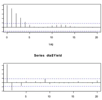
0 5 10 15 20 -0 .2 0 .2 0 .6 1 .0 Lag A CF Series dta$Yield 5 10 15 20 -0 .4 0 .0 0 .4 0 .8 Lag P ar ti al AC F Series dta$Yield
Fig. A. 3 Sample aotocorrelation and partial autocorrelation plot of the solpe of the yield curve.
A.1
Summary of the …tted time series models
Mean AR Parameters Variance
Time Series parameter Lag 1 Lag 2 Lag 3 Lag 4 Parameter
Output Gap -1.13 0.92 0.40 -0.12 -0.25 0.89
(0.05) (0.09) (0.13) (0.12) (0.09)
Slope of Yield Curve 0.58 1.17 -0.37 - - 0.29
(0.09) (0.08) (0.08) -
-Note: Values within parentheses present standard error
A.2
Summary of the time series model forecast
Quarter 24 Quarter 25
Time Series Observed Predicted Observed Predicted
Output Gap 0.14 0.80 0.56 1.03
(0.54) (0.73)
Slope of Yield Curve 1.23 1.03 1.17 0.91
(0.94) (1.45)
Note: Values within parentheses present standard error
A.3
Available methods for predict function in R
The R function methods(generic="name")returns the list of the available methods asso-ciated with any generic function. Including the packages MASS, lme4, nlme and ghlm we obtain the following list of methods for the generic function predict in R.
> library(MASS) > library(nlme) > library(lme4) > library(hglm) > methods("predict") [1] predict.ar* predict.Arima* [3] predict.arima0* predict.glm [5] predict.glmmPQL* predict.gls* [7] predict.gnls* predict.HoltWinters* [9] predict.lda* predict.lm [11] predict.lme* predict.lmList* [13] predict.loess* predict.lqs* [15] predict.mca* predict.mlm [17] predict.nlme* predict.nls* [19] predict.polr* predict.poly [21] predict.ppr* predict.prcomp* [23] predict.princomp* predict.qda* [25] predict.rlm* predict.smooth.spline* [27] predict.smooth.spline.fit* predict.StructTS* Non-visible functions are asterisked