Classification Performance Between Machine Learning and Traditional Programming in Java

(1)

Degree Project, 15 credits

for the degree of Bachelor of Science in Computer Science

Spring Semester 2019

Faculty of Natural Sciences

Classification Performance

Between Machine Learning and Traditional

Programming in Java

(2)

Authors

Abdulrahman Alassadi, Tadas Ivanauskas

Title

Classification performance between machine learning and traditional programming in Java

Supervisor

Kamilla Klonowska

Examiner

Niklas Gador

Abstract

This study proposes a performance comparison between two Java applications with two different programming approaches, machine learning, and traditional programming. A case where both machine learning and traditional programming can be applied is a classification problem with numeric values. The data is heart disease dataset since heart disease is the leading cause of death in the USA. Performance analysis of both applications is carried to state the differences in four main points; the development time for each application, code complexity, and time complexity of the implemented algorithms, the classification accuracy results, and the resource consumption of each application. The machine learning Java application is built with the help of WEKA library and using its NaiveBayes class to build the model and evaluate its accuracy. While the traditional programming Java application is built with the help of a cardiologist as an expert in the field of the problem to identify the injury indications values. The findings of this study are that the traditional programming application scored better performance results in development time, code complexity, and resource consumption. It scored a classification accuracy of 80.2% while the Naive Bayes algorithms in the machine learning application scored an accuracy of 85.51% but on the expense of high resource consumption and execution time.

Keywords

Classification Performance, Algorithms, Java, Benchmarking, Machine Learning, Naïve Bayes, Heart Disease, Supervised Learning, WEKA.

(3)

1. Introduction

1.1 Background

Traditional programming (TP) and machine learning (ML) both aim to solve a problem, where the main difference is in the execution. Machine learning takes the data-driven approach, while the traditional programming approach is heavily dependent on developers' ingenuity to create an algorithm that solves the problem.

A traditional program is a set of instructions to perform a task, it takes the input, performs computations based on the algorithm that was created by the developer and produces the output, where the developer is responsible for the correctness of each possible case that the algorithm may encounter or aim to solve. It cannot evolve without explicitly adding new instructions to adapt to additional scenarios or to produce more precise results [fig 1, left diagram].

Figure 1 - Traditional programming and Machine Learning paradigms. [1]

On the other hand, machine learning programs are implemented by developers and data scientists where they use existing algorithms or write their own based on data that should be trained to create models. These models are then used as the algorithms to accomplish the tasks and produce output for new input data.

Machine learning (ML) gave a machine the ability to learn, where the input for a machine learning program is the input data and the desired output, and letting the machine learns so it can decide the result from a future input. That was a changing point in classification problems, with the help of machine learning algorithms, a program can classify and cluster data after training [fig 1, right diagram].

(6)

6

The process of developing ML programs is more iterative than traditional software development since ML is applied to problems that are too complex for developers to create an algorithm solving it. ML developers and data scientists, therefore, have to experiment more and be ready to test multiple ML algorithms before finding the best one. An application that learns from data can solve many problems that traditional programs cannot, especially when the algorithm to a solution is unknown or too complicated to be hard-coded. There are many examples of the superiority of machine learning applications to non-machine learning ones, like speech and image recognition, that if developers wants to create a voice recognition software in the TP approach, they needs to distinguish the difference between letters in code by specifying the tone pitch of each letter. For the traditional programming it would be possible to create a program that can detect a small set of words that are pronounced by a small group of people having the exact accent, but when the application should interpret millions of words that are being spoken by different groups of people with different accents, surrounding noise or multiple language support, that would be impossible.

1.2 Aim and Purpose

Machine learning as a concept has been around for decades, however, due to the lack of computational power it was not possible to implement at that time. Nowadays technology has advanced and allowed it to become the latest trend in technology. This is due to the huge advantage machine learning has over traditional programs in some areas like e.g. voice and image recognition, spam filtering, disease detection, and many others. However, there are few problems that both traditional programming and machine learning can solve, which raises a question, which one is better in this case?

The purpose of this project is to address the differences in development time, code and time complexity, computation resources, and the results’ accuracy between a traditional program and a machine learning program where both are developed in Java language to classify a set of data when the classifiers are known to the developer.

The authors of the thesis assume that the reader is familiar with programming and Java programming language.

(7)

7

1.3 Research Question

Is the machine learning approach more efficient than traditional programming in a classification problem considering development time, code and time complexity, classification accuracy, and CPU and memory usage?

1.4 Method

This study employs two different research methods. The literature study focuses on the theoretical aspects where it investigates machine learning and its types and algorithms. Heart disease is chosen as a case study; therefore, a literature study also investigates heart diseases and what are the most common causes and risk factors, this information is included in the appendix found in chapter 10. Related work is discussed, and it includes previous studies about detecting heart disease with the help of machine learning. Machine learning algorithms are discussed and performance results from previous studies are presented of different machine learning algorithms in terms of accuracy. To compare the accuracy and maintain focus, heart disease detection is chosen as a case study. The second method employed in this study is an experiment. Chapter 4 introduces tools selected for the study, dataset and implementation of the program. In addition, an interview with a cardiologist through a third-party is carried to exchange questions and answers between the developers and the cardiologist, and to use the information gained from this interview to build the traditional programming application, found in subchapter 4.5, and the full interview questions and answer found in the appendix (chapter 10).

1.5 Limitations

This study does not explain machine learning in detail and does not provide detailed information about machine learning algorithms other than the Naive Bayes, as it is beyond the scope of this study. While there are multiple types of ML, like unsupervised, semi-supervised and reinforcement learning, this thesis will focus on semi-supervised learning since the Naive Bayes classification algorithm is a part of this category.

The datasets found were particularly small, one with 303 for training and 270 instances one for testing.

(8)

8

1.6 Thesis Structure

This thesis employs two methods, a literature study, and an experiment. The literature study investigates what is machine learning, what types of machine learning exist and where it is used to find the most suitable approach for the experiment. Later literature study is conducted to discuss traditional programming and Java programming language. As a case study, heart disease classification is chosen, therefore, the study was conducted to find what are the risk factors and the most common causes of heart disease. Tools to measure the performance of Java programs are introduced and discussed. Lastly, in this chapter, the Naive Bayes algorithm is introduced. Related work from literature study found in chapter 3, introduces work related to classifying heart disease using machine learning.

The experiment part (chapter 4) explains how the experiment was conducted and explains the code that was written and the tools to complete the experiment. WEKA is discussed since it is a key tool essential for the experiment. Then results are presented and evaluated in chapter 5, additional results’ analysis is presented in chapter 6, a discussion about the findings and ethical issues and sustainability are presented in chapter 7, and the conclusion and future work in chapter 8. Finally, the bibliography and the appendix are presented in chapter 9 and 10 correspondingly.

(9)

9

2. Literature Study

2.1 Machine Learning (ML)

ML is a subset of the field of artificial intelligence (AI) that “focuses on teaching computers how to learn without the need to be programmed for specific tasks,” [2]. An algorithm that is trained for detecting disease, can be trained with a different dataset and be used for different tasks.

Exposing huge amounts of data to machine learning techniques can assist in discovering patterns and similarities in the data, where it would be possible to classify and cluster, and ultimately, predict the class value of new input. Machine learning has many types and can be categorized based on its interaction with the data, and the training method whether it was under human supervision or not, or if it learns from a batch of data or gradually from a stream of data.

2.2 Supervised Learning and Classification

Supervised Learning is when the training data flowing to the algorithm is mapped with a label or the desired output, and it is usually a classification task. Furthermore, many supervised classification techniques were developed based on artificial intelligence or statistics.

A classification problem can be defined as follows: “Given a set of training data points along with associated training labels, determine the class label for an unlabeled instance” [3]. In general, a classification algorithm has two phases, the training phase, and the testing phase. The training phase is where the algorithm builds a model from the given data while the testing phase is where the model predicts the label of a data instance, compares it to the given class value and then calculates the accuracy based on the percentage of the right predictions to the total number of instances.

Since the classification problem divides test instances based on their labels into groups, while clustering does the same thing, it is important to distinguish the key difference between classification and clustering, and the reason why classification is supervised, and clustering is unsupervised. Clustering problem divides test instances based on the resemblance among identifiers and without inspecting the relations between identifiers, while classification does a deep analysis to understand the structure of the class and the

(10)

10

relations between identifiers that led to determining a label, furthermore, class labels hold an important property that defines a class and it gives the application a specific task purpose because of the unique nature of the relations between identifiers in a dataset. Real-world (raw) data is often inconsistent, incomplete, unstructured, and may contain errors. Classification algorithms cannot be useful on raw data before preprocessing it, which is done by features selection, labeling the data, filling in the missing values, and eliminating the noise in data.

Noisy data contains invalid or impossible values that affect the structure of the model that will later compromise the accuracy in the testing phase because of overfitting. In addition, feature selection is important to prevent poor modeling which is caused by features being selected by people who are not related to the field where the data is coming from, and they do not know if a feature is related to the desired result.

There are numerous algorithms for supervised learning available for public use and not even one can perform best on all supervised learning problems, based on No Free Lunch theorem [4], each algorithm has its own strengths and weaknesses. An example of popular algorithms in supervised learning is probabilistic classifiers such as Naive Bayes, non-probabilistic binary linear classifiers such as Support Vector Machines (SVM), and Artificial Neural Network (ANN).

2.3 Traditional Programming

Software developers and engineers develop programs that could solve and manage difficult tasks like nuclear reactors control or flight control software. Traditional programming is a powerful tool but requires a solid understanding of the problem that is being solved. To develop the program, developers should identify the problem, determine inputs that are required and develop an algorithm that can solve the problem and would produce the desired output. The algorithms must address all possible cases in the input data to prevent unexpected behavior of the program. Extreme cases of input data have to be tested. Developers have to fully understand how to solve the problem and what is important in solving it. This means that there are limited cases of input and output data for any given algorithm.

Input data is very restrictive and must follow determined standards. Programs developed using this model are not flexible in the sense that if the number of attributes in input data

(11)

11

has changed, the program has to be changed and tested again with the new input data. Additionally, it is difficult to scale an algorithm that is written in traditional programming to handle additional attributes because each possible value of an additional attribute has to be tested for extreme cases and its interaction and relation to other attributes. The number of attributes in input data can be in hundreds or even thousands.

It is difficult and impractical to work with such large data structures in traditional programming like hash tables or that can hold data as large as the Java heap memory size. Developing an algorithm that accommodates a very large number of attributes takes a lot of time for developers, can increase execution time as well as the costs of maintaining and developing the software.

Machine learning introduces a paradigm shift in how we approach these challenging problems. It employs an algorithm that takes in input data and output data as its input and produces a model as an output. This model is used to replace parts of the traditional program in the software and is more flexible than the traditionally programmed algorithm and requires less time to develop as already existing libraries can be used.

The case study in this thesis uses software developed in the Java programming language since it is taught at Kristianstad University and the authors of the thesis are more proficient in Java than any other programing language.

Java is an object-oriented programming language that allows the software to be split into smaller chunks of code called classes. This development approach eases up the complexity and readability of the software. Java starts the Main class where the most important code resides and from there with the help of methods and additional classes the software starts. This programming language allows the use of third-party libraries which are collections of classes.

Libraries can be developed to perform specific tasks or to provide additional functionality, for example, the JavaFX library provides the development of user interface in Java. Java also provides built-in libraries to perform system tasks such as Java.NIO library which performs input and output operations for the program. Java classes contain methods to perform specific tasks. Tasks can be varied, ranging from setting a variable, loading files into the memory or drawing a complex graph or a user interface on the screen.

(12)

12

2.3 Case Study – Heart Disease

Heart disease is a popular choice as a classification problem [5]. This research focuses on detecting heart disease from the given dataset only as a clear case study. This approach can be applied to any other classification problem. Information about heart disease is present in the appendix.

2.4 Performance in Java

There are several elements that affect the performance in Java, such as the implemented algorithm and its input, the garbage collection mechanism, the virtual machine and the size of the Java heap [6]. Java performance can be affected if the heap size is too large. Since it must be placed outside the memory, it causes an increase in paging activity. In addition, it takes a longer time to fill a large heap which results in pause times as the garbage collection (GC activity) increases.

Furthermore, there are multiple sources of non-determinism in a Java system, such as Just-In-Time (JIT) compiler and thread scheduling in multiprocessor systems, where both can affect the overall performance. Running the same application multiple times can result in different performance readings, where calling a different thread than the previous run can change the interaction between threads.

Since loading all the important classes to the JVM cache and bytecode interpretation at startup makes a Java application slightly slower than average in the first run, warming up the JVM is preferred before benchmarking a Java code.

To compare the performance between two Java applications with different execution approaches attempting to solve the same problem, it is critical to have these two applications with the same time complexity, the same dataset attributes, and the same number of lines in the dataset file.

2.5 Naive Bayes Classifier

There are many classification algorithms in machine learning and data mining, and one of the most popular is Naive Bayes Classifier (NBC) due to its optimality and efficiency [7].

Naive Bayes is a supervised learning and probabilistic classifier based on Bayes’ theorem with a strong “naive” assumption of the conditional independence between features and

(13)

13

class variables [8]. Similar to other learning algorithms, the goal of Naive Bayes is to build a classifier from the provided training data along with its class labels, and the classifier is a method that predicts a class label to the example data.

Given a dataset instance to be classified to a class label c represented by an example 𝐸 = (𝑥₁, 𝑥₂, … , 𝑥_𝑛) representing n independent attributes, the probability model for is a conditional model for the classifier

𝑃(𝐶|𝑥₁, 𝑥₂, … , 𝑥_𝑛)

This model isn’t feasible if the number of attributes is large, therefore, the model should be reformulated. Using Bayes’ theorem, we can write [37]:

𝑃(𝑐|𝐸) = 𝑃(𝑐) 𝑃(𝐸|𝑐) 𝑃(𝐸)

where P(c|E) is the posterior probability of class given example E (attribute), P(c) is the class c prior probability, P(E|c) is the likelihood which is the probability of example E given class c, and P(E) is the prior probability of example E. This makes the denominator independent from class c and the attributes are given, therefore the denominator is constant. The numerator is equivalent to the joint probability model

𝑃(𝑐_𝑘, 𝑥₁, 𝑥₂, … , 𝑥_𝑛)

based on the chain rule for repeated applications of the conditional probability: 𝑃(𝑐, 𝑥₁, 𝑥₂, … , 𝑥_𝑛) = 𝑃(𝑐) 𝑃( 𝑥1, 𝑥2, … , 𝑥𝑛|𝑐) = 𝑃(𝑐) 𝑃(𝑥1|𝑐) 𝑃(𝑥2, … , 𝑥𝑛|𝑐, 𝑥1)

= 𝑃(𝑐) 𝑃(𝑥₁|𝑐) 𝑃(𝑥₂|𝑐, 𝑥₁) 𝑃(𝑥₃, … , 𝑥_𝑛|𝑐, 𝑥₁, 𝑥₂)

= 𝑃(𝑐) 𝑃(𝑥1|𝑐) 𝑃(𝑥2|𝑐, 𝑥1) 𝑃(𝑥3|𝑐, 𝑥1, 𝑥2) 𝑃(𝑥4, … , 𝑥𝑛|𝑐, 𝑥1, 𝑥2, 𝑥3)

and with the naive assumption that every feature 𝑥_𝑖 is conditionally independent of all other features 𝑥_𝑖 when 𝑖 ≠ 𝑗 this means:

𝑃(𝑥𝑖|𝑐, 𝑥𝑗) = 𝑃(𝑥𝑖|𝑐) the joint model then can be expressed as:

𝑃(𝑐, 𝑥₁, 𝑥₂, … , 𝑥_𝑛) = 𝑃(𝑐) 𝑃(𝑥1|𝑐) 𝑃(𝑥2|𝑐) 𝑃(𝑥3|𝑐) … 𝑃(𝑥𝑛|𝑐) = 𝑃(𝑐) ∏ 𝑃(𝑥_𝑖|𝑐)

𝑛 𝑖=1

(14)

14

after the naive assumption of independence, the conditional distribution over the class value c can be expressed as:

𝑃(𝑐, 𝑥1, 𝑥2, … , 𝑥𝑛) = 1

𝑍 𝑃(𝑐) ∏ 𝑃(𝑥1|𝑐) 𝑛

𝑖=1

where Z is the scaling factor dependent only on 𝑥₁, 𝑥₂, … , 𝑥_𝑛 and 𝑍 = 𝑃(𝐸) = ∑ 𝑃(𝑐𝑘) 𝑃(𝐸|

𝑘

𝑐𝑘)

what above is the Naive Bayes probability model 𝑃(𝑐, 𝑥1, 𝑥2, … , 𝑥𝑛) and to build the classifier we should combine the model with a decision rule that is the maximum a posteriori (MAP) estimate decision rule. Thus, the resulting classifier is the Naive Bayes classifier that gives a class label for some attributes is defined as follows:

𝑐𝑙𝑎𝑠𝑠𝑖𝑓𝑦(𝑥₁, 𝑥₂, … , 𝑥_𝑛) = 𝑎𝑟𝑔𝑚𝑎𝑥_𝑐 𝑃(𝐶 = 𝑐) ∏ 𝑃(𝑋_𝑖 = 𝑥_𝑖|𝐶 = 𝑐) 𝑛

𝑖=1

where the function classify is called the Naive Bayesian Classifier (NBC).

An example of the Naive Bayes algorithm can be found in the appendix presented in chapter 10.

(15)

15

3. Literature Study – Related Work

Heart disease detection and prediction is a popular choice for data scientists and machine learning researchers, where UCI Machine Learning Repository lists their heart disease dataset as one of the most popular datasets [5]. Most research test multiple algorithms to select the most accurate one. Naive Bayes is a popular machine learning algorithm and therefore it was tested in many papers alongside other machine learning algorithms. Naive Bayes simplifies learning since it assumes that features are strongly independent, and while this assumption is generally considered poor, Naive Bayes usually challenge other ML algorithms [9]. In addition, Naive Bayes can perform well in dependent features because the classification error is not always connected to the quality of the fit to a probability distribution and more related to choosing the optimal classifier where both the actual and estimated distribution complies with the most probable class [10].

Naive Bayes algorithm is powerful when variables in the dataset are independent of each other. Nashif, S., Raihan, Md.R., Islam, Md.R. and Imam, M.H. (2018) report that their tests show that Naive Bayes algorithm results in 86.40% accuracy[11] for the heart disease dataset, while M. Anbrasi E. Anuprya N.Ch.S.N.Iyengar (2010) achieved 96.5% accuracy[12] and Hlaudi Daniel Masethe, Mosima Anna Masethe (2014) achieved 97.222% accuracy of Naive Bayes [13] for the same dataset. One research employs an adaptive boosting algorithm to construct a model consisting of multiple weak classifiers. “While the individual weak classifiers are only slightly correlated to the true classifier, the adaptive Boosting algorithm creates a strong ensemble learning classifier, which is well- correlated with the resulting true classifier by iteratively adding the weak classifiers“ [14]. This research used 28 attributes in the dataset and provided an accuracy range from 77.78% to 96.72%.

Online tutorials are available for public use which provides step by step guide on building machine learning project for detecting heart disease [15]. This guide uses 14 attributes as most of the research mentioned, and one of the attributes is patient id which can be dismissed.

This thesis used two datasets with the same attributes: Statlog (Heart) Dataset containing 270 entries and Heart Disease UCI dataset containing 303 entries. Both datasets have

(16)

16

been used in previous research [11] and are publicly available at the Machine Learning Repository and Kaggle [10][11].

Research [13] argues that some important attributes such as the use of alcohol or nicotine are usually omitted, but they are highly valuable while [12] argues that the number of attributes can be significantly reduced. This variance of attributes used can explain the inconsistencies in accuracy between research papers. Research [12] reduced the number of attributes to only 6 and still showed a high level of accuracy. Six attributes that were used are chest pain type, resting blood pressure, exercise-induced angina, old peak, number of major vessels colored by fluoroscopy and maximum heart rate achieved. Research [11] suggests using the SVM algorithm for the chosen dataset because it yielded the best results. Java implementation of the SVM library (libSVM) has a time complexity of O(𝑛3_{) [18] and space complexity of O(}_𝑛2_{) [19]. LibSVM is also available in the C++} programming language and it has slightly faster performance compared to Java implementation because C++ is a compiled programming language and naturally it is faster.

SVM was tested in WEKA GUI while exposed to the same datasets that were chosen for this thesis, it led to a classification accuracy of 84% which is slightly less than the accuracy achieved by Naive Bayes while exposed to the same datasets.

Naive Bayes algorithm has a linear time complexity of O(n) which is a good option for comparison with the traditional programming application that has a linear time complexity as well.

(17)

17

4. Case Study

4.1 Description

Machine learning implementation was done with the help of WEKA’s Java library. Traditional programming implementation was done with the help of cardiologist. Both implementations tested against datasets with the same attributes. Code complexity is measured using CodeMR analysis tool. While CPU load, memory usage, garbage collection activity, and classes were measured using JProfiler running inside IntelliJ IDEA.

4.2 Tools

WEKA Java library was chosen to build and evaluate the model in the machine learning application, because it is a popular choice for scholars and data scientists [23], and multiple papers that studied the chosen dataset used WEKA GUI or libraries and provided an insight into the differences between several algorithms’ accuracy to predict heart disease. Additional information about WEKA is presented in subchapter 4.3.

JProfiler is a powerful tool that provides profiling capabilities and graphical interface to view and record deep information about the performance and resource consumption by Java applications while they are running inside the Java Virtual Machine (JVM) like CPU usage, memory usage, application threads, and heap memory usage [24]. It offers 10 days evaluation period and later it costs from 179 € to 599 € for a single license in 2019, and can be triggered from inside the integrated development environment (IDE).

Furthermore, JProfiler can analyze and visualize method calls in multiple ways, analyzing objects’ allocation in the Java heap with their reference chains and garbage collection, and visualizing the interaction between threads that provides valuable insight about the Java application to resolve deadlocks if occurred.

To get detailed information about the code complexity of a Java application, CodeMR tool is used. CodeMR is a software quality and static code analysis tool for Java, Scala, and Kotiln projects, and can be installed in IDEA IntelliJ IDE as a plug-in. It can measure and visualize a Java program’s high-level quality attributes, like complexity, size, coupling, and lack of cohesion [36].

(18)

18

4.3 WEKA

Various tools, frameworks, and libraries concerning machine learning are available to the public. The Waikato Environment for Knowledge Analysis (WEKA) is one of the most popular machine learning frameworks written in Java and is commonly used by scholars and data scientists [20]. WEKA is open-source software that provides a collection of tools for data processing and has several machine learning algorithms built-in. It was written in C in its first implementation. It is rewritten in Java and is compatible with any operating system that can run Java. WEKA has a graphical user interface picker where the user can choose different graphical tools to work with. The workbench provides tools for common data mining problems such as regression, classification, and clustering.

WEKA provides tools for visualization, data pre-processing and post-processing [21]. Workbench data storage is in ARFF (Attribute-Relation File Format) format [22], but it can be easily converted from CSV. WEKA Explorer can directly load CSV files and convert them to ARFF format, or it can be done manually by adding tags noted by @ as it is shown in Figure 2. This format requires a header component where it is specified the name of the relation, noted by @relation tag and list of attributes noted by @attribute tag followed by the type of attribute. ARFF body part is denoted by @data tag and contains the data. This file format allows comments that are noted by the % sign.

Figure 2. Example data of WEKA ARFF format. Source: https://www.programcreek.com/2013/01/a-simple-machine-learning-example-in-java/

The dataset is an ARFF (Attribute-Relation File Format) file which is an ASCII text file that consists of a header section and a data section. The header section is at the beginning of the file and states the dataset description, the name of the relation, and the list of

(19)

19

attributes in the dataset (columns), while the data sections start with the @data notation and the actual data.

ARFF was developed by the Department of Computer Science of The University of Waikato to be used in their machine learning software and libraries (WEKA).

WEKA provides a Java library that can be integrated with a Java program without the use of the desktop application and does not require significant setup time. The library can import datasets from the same file formats as WEKA explorer can, and it is also possible to import data from a database although this import method requires additional setup.

4.4 Machine Learning Implementation

The training dataset that was chosen is the heart disease dataset [17] with 303 instances and testing dataset [16] with 270 instances. Both datasets consist of 14 attributes.

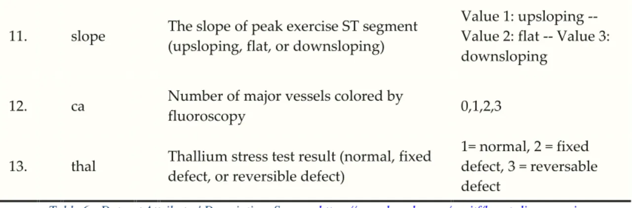
The attributes in the dataset and their description can be found in Table 6 in the appendix (chapter 10).

The machine learning Java application consists of two classes. The first class is

ModelGenerator and it takes the responsibility of generating the model using 4 methods; loadDataset to load the dataset from the ARFF file and saving it to an Instances object, buildClassifier method that builds the classifier for the training set using NaiveBayes

class (Naive Bayes Classifier), evaluateModel function that evaluates the accuracy of the generated model using the test dataset, and finally the saveModel function that saves the model in a .bin extension file for future uses.

In the Main class, ModelGenerator class is called by creating an object, loading the dataset file from its path to create instances from each line, and after that is randomizing and normalizing the dataset to improve the accuracy of the model.

Later, two objects of Instances class are created, one for the training dataset and the other is for the testing dataset, and an object of NaiveBayes class is created to build the classifier from the training dataset. Later, the classifier is evaluated by passing the model, training dataset, and testing dataset to the ModelGenerator object, and later the model is saved for future evaluation of new instances.

To get a better look into the classification performance of the ML application, the test dataset instances in the ARFF file below the @data tag were copied and pasted multiple

(20)

20

times to be 1508940 lines instead of 270. The same is done to the test dataset for the TP program, both have the same number of lines but different files sizes since ARFF uses different separators and different encoding, therefore, the ARFF file size is 109MB. In conclusion, the machine learning Java application as found in the literature study takes a dataset containing attributes and class values as an input, and the output of the application is the generated model which can be used to evaluate the model accuracy against a testing set or to classify new instances. The application source code can be found in the appendix (chapter10).

4.5 Traditional Programming Implementation

The first step in creating a traditional program is to collect information about the problem, the input, and the desired output in order to write an algorithm that handles the calculations and produce that output.

In the first attempt, Bayes' theorem was considered as a potential solution to the heart disease prediction problem since it handles the probabilities of an event based on prior knowledge of the condition, in our case, we use a person’s age to know the probability of him/her having a heart disease. Calculating the probability of a person having heart disease (sick) from the input (dataset) available [17] is calculated as the following:

P(sick|<age, sex, cp, trestbps, chol, fbs, restcg, thalach, exang, oldpeak, slope, ca, thal>) = (P(sick)*P(sick,age)*P(sick,sex) *P(sick,cp)*P(sick,trestbps)*P(sick,chol)*

P(sick,fbs)*P(sick,restcg)*P(sick,thalach)*P(sick,exang)*P(sick,oldpeak)*P(sick,slope) *P(sick,ca)*P(sick,thal)) / P(age, sex, cp, trestbps, chol, fbs, restcg, thalach, exang, oldpeak, slope, ca, thal)

where (age, sex, cp, etc.) are the variable input, and P(sick) is the probability of having heart disease and P(sick,age) is the probability of being at the given age and having a heart disease. Since Bayes’ theorem considers all probabilities are conditionally independent, the probability of being at the given age and being sick is independent of gender, cholesterol levels, fasting blood sugar, etc. Attributes description can be found in Table 6 in the appendix (chapter 10).

During an interview through a third-party conducted on 29 June 2019, Dr. Taisir Qahwaji, a senior interventional cardiologist at the Specialty Hospital in Amman, Jordan, stated

(21)

21

that it is not realistic or even possible to know the exact probability in the percentage for having a heart disease based solely on the age alone or the gender alone and so on for the rest of the input values as independent values from a medical perspective. Furthermore, heart disease diagnosis needs linked factors and examination results where one is strongly dependent on the other. Naive Bayes can still yield good results if dependencies between attributes cancel each other out or if they are distributed evenly [7]. Exact percentages can be calculated form the dataset; however, this approach would result in Naive Bayes classifier that is hardcoded, it would still be machine learning approach, but with training part done by developer.

After dismissing Bayes’ theorem, the traditional program created to classify the data consists of two classes. The first class is the HeartData class where it has a list of the required inputs for the classification, a constructor, and classify method.

In classify method, a set of if-else statements are created to handle the input and decide whether the line of data from the CSV file is a patient with heart disease or not based on the cardiologist notes about the strong indicators of heart disease presence while dismissing the values of uncertain indicators like slope, maximum heart rate since it is related to the age and physical activity routine and smoking, and fasting blood sugar since high values indicate a high probability of getting a heart disease in the future but not the presence of heart disease in the present due to internal organ damage.

A list of dangerous values which indicates that a patient is sick was given by Dr. Taisir, where he explained the factors that are strong indicators of having a heart disease based on the attributes available in the dataset, where he also noted that is not enough to be certainly sure. The full interview conversation is written in the appendix (chapter 10). The second class in the application is the TProgram class where the main method is written, which is the entry point of any Java program. In the main method, OpenCSV library is imported to handle the CSV file parsing, which is an easy-to-use library that supports all basic methods to handle CSV files. CSVReader object from the OpenCSV library is created to parse the dataset CSV file where an object is created from the values parsed from one line and passed to the HeartData constructor to create an object of

HeartData.

A while loop compares the result returned by the classify method (the predicted class value) with the 14th attribute in the dataset (the correct class value). If both are equal, then

(22)

22

we check if it’s a true positive or true negative, while if the predicted and the correct values aren’t equal, we add them to the respected category, either false positives if the person is actually sick and the predicted value is healthy, or false negative if the person is actually healthy and predicted to be sick. Finally, displayApplicationStats method is called to calculate and display the total accuracy, precision, and recall results, in addition to calculating the execution time of the program using Time Java library.

The execution time of the traditional program is almost instantaneous, and to get a better look into the classification performance, the dataset instances inside the CSV file were copied and pasted many times to be 1508940 instead of 303 where the CSV file size became 53.3 MB. The application source code can be found in the appendix (chapter 10).

(23)

23

5. Results

5.1 Development Time

The code implementation of the traditional programming approach was done in two days, on the first day, the response from the cardiologist was organized and divided to produce a set of consecutive if-else statements to handle the input data, and the second day tasks were to experiment and tweak the code to make it as fast and resource-friendly as possible.

However, a long period of time (approximately 1 month) was assigned to study the heart disease problem, the dataset and its attributes to be able to communicate with the cardiologist with a basic understanding of the input values, and finally the time it takes to find a patient cardiologist willing to read the case, exchange messages and answer further questions, and to simply list all readings that indicate if a patient is having a heart disease or not with approximate probabilities of the disease occurrences based on the available attributes in the dataset. Note that the dataset used is ready-to-use dataset where the developers did minimal modifications to it and didn’t have to deal with feature selection, noise in data, or empty values.

The development time of the machine learning approach was longer than the traditional program one. Since the developers had no previous experience with ML before, it took time to read about the subject and understand the ML applications and supervised learning algorithms.

The total development duration of the ML was approximately 10 weeks, taking in hand that the dataset is ready to use after some minor modifications. It would take a longer time if the developers had to collect data themselves because of many factors like dealing with noise in data and missing values, and the features selection process. Feature selection is the process of removing redundant and irrelevant attributes which will improve learning accuracy and reduce training time.

In addition, the developers didn’t create their own algorithm to deal with the problem, instead, they reviewed two popular ML algorithms (SVM and Naive Bayes) applied to the heart disease dataset and compared their performances from the literature review and testing with WEKA GUI Workbench to choose the best one for the chosen dataset.

(24)

24

5.2 Code and Time Complexity

The number of lines in an application’s code is one of the oldest and most common methods to measure the code complexity. A large number of lines (code size) usually indicates that the application has many operations or calculations, and also indicates that the application code is hard to maintain. However, the number of lines isn’t always enough to get a full preview of the code complexity, therefore, other important factors should be considered like coupling, lack of cohesion and complexity.

Coupling between the application classes is a factor that affects the code complexity and it happens when a class has an attribute referring to another class, has a method that reference the other class, or a class has a local instance of another class. Tightly coupled classes indicated higher complexity, where any single change to one class can affect and change other classes, and it makes the class harder to reuse since all the classes coupled with it must be included.

Lack of cohesion is another factor that indicates the code complexity, where it is the measurement of the relation between methods in the same class and if there any dependence between them. Low lack of cohesion is desirable since it makes the code easy to comprehend, more robust and able to be reused in other parts of the software.

The complexity of the interaction between the application’s entities also affects the overall code complexity since it makes the code more prone to defects caused by changes in the software that changed the internal interaction between the software’s entities. Running CodeMR tool in an Integrated Development Environment (IDE) produces a detailed table of metrics for the application and the results of the traditional programming and the machine learning applications is shown in Table 1 and Table 2.

CLASS COMPLEXITY COUPLING LACK OF COHESION SIZE

HeartData low-medium low low low

TProgram low low low low

(25)

25

CLASS COMPLEXITY COUPLING LACK OF COHESION SIZE

ModelGenerator low low-medium low low

Main low low-medium low low

Table 2 - ML Code Complexity Metrics Produced by CodeMR

The total number of lines in the two classes created in the TP application is 68 lines, and 12 external classes are used. While the total number of lines in the two classes created in the ML application is 60 lines, and 26 external classes are used.

For the time complexity, all instructions in the traditional program apart from loops are of time complexity of O(1), where there is only one for loop in the code that goes through the dataset CSV file lines, thus, the time complexity of the application in Big-O notation is O(n), where n is the number of lines in the CSV file.

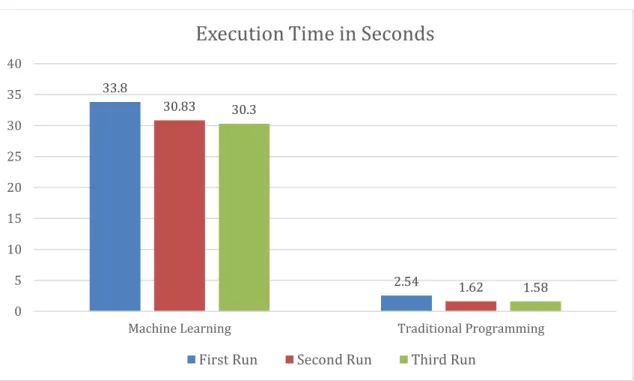
The execution time in the first run of the application after starting the IDE is 2.54 seconds, for the second run it is 1.62 second and the third run is 1.58 second to classify the multiplicated version of the dataset with a size of 53.3MB. The recorded execution times for the first run or the later runs aren't constant values and can slightly vary on each run since it’s not possible to get the same exact value in every run (as found in section 2.4), especially on a different machine than the one that is running the IDE. In all trials, the first run execution time was slightly longer than the second and third runs.

For the machine learning application, the NaiveBayes class in WEKA library contains multiple for loops, however, one nested loop was found. There is one while loop used in building the classifier that has a for loop inside it. Calculating the time complexity of it is O(nK), where n is the number of training instances and K is a constant number of attributes.

In real-world cases, the number of attributes isn’t as big as the number of instances even in multidimensional classification problems and it is fixed compared to the variable

(26)

26

number of test instances, therefore, the time complexity is related to the linear time complexity O(n) for training and for testing.

The execution time for the ML application on the first run where the model wasn’t created (training and testing) is 33.8 seconds, and when the model was available to use instead of training a new one in the second run was 30.83 seconds, and the third run was 30.30 seconds for classifying the duplicated test dataset of size 109MB. While for the original test dataset (no duplication) scored an execution time of 0.246 of a second on the first run (with creating the model), 0.238 second in the second run, 0.235 of a second on the third run where the model is present. Side by side comparison is shown in Figure 3.

Figure 3 – Execution time difference between ML and TP

5.3 Classification Accuracy

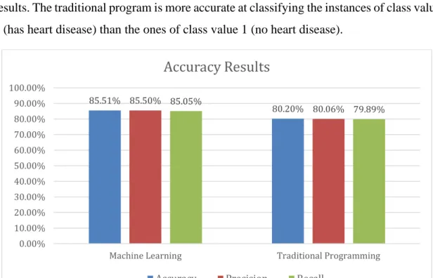
Naive Bayes algorithm in the machine learning application landed an accuracy of 85.51% (correctly classified instances), taking in mind that the training set contains 303 instances while the number of unique instances in the test dataset is 270.

33.8 2.54 30.83 1.62 30.3 1.58 0 5 10 15 20 25 30 35 40

Machine Learning Traditional Programming

Execution Time in Seconds

(27)

27

The accuracy of the classification is the number of correctly classified instances (true positives + true negatives) to the total number of instances (true positives + true negatives + false positives + false negatives):

𝐴𝑐𝑐𝑢𝑟𝑎𝑐𝑦 = 𝑇𝑃 + 𝑇𝑁

𝑇𝑃 + 𝑇𝑁 + 𝐹𝑃 + 𝐹𝑁

However, the classification accuracy alone isn’t enough to determine the classification performance. To investigate deeper in the classification accuracy, precision and recall should be calculated.

Precision is the ratio of the correctly classified instances (true positives) in single class value to all instances that were classified to the same class value (true positives + false negatives) [25], which answers the question of how many instances that were classified as sick are actually sick.

𝑃𝑟𝑒𝑐𝑖𝑠𝑖𝑜𝑛 = 𝑇𝑃 𝑇𝑃 + 𝐹𝑃

Recall (also known as sensitivity) is the ratio of the correctly classified as a single class value to the number of all instances in that class value [25], which means how many correctly classified as sick from the total number of sick instances.

𝑅𝑒𝑐𝑎𝑙𝑙 = 𝑇𝑃 𝑇𝑃 + 𝐹𝑁 The precision and recall results are shown in Table 3.

Precision Recall

Class value 1 – no heart disease 85.4% 89.2%

Class value 2 – has heart disease 85.6% 80.9%

Table 3 - ML precision and recall ratios for class values 1 and 2

The precision ratios for both class values are close to the accuracy while the model sensitivity to class value 1 is considerably higher, which means the application is more accurate at classifying no heart disease instance than with heart disease instances.

(28)

28

The traditional programming (TP) application scored an accuracy of 80.2%. A possible justification for scoring less accuracy than the ML application is that the attributes in the dataset aren’t enough to determine if the person is sick or not as the cardiologist asked for more information like if the person is a smoker, obese, genetic conditions, glycated hemoglobin test, diabetes duration, etc. In addition, to cover every possible case of sickness needs a group of dedicated cardiologists to list it, which isn’t possible for the time or budget given to this thesis.

The precision and recall of the traditional program classification are shown in Table 4. Precision Recall

Class value 1 – no heart disease 78.68% 77.54%

Class value 2 – has heart disease 81.44% 82.42%

Table 4 - TP precision and recall ratios for class values 1 and 2

While the precision is close in value to the accuracy, we notice the difference in the recall results. The traditional program is more accurate at classifying the instances of class value 2 (has heart disease) than the ones of class value 1 (no heart disease).

Figure 4 - Accuracy difference between ML and TP 85.51% 80.20% 85.50% 80.06% 85.05% 79.89% 0.00% 10.00% 20.00% 30.00% 40.00% 50.00% 60.00% 70.00% 80.00% 90.00% 100.00%

Machine Learning Traditional Programming

Accuracy Results

(29)

29

5.4 Resource Consumption

Using the original test datasets did not lead to records that the difference can be detected, therefore, for all the following test the duplicated test datasets were used to capture the difference clearly.

The resources consumption of both applications was recorded using JProfiler v11.0.1 plug-in in the following environment:

IDE: IntelliJ IDEA 2019.1.4 (Ultimate Edition) JRE: 1.8.0_212-release-1586-b4 amd64

JVM: OpenJDK 64-Bit Server VM by JetBrains s.r.o Windows 10 Home Edition, version 1903.

The Hardware specification of the machine:

CPU: Intel Core i7-4700HQ 2.4GHz up to 3.40GHz, 4 cores 8 threads, 6MB cache. Memory: 8GB DDR3L dual-channel, DRAM frequency 1600MHz.

Storage: Samsung SSD 860 EVO, 550 MB/sec reading speed, 520 MB/sec writing speed.

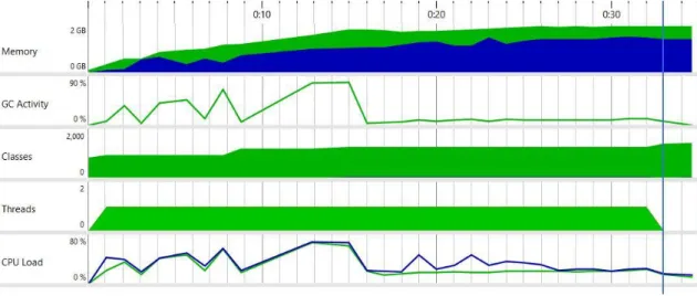
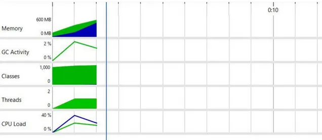
The difference between the machine learning (ML) application and the traditional programming one for resource consumption is huge, as shown in Figure 5 and Figure 6.

(30)

30

Figure 6 - TP application resource consumption captured using JProfiler

WEKA library wasn’t designed to handle large files and the maximum dataset file size found to be working is 109MB, while another experiment with a 150MB file didn’t succeed due to OutOfMemoryError even though the heap size is set to 2048MB.

However, the traditional program can handle large data since it is using OpenCSV library that can stream the data in the CSV file to the memory instead of loading all of it at the run time. Note that both applications are single-threaded.

The maximum values reached during the test are in Table 5.

CPU Load Memory Usage GC Activity Classes Loaded

TP 19.15% 442 MB 1.9% 937

ML 68.81% 1515 MB 83.14% 1477

(31)

31

6. Analysis

The development time is relative, and it is affected by the developer’s experience in the field and the complexity of problem. In the assumption that a developer is well experienced in both ML and TP, the traditional programming approach would take longer since it needs a deeper understanding of the scope of the problem.

The process of collecting the information related to solve the problem isn’t always an easy task and, in some cases, it cannot be acquired from online searches. A consultation with an expert in the field of the problem is essential, where both developers and specialists can discuss the problem to form a common ground of understanding which will give the developers the essence of information needed to create an algorithm to produce the solution. While in the machine learning approach, the developer needs to try multiple algorithms to find the most accurate one dealing with the given dataset.

The metrics result produced by CodeMR showed that the complexity of TProgram class in the TP application is higher in complexity than the HeartData class in the same application, and more complex than both classes in the ML application. Whereas the coupling in the ML application’s two classes is higher than the TP application’s classes. The rest of the results are in the same category (low) for both applications.

Both ML and TP solutions are in the linear time complexity. Since both are running on the same hardware, it is obvious that O(Kn) is larger than O(n) which is one reason that the execution time of the ML solution was longer. The other reason for the slower execution is the garbage collection activity.

As shown in Figure 7, the garbage collection activity (GC Activity) had multiple spikes during the execution. These multiple spikes indicate that the GC activity started multiple times, which also means that the application has gone through multiple pauses in execution (stop-the-world) in order to secure the integrity of the object trees [26]. The GC is affected by the number of alive objects rather than the dead ones, so the more alive objects, the longer GC activity lasts.

The Naive Bayes conditional independence assumption that is seldom valid in real-world classification problems, and that is the reason why Bayes’ theorem wasn’t possible to implement in the TP application. It is impossible to get ratios for conditionally independent attributes related to heart disease detection from a medical perspective as the

(32)

32

cardiologist stated, and it is vital to remember that Naive Bayes is a probabilistic classifier. The probabilities ratios calculated in the ML application are from the training dataset alone where it calculated the posterior probability based on the values in the training dataset, not from global statistics or medical information. The dataset is collected from a small number of patients from small number of hospitals; therefore, it cannot give a global insight over heart diseases in all parts of the world since it can be affected by the race, genetics, environment, and lifestyle.

The ML Naive Bayes accuracy of 85.5% is considered good since the training dataset is relatively small and the strong connection between attributes in a heart disease classification task. Naive Bayes is optimal and gave good results since strong dependencies cancel each other without any influence on the classification [27].

Naive Bayes gave good results, but the accuracy cannot be improved unless the training dataset is changed to another with more instances. Swapping the datasets where the training dataset is the 270 instances and the 303 one is for the testing, Naive Bayes accuracy dropped to 70%. Therefore, a larger training dataset can improve the accuracy of the Naive Bayes classifier. Additionally, the accuracy results findings in this thesis (chapter 5) contradict with researches [12] and [13] accuracy results, even when using cross-validation with10 folds option or percentage split option.

The traditional programming application can only get more accuracy if it had access to more attributes and longer consultation sessions with cardiologists which also mean modification to the program and its classification method.

The ML application was not a resource-friendly application because of the high CPU and memory usage. Alongside the high CPU load, the execution time is also long which means more power consumption than the traditional program application.

(33)

33

7. Discussion

The findings of this study proved that the traditional programming application scored better performance results except in the classification accuracy. The one case where the TP application is the preferable approach for implementation is if the company needs a classification program with a single purpose, to classify a single type of data with a constant number of attributes.

A consultation with an expert in the field is needed to determine if high accuracy is achievable. The TP application is more sustainable since it uses less amount of power and classifies data in significantly less time than ML. The accuracy of the TP may score better if additional attributes are added, but the dataset with full attributes suffers from corruption and lots of missing values.

In other cases where a company needs multiple types of classification where the data attributes can be changed over time, it is better to implement a machine learning, because of its ability to adapt to new attributes in less effort than the TP approach. Machine learning classification is significantly slower than the TP application, and it can be even slower, especially in training time, if an algorithm of higher time complexity is implemented like SVM.

The popularity of WEKA is related to training and testing smaller datasets in size, whereas shown in the results, WEKA developers didn’t create the libraries to handle large datasets (larger than 150MB dataset files) nor to have better memory management regarding the garbage collection activities that need additional tuning.

Naive Bayes training time is 0.12 second using the 303 instances dataset.

7.1 Ethical Issues and Sustainability

This study used healthcare data collected from patients at the time of admission to a hospital where they appeared to have heart disease and later, they were thoroughly inspected and diagnosed with either having heart disease or not. The dataset used in this thesis is derived from a larger one with 76 attributes and was collected from multiple institutes in 1988. The original dataset held much information about the patient's health records in addition to the patient real full name and social security number. It was published as a public dataset for developers and researchers to use, while it contained

(34)

34

private information about the patients. This is an example of a confidentiality violation, as stated in the dataset description, the patients' names and social security numbers were removed recently.

The ethical issues of mass data collection were brought to light by Edward Snowden in 2013 where he leaked classified information about the National Security Agency's mass surveillance. A deeper analysis of the Big Data ethical challenges was published by Crawford, Miltner, and Gray [28] where they showed the impact of Big Data on the economy and politics where they listed an example of the low cost of mass surveillance published by Bankston and Soltani (2014).

Big Data analysis technologies create a line in society between people that their data is being collected and the people who are capable of analyzing that data, which gives the latter more power and control over the rest.

Crawford, Miltner, and Gray continue with their critique that people are forced to accept the terms and agreements of large corporations or else they would have to withdraw from technology. Data isn’t always safe, it can be sold to other companies [29] or face the risk of leakage due to errors, hacks, or whistleblowing [30][31].

The data required to train a machine learning model to detect heart disease doesn’t require the patients’ personal information and patients should agree on their data being used for scientific research that can help others. The larger the dataset the better accuracy it yields, but it is still prone to classification errors and false negative values where it shouldn’t create a bias in the patient diagnosis.

Machine learning can provide help with early heart disease detection; however, a lot of improvements should be done before a disease detection system can be deployed for general use. A large training dataset is the most important part that should be acquired first, then multiple algorithms should be tested to get the highest possible accuracy. Both TP and ML application are not a replacement for professional cardiologists and should not be the only measure taken in diagnosing heart disease.

The traditional programming approach doesn’t require training or testing datasets, and only requires the knowledge of experts in the field. In addition, it is a better approach regarding sustainability since the lower resource consumption compared to the machine learning application created in this thesis.

(35)

35

8. Conclusion

The case presented in this thesis was able to be solved in both ML and TP with different performance and accuracy measures, it is one of a few cases where ML and TP can be applied. And it is important to mention that each approach has its field of problems that cannot be solved by the other one, like control and critical software that is dominated by the traditional programming approach since it needs fast reaction time and strict results with zero-error values. While the machine learning approach is dominant in the field of image and voice recognition and data mining. In plain English, the model created in the machine learning application serves the same purpose as the classify method in the traditional programming application and the main difference is that the model is created by learning from the dataset, while the classify method classification conditions are hard-coded where the conditions are implemented by the developers with the help of a cardiologist. As shown in Figure 1, we agree that the model is the output of the ML application that can in a later step be used to classify data, while the TP application doesn’t generate such a model, instead, the conditions for classification is present within the code.

The traditional programming approach is proved to have better overall performance except for the accuracy in this thesis. The results proved that TP executes faster, less complex, and more resource-friendly, while the machine learning approach is proved to have better accuracy results in heart disease detection and doesn’t require knowledge in the field of the problem in order to be able to classify the data.

The TP accuracy can only get more accurate in the case of adding more attributes and changing the classification method to handle the new relation between the new attributes with the old ones. And machine learning accuracy can only get better when using a dataset with a larger number of attributes, and possibly better if another algorithm is implemented which needs further trials to choose the best suitable algorithm.

Bayes' theorem cannot be applied to the heart disease problem in traditional programming since the attributes are strongly dependent and the probability of a single independent probability isn’t realistic in the field of cardiology and no known ratios are available. While in machine learning, the Naive Bayes algorithm that is based on Bayes' theorem proved to yield good accuracy even when attributes are strongly dependent.

(36)

36

8.1 Future Work

Future work on this study could resolve some of the following areas of improvements: • Additional longer interviews with a cardiologist that can possibly improve the

accuracy of the traditional program classification.

• Modification to WEKA library to be able to handle larger datasets and further tunings into its memory management and garbage collection mechanisms. • Modifications to WEKA can also be used to reduce resource consumption to make

the machine learning application more energy-efficient.

• Investigate other machine learning frameworks that handle larger datasets, like Apache Spark and their performance regarding energy consumption.

(37)

37

9. Bibliography

1. A Gentle Introduction to Deep Learning — [Part 1 ~ Introduction] [Internet]. Medium. 2019 [cited 10 August 2019]. Available from:

https://towardsdatascience.com/a-gentle-introduction-to-deep-learning-part-1-introduction-43eb199b0b9

2. Gulli A. Deep learning with Keras. 2017.

3. Aggarwal, Charu C. Data Classification: Algorithms and Applications. CRC Press. 2015.

4. Wolpert D, Macready W. No free lunch theorems for optimization. IEEE Transactions on Evolutionary Computation. 1997;1(1):67-82.

5. UCI Machine Learning Repository [Internet]. Archive.ics.uci.edu. 2019 [cited 10 August 2019]. Available from: https://archive.ics.uci.edu/ml/index.php

6. Georges A, Buytaert D, Eeckhout L. Statistically rigorous java performance evaluation. ACM SIGPLAN Notices. 2007;42(10):57.

7. Zhang H. The optimality of naive Bayes. In Proceedings of 17th International Florida Artificial Intelligence Research Society Conference. 2004. 562–567. 8. Parsian M. Data Algorithms. Beijing: O'Reilly Media, Inc.; 2015.

9. Rish I. An empirical study of the naive bayes classifier. In: On the move to meaningful internet systems 2003: CoopIS, DOA, and ODBASE. OTM 2003. Lecture notes in computer science. Berlin: Springer; 2003. pp. 986–96.

10. Domingos P., Pazzani M. On the optimality of the simple Bayesian classifier under zero-one loss. 1997.

11. Nashif S, Raihan M, Islam M, Imam M. Heart Disease Detection by Using Machine Learning Algorithms and a Real-Time Cardiovascular Health Monitoring System. World Journal of Engineering and Technology. 2018;06(04):854-873.

12. Anbarasi M., Anupriya E., Iyengar N.C.S.N., Enhanced Prediction of Heart Disease with Feature Subset Selection using Genetic Algorithm, International Journal of Engineering Science and Technology Vol. 2(10), 2010, pp. 5370-5376.

13. Masethe HD, Masethe MA. Prediction of heart disease using classification algorithms. In: Proceedings of the world congress on engineering and computer science. San Francisco: WCECS; 2014. p. 22–4.

(38)

38

14. Miao H. K, Miao H. J, Miao J. G. Diagnosing Coronary Heart Disease using Ensemble Machine Learning. International Journal of Advanced Computer Science and Applications. 2016;7(10).

15. Green W. Machine Learning with a Heart: Predicting Heart Disease [Internet]. Medium. 2019 [cited 28 March 2019]. Available from:

https://medium.com/@dskswu/machine-learning-with-a-heart-predicting-heart-disease-b2e9f24fee84

16. UCI Machine Learning Repository: Statlog (Heart) Data Set [Internet]. Archive.ics.uci.edu. 2019 [cited 11 August 2019]. Available from:

https://archive.ics.uci.edu/ml/datasets/Statlog+%28Heart%29

17. 12. Heart Disease UCI [Internet]. Kaggle.com. 2019 [cited 11 August 2019]. Available from: https://www.kaggle.com/ronitf/heart-disease-uci/version/1 18. Abdiansah A, Wardoyo R. Time Complexity Analysis of Support Vector

Machines (SVM) in LibSVM. International Journal of Computer Applications. 2015;128(3):28-34.

19. Tsang W, Kwok J. T., Cheung P.M. Core vector machines: Fast SVM training on very large data sets. Journal of Machine Learning Research6, Apr (2005), 363– 392.

20. Piatetsky G. Python eats away at R: Top Software for Analytics, Data Science, Machine Learning in 2018: Trends and Analysis [Internet]. Kdnuggets.com. 2019 [cited 5 May 2019]. Available from: https://www.kdnuggets.com/2018/05/poll-tools-analytics-data-science-machine-learning-results.html/2

21. Witten I, Frank E, Hall M, Pal C. Data mining. 4th ed. 2016.

22. Attribute-Relation File Format (ARFF) [Internet]. Cs.waikato.ac.nz. 2019 [cited 10 May 2019]. Available from: https://www.cs.waikato.ac.nz/ml/weka/arff.html

23. 10 Popular Java Machine Learning Tools & Libraries [Internet]. Datasciencecentral.com. 2019 [cited 29 July 2019]. Available from:

https://www.datasciencecentral.com/profiles/blogs/10-popular-java-machine-learning-tools-libraries

24. [Internet]. Ej-technologies.com. 2019 [cited 1 August 2019]. Available from: