Evaluation of data from a pilot scale pebble mill
Johanna Alatalo1, Bertil Pålsson1 and Kent Tano2
1 Div. of Minerals and Metallurgical Engineering, Luleå University of Technology, Sweden 2 Research and Development, LKAB, Sweden
Abstract
Autogenous grinding is a process of reducing the particle size distribution of an extracted ore by using the ore itself as grinding media. It is a process that is very difficult to control and there is also a lack of knowledge of the events occurring inside the mill. To find out more how the mill behaves under different process conditions a full factorial test were performed with a iron ore in a pilot scale mill at the LKAB R&D facility in Malmberget. As a
complement a strain gauge detector was embedded in one of the mills rubber lifters, the Metso Minerals CCM system, and it is used to get more information about the charge dynamics. The data from the experiments has been analysed with the aid of a statistical program. For production purposes an increase of the amount less than 45 µm can be regarded as a probable increase of production rate. The analysis shows that there will be an increase of fines at 65 % of critical speed especially when the mill has a 45 % filling degree. This setting will also increase the power consumption but improves the grindability of the ore even more. A higher degree of filling also give a smaller toe angle and a higher shoulder angle as
expected.
Introduction
Autogenous grinding is a process letting the ore itself reduce the particle size distribution of an extracted ore. This is a very complex and expensive process. It is complex due to the many factors that affect the process. Firstly, the result is very strongly dependent on the size
distribution of the ore fed to the mill (Fahlström, 1962). Also, the chemical properties of the ore influence the process and the feed rate regulates the mill properties. Finally, most settings need to be finely tuned for an optimal grinding process.
The mills have high power consumption and most energy will not be used to ground the material, less than 10% is used for grinding (Tano, 2005). There are large economical benefits to be made with improved and optimised grinding settings. However, since the ore to a
concentrator varies; the grindability of an ore is not constant over time. The chemical content and the physical properties may vary and results in varying optimal operating conditions for the mill settings.
This means that autogenous grinding is a process that is difficult to control and there is also a lack of knowledge of what happens inside a mill. Since the environment inside the mill is too harsh for direct measurement, and to get a better understanding of a mill's performance alternative measurement systems are necessary. This can be by done for example by measuring vibrations with sensors placed on a mill shell (Campbell, 2001), by the use of inductive sensors placed inside the mill (Kiangi, 2008) or by using an acoustic method (Pax, 2001) to get information of events inside a mill. Different sensors have been made,
Magoutteaux has developed a mill sensor SensoMag (Clermont 2008) and the CCM (Continuous Charge Measurements system) by Metso minerals has been shown to have features as good reproducibility, reliability and a fast response time for varied process
conditions (Tano 2005). The CCM system is used here in an attempt to learn more about the charge dynamics in the experiments discussed in this article.
Most controlled experiments are performed with lab-scale mills. At the University of Cape Town, a lab-scale mill was investigated by X-ray filming (Powell, 2003) and gave very detailed information about the movements in that mill. A slightly larger mill had a diameter of 90 cm and a length of 15 cm has also been used (Rajamani, 2000). The use of the smaller mills is of course a limitation, but larger mills are more difficult to control and more noise is introduced in the data. Despite this, the pilot scale mill that is used in the experiments mentioned in this article is approximately 1.4x1.6 m.
Scope of works
It is of interest to increase the production from the mills, and one way of doing this is to optimise the mill settings. However, it is important to first enhance the understanding of how the mill behaves under different process conditions. To investigate the behaviour a full factorial test was performed. The different factors were weight % solids, mill filling level and the rotational speed of the mill. They were varied between 60 % to 65 % weight % solids, between 35% and 45% filling by volume and 73 % and 78 % of critical speed. The charge medium consisted of 50 % magnetite pebbles and 50 % gangue pebbles by volume.
The experimental setup
LKAB has at their R&D facility in Malmberget, Sweden, a pilot mill which is used to obtain the necessary experimental data. The grate-discharge mill is approximately 1.4 m in diameter and 1.57 m in length and has 12 rubber lifters installed. The lifters are 10x10 cm and have a face angle of 45 degrees. There is a rubber lining. The mill is controlled from a process
control room, and from where it is also possible to control the feed to the mill, the pebble- and the water addition. The speed of the mill requires a change of the size of the pulleys. This mill has been used previously when different settings with a steel ball charge were investigated (Tano, 2005).
In one rubber lifter, a strain gauge detector is embedded, see Figure 1. This detector is a part of the Continuous Charge Measuring (CCM) system from Metso Minerals. As the lifter bends backwards, the strain gauge mounted on the leaf spring converts the deflection to an electric signal. The signal is then amplified, filtered and transmitted to a computer (Dupont 2001). When the CCM is operating, the speed, charge level, toe-, shoulder- and charge angles and a deflection signal are continuously updated in the CCM monitoring program. The sensor is very sensitive to changes in operating conditions and has also shown good reliability and fast response time (Tano, 2005). All this information is of great value when performing
Figure 1. A cross section of the rubber lifter with at strain gauge detector embedded and a view inside the mill with the lifters.
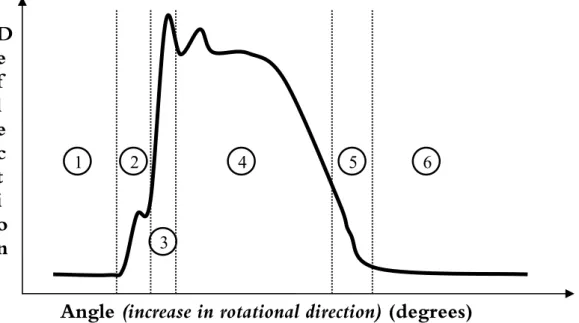
The signal from the CCM system contains much information about the performance of the mill. A typical deflection profile can be seen in Figure 2. It is also possible to perform calculations on the signal to get even more data, such as charge volume.
Figure 2. A simplified view of a typical deflection signal of one revolution from the CCM system. A typical signal of one revolution can be described with a few positions. First the lifter is in the air and unaffected, position 1.Then it will reach the toe area, position 2. The toe area commonly shows some turbulence and here it is also possible to detect slurry pooling. When the lifter hits the charge, the deflection increases rapidly and normally reaches the maximal deflection at the bottom of the mill, position 3. As the lifter continues to move through the charge, the shockwaves from other lifter impacts can be detected, position 4. The deflection decreases as the mill leaves the charge, which is referred to as the shoulder area, position 5. Finally the lifter retracts from the charge and returns to its normal position, i.e. position 6.
D
e
f
l
e
c
t
i
o
n
Angle (increase in rotational direction) (degrees)
1 2
3
Experimental conditions
The feed to the mill was a magnetite pellet feed with at d50 of approximately 35µm and a
density of 4.8 ton/m3. The feed rate was kept constant at 0.85 ton/h to get a size distribution similar to the full scale pebble mills at LKAB:s facilities at Kiruna, Sweden.
The charge consisted of a mixture of magnetite and gangue pebbles, 50% by volume. The pebble feed rate was set to approximately 0.14 ton/h to maintain a constant volume % filling in the mill. The pebbles were between 10-35 mm in size. The setup is shown in Figure 3.
Figure 3. The experimental setup.
Result
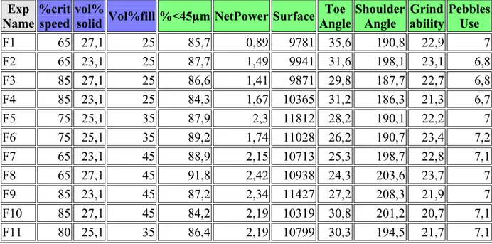
The full factorial test, with centre points is analysed with the aid of a statistical program, MODDE. The factors are the degree of filling (volume % filling), the % of critical speed and the volume-% solids. Data from the experiments are given in Table 1. The responses are: %<45 µm in Product, measured NetPower (kW), specific surface area (cm²/cm³) for Product, Toe and Shoulder angles in degrees, Grindability (kg <45 µm/kWh net), Pebbles Use
(kg/kWh net). Note, that experiment F11 should have been done at 75 % of critical speed, but landed on 80 % due to an error in changing pulleys. When analysing the data, the interaction effects from volume-% solids has been excluded, due to the low significance of volume-% solids as a main effect.
Table 1. Data from experiments. Exp
Name %crit speed vol% solid Vol%fill %<45µm NetPower Surface AngleToe Shoulder Angle ability Grind PebblesUse
F1 65 27,1 25 85,7 0,89 9781 35,6 190,8 22,9 7 F2 65 23,1 25 87,7 1,49 9941 31,6 198,1 23,1 6,8 F3 85 27,1 25 86,6 1,41 9871 29,8 187,7 22,7 6,8 F4 85 23,1 25 84,3 1,67 10365 31,2 186,3 21,3 6,7 F5 75 25,1 35 87,9 2,3 11812 28,2 190,1 22,2 7 F6 75 25,1 35 89,2 1,74 11028 26,2 190,7 23,4 7,2 F7 65 23,1 45 88,9 2,15 10713 25,3 198,7 22,8 7,1 F8 65 27,1 45 91,8 2,42 10938 24,3 203,6 23,7 7 F9 85 23,1 45 87,2 2,34 11427 27,2 208,3 21,9 7 F10 85 27,1 45 84,2 2,19 10319 30,8 201,2 20,7 7,1 F11 80 25,1 35 86,4 2,19 10799 30,3 194,5 21,7 7,1 Magnetite pellet feed Water Pebble feed Chips Product Pebble mill
The summary of fit plot and the normal probability plots are shown in appendix 1. The coefficient plot, see appendix 2, show that the responses in most cases depend on the critical speed or on the degree of filling of the mill. The critical speed has a significant effect on the amount less than 45 µm and on the grindability. The degree of filling has a significant effect on the net power consumption, the specific surface area, the toe and shoulder angles and the pebbles consumption.
Critical speed
The effect of changing the rotational speed of the mill influences the amount of fine material produced and the grindability of the ore. It can be seen in Figure 4 that for a lower percentage of critical speed, the amount of < 45 µm and the grindability increases compared to those at a higher percentage of critical speed. The amount of < 45 µm increases with almost 3 % and the grindability increases with almost 1.5 kg < 45 µm/ kWh net when the speed is at 65 % of critical speed instead of 85 % of the critical speed. This indicates that a better production results will be the case when a low percentage of critical speed is used, i.e. the lower rotational speed gives better grinding condition.
85 86 87 88 89 90 64 65 66 67 68 69 70 71 72 73 74 75 76 77 78 79 80 81 82 83 84 85 86 % <45µ m %critspeed
Main Effect for %critspeed, resp. %<45µm
N=11 R2=0,639 R2 Adj.=0,399 DF=6 Q2=-0,756 RSD=1,724 Conf. lev.=0,90 21 22 23 24 64 65 66 67 68 69 70 71 72 73 74 75 76 77 78 79 80 81 82 83 84 85 86 G rin da bilit y %critspeed
Main Effect for %critspeed, resp. Grindability
N=11 R2=0,631 R2 Adj.=0,385
DF=6 Q2=-0,517 RSD=0,7255 Conf. lev.=0,90
MODDE 8 - 2011-01-26 12:14:02
Figure 4. The main effect plots for critical speed on amount < 45 µm and for grindability.
Volume % solids
For the volume % solids, see appendix 3, it is difficult to interpret the results since there are no obvious significant effects. This is most likely due to the too small difference between the high and low values for this factor; the variation in the volume-% solids was not large
enough. The original plan called for a larger variation, but due to process restraints the variation became too small. However, there is an indication that a higher volume % solids
will increase the grindability and also that the charge will climb higher in the mill. The result from Tano's experiments showed that the charge would have a lower toe angle and a higher shoulder angle at higher volume % solids (Tano, 2005).
Degree of filling
The main effect of lower or higher degree of filling in the mill can be seen in Figure 5. When the degree of filling of the mill is high, the net power consumption will increase. This is the expected result, since more material has to be rotated by the mill, i.e. more power is
necessary. With a high degree of filling the specific surface area and pebbles consumption increase.
The extra material in the mill also causes a change in toe and shoulder angles, which can be seen in the statistical data. The toe angle will be lower and the shoulder angle will be higher with a higher degree of filling.
1.5 2.0 2.5 24 26 28 30 32 34 36 38 40 42 44 46 N etP ow er Vol%fill
Main Effect for Vol%fill, resp. NetPower
N=11 R2=0,793 R2 Adj.=0,656 DF=6 Q2=0,270 RSD=0,2851 Conf. lev.=0,90 10000 10500 11000 11500 24 26 28 30 32 34 36 38 40 42 44 46 Su rf ac e Vol%fill
Main Effect for Vol%fill, resp. Surface
N=11 R2=0,435 R2 Adj.=0,059 DF=6 Q2=-0,603 RSD=633,2 Conf. lev.=0,90 6.8 6.9 7.0 7.1 7.2 24 26 28 30 32 34 36 38 40 42 44 46 P ebbl es U se Vol%fill
Main Effect for Vol%fill, resp. PebblesUse
N=11 R2=0,553 R2 Adj.=0,256 DF=6 Q2=-0,380 RSD=0,1326 Conf. lev.=0,90 26 28 30 32 24 26 28 30 32 34 36 38 40 42 44 46 T oeA ngl e Vol%fill
Main Effect for Vol%fill, resp. ToeAngle
N=11 R2=0,778 R2 Adj.=0,629 DF=6 Q2=0,139 RSD=2,001 Conf. lev.=0,90 185 190 195 200 205 24 26 28 30 32 34 36 38 40 42 44 46 S ho ul der A ngl e Vol%fill
Main Effect for Vol%fill, resp. ShoulderAngle
N=11 R2=0,753 R2 Adj.=0,588
DF=6 Q2=0,024 RSD=4,535 Conf. lev.=0,90
MODDE 8 - 2011-01-26 12:14:56
Figure 5. The main effect plots for volume % filling on the net power consumption, the specific surface area, the pebbles consumption and the toe and shoulder angle.
Interactions
The interaction plot show that a high critical speed will decrease the effect the filling has on the amount < 45 µm, see in the left graph in Figure 6. At a high speed there is almost no difference between in the amount < 45 µm when the mill filling is low or high. At a low speed, a high filling will give more material below 45 µm than a low filling degree. Here, one may speculate that a slowly rotating mill with high filling creates a high internal grinding pressure in the charge that would facilitate generation of fines by attrition.
The interaction effect between speed and degree of filling on the grindability can be seen in the graph in the middle in Figure 6. The grindability will be highest for a high filling degree at
a low critical speed and only a little less when the critical speed and filling degree is low. The grindability is lower for both cases when the speed is high, however, at it will be higher for a low filling and high speed than for a high filling and high speed.
The interaction effect between the speed and degree of filling on the pebble consumption can be seen in the graph to the right in Figure 6. The pebble consumption will almost stay the same regardless of the speed of the mill when the degree of filling is high. For a low degree of filling the pebbles consumption will decrease as the speed of the mill increases. This would be consistent with a pebble consumption mostly caused by surface wear.
86 87 88 89 90 64 66 68 70 72 74 76 78 80 82 84 86 %< 45 µm %critspeed %<45µm N=11 R2=0,639 R2 Adj.=0,399 DF=6 Q2=-0,756 RSD=1,724
Fill (low ) Fill (high)
Fill (low ) Fill (low ) Fill (high) Fill (high) 21.4 21.6 21.8 22.0 22.2 22.4 22.6 22.8 23.0 23.2 23.4 64 66 68 70 72 74 76 78 80 82 84 86 G rin da bi lit y %critspeed Grindability N=11 R2=0,631 R2 Adj.=0,385 DF=6 Q2=-0,517 RSD=0,7255
Fill (low ) Fill (high)
Fill (low ) Fill (low ) Fill (high) Fill (high) 6.8 6.9 7.0 7.1 64 66 68 70 72 74 76 78 80 82 84 86 P ebbl es U se %critspeed PebblesUse N=11 R2=0,553 R2 Adj.=0,256 DF=6 Q2=-0,380 RSD=0,1326
Fill (low ) Fill (high)
Fill (low )
Fill (low )
Fill (high)
Fill (high) Interaction Plot for %cr*Fill, resp.
MODDE 8 - 2011-01-26 12:12:59
Figure 6. Seen here are the interaction plots between the percentage of critical speed and the degree of filling in the mill. The graphs show, from left to right, the effect on amount < 45 µm, the effect on the grindability and the effect on the pebble consumption.
The method for specific surface area measurement is an uncertain method and therefore it is not unexpected that there are no significant effects for this response.
Conclusions
For production purposes an increase of the amount less than 45 µm can be regarded as a probable increase of production rate.
The analysis of the data shows that there will be an increase of fines at low speed especially together with a high filling level in the mill. The net power consumption will increase,
primarily due to the higher filling level and at the same time the grindability will improve, but even more. Higher degree of filling will of course as expected give a smaller toe angle and a larger shoulder angle, simply because a higher filling takes more space inside the mill.
This finding is supported by Fahlström (1962), who observed that a high speed will increase the loss of finer pebbles and produce a coarser product and at the same time increase the media consumption and also the wear of shell and liners. This is also a good indicator that the rotational speed of the mill should be kept to a lower value. The comparison is interesting, since Fahlström did the experiments in cascade type of mills, while we have done the experiments in a mill that has a L/D 1.
Since an efficient grinding of fine material is essential in pellet feed production, the test strongly suggests that these experimental findings should be verified in a full-scale mill. Also, that it probably is a great advantage to have variable speed control of full-scale pebble mills to be able to continuously adjust for varying ore properties.
References
Fahlström, P.H., 1962, Autogenous grinding at Vassbo, Mining World/World Mining, September/October 1962.
Tano K., 2005, Continuous Monitoring of Mineral Processes with Special Focus on Tumbling Mills – A Multivariate Approach, Doctoral Thesis, 2005:05, Luleå University of Technology, Sweden.
Campbell, J., Spencer, S., Sutherland, D., Rowlands, T., Weller, K., Cleary, P., Hinde, A., 2001, SAG mill monitoring using surface vibrations, SAG Conference, Vancouver.
Kiangi, K.K., Moys, M.H., 2008, Particle filling and size effects on the ball load behaviour and power in a dry pilot mill: Experimental study, Powder Technology 187, pp.79-87. Pax, R. A., 2001, Non-contact acoustic measurement of in-mill variables of SAG mills, SAG Conference, Vancouver.
Clermont, B., de Haas, B., 2008, Optimize mill performance by using on-line ball and pulp measurements, Comminution 08 Conference, Falmouth, UK.
Powell, M. S., McBride, A.T., Govender, I., 2003, Application of DEM outputs to refining applied SAG mill models, IMPC XXII Conference, Cape Town.
Rajamani, R.K., Mishra, B.K., Venugopal, R., Datta, A., 2000, Discrete element analysis of tumbling mills, Powder Technology 109, pp.105-112.
Dupont J.F., Vien A., 2001, Continuous SAG Volumetric Charge Measurement. In: Proc. 33rd
Appendix 1. The summary of fit plot -0 .2 -0 .1 -0 .0 0.1 0.2 0.3 0.4 0.5 0.6 0.7 0.8 0.9 1.0 % <45 µm N etP ow er S ur fac e Toe A ngl e S ho ul der A ngl e G rin dabi lity Pe bbl es U se In ve st ig at io n: M al st en1 (M LR ) S um m ar y of F it N=1 1 Con d. no .=1 ,1 77 DF= 6 Y-m is s=0 R2 Q2 Mod el V alid ity R ep ro du cib ilit y M O D D E 8 - 2011-01-25 0 9: 28: 08
The normal probability plots 0, 05 0,1 0,2 0,3 0,40,5 0,6 0,7 0,8 0,9 0, 95 -1 .0 -0 .8 -0 .6 -0 .4 -0 .2 -0 .0 0. 2 0.4 0. 6 0.8 1.0 N-P rob abilit y S ta nd ar di zed R es idu al s %<4 5µ m w ith E xp er im en t N am e l ab el s N = 1 1 R 2=0 ,6 39 R2 A d j. =0 ,3 99 D F = 6 Q 2=-0, 75 6 RS D= 1 , 7 2 4 F1 0 F7 F4 F1 F1 1 F5 F2 F3 F8 F9 F6 0,0 5 0, 1 0, 2 0, 3 0, 4 0, 5 0, 6 0, 7 0, 8 0, 9 0,9 5 -1 0 1 N-P rob abilit y S ta nd ar di zed R es idua ls N et P ower wi th E xpe rim ent N am e la b el s N= 11 R2 =0, 79 3 R 2 A d j.= 0, 65 6 DF =6 Q2 =0, 27 0 R S D = 0 ,28 51 F7 F1 F6 F3 F9 F1 0F4 F2 F8 F1 1 F5 0, 05 0,1 0,2 0,3 0,40,5 0,6 0,7 0,8 0,9 0, 95 -2 -1 0 1 2 N-Pr oba bilit y S tan da rd iz ed R es idu al s S ur fa ce w ith E xp er im ent N am e la bel s N =11 R2= 0, 43 5 R 2 A d j . = 0,0 59 D F=6 Q2= -0 ,6 03 R SD= 63 3, 2 F1 0 F7 F2 F3 F4 F1 F8F1 1 F9 F6 F5 0, 05 0,1 0,2 0,3 0,40,5 0,6 0,7 0,8 0,9 0, 95 -1 0 1 N-P ro bab ility S ta nd ar di zed R es idu al s To eA ng le w ith E xpe rim ent N am e l ab el s N = 1 1 R 2=0 ,7 78 R2 A d j. =0 ,6 29 D F = 6 Q 2=0 ,1 39 RS D= 2 , 0 0 1 F6 F3 F2 F5F9 F8 F1 1 F1 0 F7 F4 F1 0,0 5 0, 1 0, 2 0, 3 0, 4 0, 5 0, 6 0, 7 0, 8 0, 9 0,9 5 -1 .2 -1 .0 -0 .8 -0 .6 -0 .4 -0 .2 0.0 0.2 0.4 0. 6 0. 8 1. 0 1. 2 N-P ro bab ility S ta nd ar di zed R es idua ls S ho ul de rA ngl e wi th E xpe rim ent N am e la be ls N= 11 R2 =0, 75 3 R 2 A d j.= 0, 58 8 DF =6 Q2 =0, 02 4 R S D = 4 ,53 5 F5 F6 F7 F1F1 0 F1 1 F4 F3 F9 F2 F8 0, 05 0,1 0,2 0,3 0,40,5 0,6 0,7 0,8 0,9 0, 95 -1 .4 -1 .2 -1 .0 -0 .8 -0 .6 -0 .4 -0 .2 0. 0 0. 2 0. 4 0. 6 0. 8 1. 0 1. 2 1. 4 N-P rob abilit y S ta nda rd iz ed R es idu al s G rin da bili ty w ith E xp er ime nt N ame la be ls N =11 R2= 0, 63 1 R 2 A d j . = 0,3 85 D F=6 Q2= -0 ,5 17 R SD= 0, 72 55 F1 0 F4 F7 F1 1F1 F5 F2 F8 F3 F9 F6 0, 05 0,1 0,2 0,30,4 0,50,6 0,7 0,8 0,9 0, 95 -1 0 1 N-P rob abilit y S ta nda rd iz ed R es id ual s P eb bl es U se w ith E xp er im en t N am e l ab el s N = 1 1 R2 =0 ,55 3 R 2 Ad j.= 0, 25 6 D F = 6 Q2 =-0,3 80 R S D = 0 ,13 26 F8 F2 F4F9 F3F1 0 F5F1 F7 F1 1 F6 In ve st ig at ion: M al st en 1 ( M LR ) M O D D E 8 - 201 1-01 -25 09: 41 :3 5
Appendix 2. The coefficient plot for the responses -2 0 2 %cr vol Fill %cr* Fill % S cal ed & C ent ered C oef fic ie nt s f or % < 45 µm N =11 R2 =0, 639 R 2 A dj. =0 ,39 9 D F=6 Q2 =-0 ,75 6 R SD= 1,7 24 Co nf. le v.= 0, 90 -0 .2 0. 0 0. 2 0. 4 0. 6 %cr vol Fill %cr* Fill kW S cal ed & C ent er ed C oe ffi ci en ts fo r N et P ow er N=1 1 R2 =0 ,79 3 R2 A d j .=0 ,65 6 DF= 6 Q2 =0 ,27 0 RSD = 0 , 285 1 C onf . l ev. =0, 90 -500 0 500 %cr vol Fill %cr* Fill cm2/ cm3 S ca le d & Cent ered C oef fic ie nt s f or S urf ac e N= 11 R 2=0 ,4 35 R2 A d j.= 0,0 59 DF =6 Q 2=-0, 603 RS D= 6 33, 2 C o n f. lev .=0 ,90 -4 -2 0 2 %cr vol Fill %c r*F ill degr ee S ca le d & Cent ered C oef fic ie nt s f or T oeA ng le N =11 R2 =0, 778 R 2 A dj. =0 ,62 9 D F=6 Q2 =0, 139 R SD= 2,0 01 Co nf. le v.= 0, 90 0 5 %cr vol Fill %c r*F ill degr ee S cal ed & C ent er ed C oe ffi ci en ts fo r S hou ld erA ng le N=1 1 R2 =0 ,75 3 R2 A d j .=0 ,58 8 DF= 6 Q2 =0 ,02 4 RSD = 4 , 535 C onf . l ev. =0, 90 -1 .0 -0 .5 0. 0 0. 5 %cr vol Fill %c r*F ill kg <45µ m/k Wh S ca le d & Cent ered C oef fic ie nt s f or G rin dab ili ty N= 11 R 2=0 ,6 31 R2 A d j.= 0,3 85 DF =6 Q 2=-0, 517 RS D= 0 ,72 55 C o n f. lev .=0 ,90 -0 .1 0. 0 0. 1 0. 2 %cr vol Fill %c r*F ill kg/k Wh S cal ed & C ent er ed C oef fic ien ts fo r P eb bl es U se N= 11 R2 =0 ,5 53 R 2 Ad j. =0 ,25 6 D F = 6 Q 2 = -0 , 3 8 0 RS D= 0, 13 26 Co nf . le v. =0 ,9 0 In ve st ig at io n: Ma ls te n1 ( M LR ) M O D D E 8 - 201 1-0 1 -2 5 09 :4 2: 46
Appendix 3. The main effect plot for volume-% solids. 86 87 88 89 23 24 25 26 27 %<45 µm vo l% so lid M ai n E ffe ct fo r v ol % so lid , r esp . % < 45 µm N= 11 R2 =0 ,6 39 R2 A d j . = 0 , 3 9 9 DF =6 Q2 =-0, 75 6 RS D= 1, 72 4 C o n f . le v. =0 ,9 0 1.6 1.8 2.0 2.2 23 24 25 26 27 Net Pow er vo l% so lid Ma in E ffe ct fo r v ol% so lid , r es p. N et P ow er N= 11 R2 =0 ,7 93 R2 A d j . = 0 , 6 5 6 DF =6 Q2 =0 ,2 70 RS D= 0, 28 51 C o n f . le v. =0 ,9 0 100 00 105 00 110 00 115 00 23 24 25 26 27 Surf ace vo l% so lid Ma in E ffe ct fo r v ol% so lid , r es p. S ur fa ce N= 11 R2 =0 ,4 35 R2 A d j . = 0 , 0 5 9 DF =6 Q2 =-0, 60 3 RS D= 63 3, 2 C o nf . le v. =0 ,9 0 26 28 30 23 24 25 26 27 ToeA ngle vo l% so lid M ain E ffe ct fo r v ol% so lid , re sp . T oe A ng le N = 1 1 R2= 0, 778 R2 A d j.= 0, 629 D F = 6 Q2= 0, 139 RS D= 2 ,00 1 Co nf. l ev. =0 ,90 19 0 19 5 20 0 23 24 25 26 27 Sho uld erA ngle vo l% so lid Ma in E ffe ct fo r v ol% so lid , r es p. S ho u ld er A ng le N = 1 1 R2= 0, 753 R2 A d j.= 0, 588 D F = 6 Q2= 0, 024 RS D= 4 ,53 5 Co nf. l ev. =0 ,90 22 .0 22 .5 23 .0 23 24 25 26 27 Grin dab ilit y vo l% so lid Ma in E ffe ct fo r vo l% so lid , r es p. G rin d ab ili ty N = 1 1 R2= 0, 631 R2 A d j.= 0, 385 D F = 6 Q2= -0 ,51 7 RS D= 0 ,72 55 Co nf. l ev. =0 ,90 6. 9 7. 0 7. 1 7. 2 23 24 25 26 27 Pebb les Use vo l% so lid Ma in E ffe ct fo r v ol% so lid , re sp . P eb b le sU se N = 1 1 R2= 0, 553 R2 A d j.= 0, 256 D F = 6 Q2= -0 ,38 0 RS D= 0 ,13 26 Co nf. l ev. =0 ,90 In ve st ig at io n: M als te n1 ( M LR ) M O D D E 8 - 2 011 -01 -25 09: 44: 06
The main effect plot with critical speed displayed 86 88 90 64 65 66 67 68 69 70 71 72 73 74 75 76 77 78 79 80 81 82 83 84 85 86 %<45 µm % cr its pe ed M ai n Ef fe ct f or % cr its pe ed , r esp . % < 45 µm N= 11 R2 =0 ,6 39 R2 A d j . = 0 , 3 9 9 DF =6 Q2 =-0, 75 6 RS D= 1, 72 4 C o n f . le v. =0 ,9 0 1.6 1.8 2.0 2.2 64 65 66 67 68 69 70 71 72 73 74 75 76 77 78 79 80 81 82 83 84 85 86 Net Pow er % cr its pee d M ai n Ef fe ct f or %cr itsp ee d, r esp . N etPo w er N= 11 R2 =0 ,7 93 R2 A d j . = 0 , 6 5 6 DF =6 Q2 =0 ,2 70 RS D= 0, 28 51 C o n f . le v. =0 ,9 0 100 00 105 00 110 00 115 00 64 65 66 67 68 69 70 71 72 73 74 75 76 77 78 79 80 81 82 83 84 85 86 Surf ace % cr its peed M ai n E ffe ct fo r % cri ts pe ed , res p. S urf ac e N= 11 R2 =0 ,4 35 R2 A d j . = 0 , 0 5 9 DF =6 Q2 =-0, 60 3 RS D= 63 3, 2 C o nf . le v. =0 ,9 0 26 28 30 64 65 66 67 68 69 70 71 72 73 74 75 76 77 78 79 80 81 82 83 84 85 86 ToeA ngle % cr its pe ed Ma in E ffe ct fo r % cr its pe ed , r es p. T oe A ng le N = 1 1 R2= 0, 778 R2 A d j.= 0, 629 D F = 6 Q2= 0, 139 RS D= 2 ,00 1 Co nf. l ev. =0 ,90 19 0 19 5 20 0 64 65 66 67 68 69 70 71 72 73 74 75 76 77 78 79 80 81 82 83 84 85 86 Sho uld erA ngle % cr its pe ed M ai n Ef fe ct fo r %cr itsp ee d, r es p. Sh ou ld er A ng le N = 1 1 R2= 0, 753 R2 A d j.= 0, 588 D F = 6 Q2= 0, 024 RS D= 4 ,53 5 Co nf. l ev. =0 ,90 21 22 23 24 64 65 66 67 68 69 70 71 72 73 74 75 76 77 78 79 80 81 82 83 84 85 86 Grin dab ilit y % cr its pe ed M ai n E ffe ct fo r % cri ts pee d, res p. G ri nd ab ili ty N = 1 1 R2= 0, 631 R2 A d j.= 0, 385 D F = 6 Q2= -0 ,51 7 RS D= 0 ,72 55 Co nf. l ev. =0 ,90 6. 9 7. 0 7. 1 7. 2 64 65 66 67 68 69 70 71 72 73 74 75 76 77 78 79 80 81 82 83 84 85 86 Pebb les Use % cr its peed M ai n E ffe ct f or %cr its pe ed , r esp . P e bb le sU se N = 1 1 R2= 0, 553 R2 A d j.= 0, 256 D F = 6 Q2= -0 ,38 0 RS D= 0 ,13 26 Co nf. l ev. =0 ,90 In ve st ig at io n: M als te n1 ( M LR ) M O D D E 8 - 2 011 -01 -25 09: 45: 20
The main effect plot with degree of filling displayed 86 88 90 24 25 26 27 28 29 30 31 32 33 34 35 36 37 38 39 40 41 42 43 44 45 46 %<45 µm V ol% fill Ma in E ffe ct fo r V ol % fill, r es p. % < 45 µm N= 11 R2 =0 ,6 39 R2 A d j . = 0 , 3 9 9 DF =6 Q2 =-0, 75 6 RS D= 1, 72 4 C o n f . le v. =0 ,9 0 1.5 2.0 2.5 24 25 26 27 28 29 30 31 32 33 34 35 36 37 38 39 40 41 42 43 44 45 46 Net Pow er V ol% fill M ai n E ffe ct fo r V ol % fil l, re sp . N et P ow er N= 11 R2 =0 ,7 93 R2 A d j . = 0 , 6 5 6 DF =6 Q2 =0 ,2 70 RS D= 0, 28 51 C o n f . le v. =0 ,9 0 100 00 105 00 110 00 115 00 24 25 26 27 28 29 30 31 32 33 34 35 36 37 38 39 40 41 42 43 44 45 46 Surf ace V ol% fill M ain E ffe ct fo r V ol% fill, r es p. S ur fa ce N= 11 R2 =0 ,4 35 R2 A d j . = 0 , 0 5 9 DF =6 Q2 =-0, 60 3 RS D= 63 3, 2 C o nf . le v. =0 ,9 0 26 28 30 32 24 25 26 27 28 29 30 31 32 33 34 35 36 37 38 39 40 41 42 43 44 45 46 ToeA ngle V ol% fill Ma in E ffe ct fo r V ol% fill, r es p. T oe A n gle N = 1 1 R2= 0, 778 R2 A d j.= 0, 629 D F = 6 Q2= 0, 139 RS D= 2 ,00 1 Co nf. l ev. =0 ,90 18 5 19 0 19 5 20 0 20 5 24 25 26 27 28 29 30 31 32 33 34 35 36 37 38 39 40 41 42 43 44 45 46 Sho uld erA ngle V ol % fill Ma in E ffe ct fo r V ol% fill, r es p. S ho uld er A ng le N = 1 1 R2= 0, 753 R2 A d j.= 0, 588 D F = 6 Q2= 0, 024 RS D= 4 ,53 5 Co nf. l ev. =0 ,90 22 .0 22 .5 23 .0 24 25 26 27 28 29 30 31 32 33 34 35 36 37 38 39 40 41 42 43 44 45 46 Grin dab ilit y V ol% fill Ma in E ffe ct fo r V ol% fil l, re sp . G rin da bi lit y N = 1 1 R2= 0, 631 R2 A d j.= 0, 385 D F = 6 Q2= -0 ,51 7 RS D= 0 ,72 55 Co nf. l ev. =0 ,90 6. 8 6. 9 7. 0 7. 1 7. 2 24 25 26 27 28 29 30 31 32 33 34 35 36 37 38 39 40 41 42 43 44 45 46 Pebb les Use V ol% fill Ma in E ffe ct fo r V ol % fill , r es p. P eb ble sU se N = 1 1 R2= 0, 553 R2 A d j.= 0, 256 D F = 6 Q2= -0 ,38 0 RS D= 0 ,13 26 Co nf. l ev. =0 ,90 In ve st ig at io n: M als te n1 ( M LR ) M O D D E 8 - 2 011 -01 -25 09: 46: 01
Interaction effect plot of critical speed*degree of filling 86 88 90 64 65 66 67 68 69 70 71 72 73 74 75 76 77 78 79 80 81 82 83 84 85 86 %<45µ m % cr its peed % cr *F ill , r esp . % < 45 µm N= 11 R2= 0,63 9 R2 Ad j . =0,3 99 DF =6 Q2= -0,7 56 RS D=1 , 7 24 Fi ll ( lo w ) Fi ll ( hi gh) Fill ( lo w ) Fill ( lo w ) Fill ( hig h) Fi ll ( hig h) 1. 5 2. 0 64 65 66 67 68 69 70 71 72 73 74 75 76 77 78 79 80 81 82 83 84 85 86 NetP ower % cr its peed %c r* F ill , r esp . N etPo w er N= 11 R2=0 ,793 R2 Adj .= 0,65 6 DF =6 Q2=0 ,270 RS D=0, 28 51 Fi ll ( lo w ) Fi ll ( hi gh) Fi ll ( lo w ) Fi ll ( lo w ) Fi ll ( hig h) Fi ll ( hig h) 10500 11000 64 65 66 67 68 69 70 71 72 73 74 75 76 77 78 79 80 81 82 83 84 85 86 Surfa ce % cr its peed % cr* F ill , res p. S urf ac e N=1 1 R 2=0, 435 R2 Adj .=0 ,05 9 DF= 6 Q 2=-0 ,60 3 RSD =63 3,2 Fi ll ( lo w ) Fi ll ( hig h) Fill ( lo w ) Fi ll ( lo w ) Fill ( hig h) Fi ll ( hi gh) 25 30 64 65 66 67 68 69 70 71 72 73 74 75 76 77 78 79 80 81 82 83 84 85 86 ToeA ngl e % cr its peed % cr* F ill , res p. T oeA ngl e N= 11 R2= 0,77 8 R2 Ad j . =0,6 29 DF =6 Q2= 0,13 9 RS D=2 , 0 01 Fi ll ( lo w ) Fi ll ( hi gh) Fill ( lo w ) Fill ( lo w ) Fill ( hig h) Fi ll ( hig h) 18 5 19 0 19 5 20 0 64 65 66 67 68 69 70 71 72 73 74 75 76 77 78 79 80 81 82 83 84 85 86 Shoul derA ngle % cr its peed % cr* F ill , res p. S hou lderA ngl e N= 11 R2=0 ,753 R2 Adj .= 0,58 8 DF =6 Q2=0 ,024 RS D=4, 53 5 Fi ll ( lo w ) Fi ll ( hi gh) Fill ( lo w ) Fill ( lo w ) Fill ( hig h) Fi ll ( hi gh ) 22.0 23.0 64 65 66 67 68 69 70 71 72 73 74 75 76 77 78 79 80 81 82 83 84 85 86 Gri ndabilit y % cr its peed % cr *Fi ll, r es p. G rin da bili ty N=1 1 R 2=0, 631 R2 Adj .=0 ,38 5 DF= 6 Q 2=-0 ,51 7 RSD =0, 725 5 Fi ll ( lo w ) Fi ll ( hig h) Fi ll ( lo w ) Fi ll ( lo w ) Fi ll ( hig h) Fi ll ( hi gh) 6.8 6.9 7.0 7.1 64 65 66 67 68 69 70 71 72 73 74 75 76 77 78 79 80 81 82 83 84 85 86 Pebbl esU se % cr its peed % cr *F ill , r esp . P eb bl esU se N= 11 R2= 0,55 3 R2 Ad j . =0,2 56 DF =6 Q2= -0,3 80 RS D=0 , 1 326 Fi ll ( lo w ) Fi ll ( hi gh) Fill ( lo w ) Fill ( lo w ) Fill ( hig h) Fi ll ( hig h) In te ra ct io n p lot M O D D E 8 20 11 -0 1-2 8 10 :4 6 :4 9