Modellering och implementering av simultan dubbel gradient kromatografi

(1)

Modeling and Implementation of Simultaneous

Double Gradient Chromatography

Master Thesis

School of Chemical Science and Engineering

KTH Royal Institute of Technology

Author – Paramvir Ahlawat

Supervisor: Rushd Khalaf

Group of Professor Dr. Massimo Morbidelli, ETH Zurich

Examiner: Professor Dr. Matthaus Babler, KTH Stockholm

(2)

Acknowledgment

I would like to express my gratitude to my supervisor; Rushd Khalaf for invaluable assistance, guidance, motivation with enthusiasm and immense knowledge. His guidance helped me in all the time of research and writing of this thesis. I want to thank Professor Massimo Morbidelli for providing me this excellent opportunity to do my master thesis in his prestigious research group at ETH Zurich. Furthermore I am thankful to Fabian Steinebach, Daniel Baur, David Pﬁster, Monica Angarita, Dr. Allesandro Butte and Professor Matthäus Bäbler for their friendly advice and illuminating views on a number of issues related to the project.

(3)

Abstract

Polypeptides are becoming an important component of the biological therapeutics. The production demand of therapeutic polypeptides is increasing and there is a significant interest in developing more efficient production processes. Polypeptides are mostly produced via solid phase synthesis, which results in a crude mixture of the target peptide and impurities. Reverse phase high performance liquid chro-matography (RP HPLC) is used as a typical separation technique to purify the target polypeptide from other impurities. Currently organic modifier gradients are used to elute product peptides separately from impurities. In this work, we add a second, simultaneous counter-ion gradient, in the hope of increasing separation performance and call it double gradient reverse phase chromatography. A general procedure of the model-based optimization [12] of a polypeptide crude mixture purification process was followed to evaluate the effects of the double gradients on industrial chromatographic process. The target polypeptide elution profile was modeled with a bi-Langmuir adsorption equilibrium isotherm. The isotherm pa-rameters of the target polypeptide were estimated by the inverse method. The model parameters of the impurities were regressed from experimental data. The variations of the isotherm parameters with the modifier concentration and counter-ion concentratcounter-ion were taken into account of the adsorptcounter-ion model. After model calibration and validation by comparison with suitable experimental data, Pareto optimization of the process were carried out to analyze the differences between single gradient chromatography and double gradient chromatography. It was ob-served that the additional linear gradient of counter-ion concentration did not improve the separation process. Conclusively we were able to demonstrate the concept of double gradient reverse phase chromatography within limited time and possible least experimental efforts.

(4)

List of Figures

2.1 Nomenclature of Peptide with Impurities . . . 14

2.2 Available Column Porosity . . . 21

2.3 Henry Coeﬃcients with LSS . . . 22

2.4 Henry Constant of Peptide . . . 24

2.5 Experiments in Overloaded Condition . . . 28

3.1 Grid for descretisation in space x . . . 31

3.2 Optimization of Selectivity in Diluted Conditions . . . 33

3.4 Peak Fitting of Preparative Experiments . . . 36

3.5 Fitting parameter α1 vs Counter-ion concentration . . . 38

3.6 Fitting parameter α2 vs Counter-ion concentration . . . 38

3.7 Comparison of Yield from Model and Experiments . . . 39

3.8 Comparison of Productivity from Model and Experiments . . . 40

3.9 Pareto Plots . . . 45

3.10 Pareto Plots for Double Gradients . . . 45

3.11 Diluted linear gradient elution proﬁles . . . 47

3.12 Experiment in diluted condition for TFA concentration 10mM . . . 49

3.13 Experiment in diluted condition for TFA concentration 40mM . . . 49

(7)

3.15 TFA Step gradient yield and productivity . . . 50

3.16 AcOH Step gradient yield and productivity . . . 51

A1 Henry coeﬃcients of weak impurity L1 . . . 55

A2 Henry coeﬃcients of weak impurity L2 . . . 56

A3 Henry coeﬃcients of weak impurity H1 . . . 57

A4 Henry coeﬃcients of weak impurity H2 . . . 58

B1 CH3P O4 = 50mM, Time = 30min & Load = 5g/L . . . 59

(8)

List of Tables

2.1 Mobile Phase Compositions . . . 15

2.2 Fitting Parameters of Henry Coeﬃcient . . . 24

2.3 Mass Transfer Coeﬃcients . . . 26

2.4 Parameters of experiments in overloaded conditions . . . 27

3.1 Adsorption Isotherm Fitting Parameter . . . 34

(9)

Chapter 1 Introduction

Peptides are short chains of amino acids connected with amide bonds. Peptides are an essential part of immune system of all forms of life on earth. Since these peptides are so extensive in nature, it is believed that they are preserved all over during evolution of inherent immune response. In the recent times there is a growing demand for research and development of peptides which can be used in many therapeutic applications [6]. In addition, comparatively smaller size and better diﬀusion in tissues than antibodies makes them more attractive therapeutics[7][17]. Furthermore, peptides are likely to have higher selectivity and aﬃnity for their targets [16].

Biological drugs have been used for decades. The most important part of indus-trial process for producing drugs is providing safety to patients as well as making them cost-effective. The production of therapeutic peptides contains two parts : upstream and downstream processing. Upstream processing comprises fermen-tation processes whereas downstream part involves the purification and isolation techniques to obtain required quality drug in final form. Nowadays authorization process is controlled by government agencies as US Food and Drug Administration (FDA) and European Medicines Agency (EMA). Purity constraints on drugs by these regulatory agencies are rising gradually. As a result, downstream part of manufacturing process is becoming more important in cost determination step of industrial processes.

For the puriﬁcation of biological drugs, chromatography separation techniques have been used since early 20th century. There are mainly two elements for reduc-ing cost in chromatography: (a) inventreduc-ing new materials which have high selectiv-ity towards biological compounds consequently provides high purselectiv-ity, (b) improve-ments in applications methods of adapted buﬀer systems. In this work, our main

(10)

focus is on improvement of current elution methods to accomplish higher degree of separation of therapeutic peptides.

Chromatography separations involves two phase system. The first phase is known as mobile phase, which is usually liquid or gas. The second phase is sta-tionary phase, which is made of solid material with different molecular attractions properties. The separation depends on interactions between molecules to be sepa-rated with the stationary phase. These interactions can be hydrophilic, hydropho-bic and ion exchange interactions. If hydrophohydropho-bic material is used as stationary phase, the process is called reverse phase chromatography. Reverse phase materials show a strong affinity for hydrophobic molecules, therefore hydrophobic molecules in mobile phase get adsorbed on stationary phase whereas hydrophilic molecules pass through column without binding to stationary phase. Organic solvents are used to decrease the hydrophobic interactions in turn eluting adsorbed molecules. Concentration of organic solvent for elution process is dictated by the degree of hydrophobicity of adsorbed molecules.

Preparative chromatography is used to separate molecules on industrial scale. It is an essential part of pharmaceutical industry. In preparative chromatography, molecules are divided into product (P) and impurities. Classification of impurities is done based on order of elution as compared to product (P). The impurities which are eluting before the product are called weak adsorbing impurities (W) and the others eluting after the product are known as strong adsorbing impurities (S). In most commonly used systems, gradients of modifier concentrations are used to perform the elution in order of W, P and S. The general elution mechanism of weak and strong impurities depends upon the application method of modifier concentration gradient. The main goal in preparative chromatography is to elute weak (W) impurities much earlier and strong (S) impurities much later than the product (P). In this way highly purified products can be obtained to meet the specifications implied by regulatory bodies.

Reverse phase high performance liquid chromatography (RP-HPLC) is one of the best separation technique for peptide purification. Adsorption mechanism of peptides on reverse phase materials is still poorly understood. The mobile phase employed in this process is made of two components, modifiers and buffering agent (counter-ions). Most commonly used organic modifier are acetonitrile (AcN),

Methanol (MeOH) and Tetrahydrofuran (THF), whereas AcOH, H3PO4, TFA and

PFPA are additives mixed with these modifiers to improve separation efficiency of the process. In order to get desired modifier concentrations, these organic solvents are mixed with water to make buffers at higher and lower concentrations. In RP-HPLC the type and concentration of buffering agents plays a very important role to increase separation efficiency. In this project, the selection of modifier and

(11)

counter-ion type is done from results of previous studies [11].

In general isocratic and gradient elution procedures are often used in prepar-ative chromatography. However gradient elution methods are found to be more precise and controllable than isocratic elution techniques [18, 4]. Linear gradients, step gradients and non-linear gradients have been employed for optimization of separation process. Both theoretical and experimental studies on optimization of gradient elution proﬁles have been reported in available literature.

On the other hand, effects of type of counter-ions and application of gradients of counter-ions along with modifier have not been studied and implemented for improvement in separation performance. There is lack of clear understanding for implementation of counter-ions isocratic and gradient elution profiles to improve yield and productivity of purification process. Moreover significant improvements can be expected in peptide purification process with double gradient elution meth-ods.

Relevant chromatography models consists of two parts: a mass balance equa-tion and a multi-component adsorpequa-tion isotherm. There are many mass balance models available in the literature [10], however in this work, lumped kinetic model is used to define mass balance across chromatographic column. Adsorption model parameters can be estimated with different experimental techniques [1]. In this work inverse method is used to calculate the isotherm parameters [5]. We have selected this method because it is easy to use and provides satisfactory results with least possible experimental efforts. After successful estimation of isotherm param-eters, validated adsorption model is used to carry out multi-objective optimization of yield and productivity.

In this work, an optimization procedure for the gradient of counter-ion con-centration has been reported to improve the puriﬁcation of an industrial multi-component mixture of peptide and impurities. State of the art modeling tech-niques are implemented in this work. This thesis involves both experimental and numerical modeling procedures to deﬁne an appropriate adsorption model for the target peptide and impurities.

(12)

Chapter 2 Experimental Characterization of

Adsorption

2.1 Model Development

2.1.1 Mass Balance

Mathematical modeling of the adsorption process is easiest way to determine the eﬀect of process parameters on separation performance. In our case, lumped kinetic model is used for characterization of the mathematical model for adsorption [9]. A simple mass balance on chromatographic column is given by Equation (2.1) .

∂ci ∂t + (1_{− ?}i) ?i ∂qi ∂t = DL,i ∂2_c i ∂x2 − ulin ∂ci ∂x (2.1)

Where DL,i is the axial dispersion coeﬃcient, ?i is accessible porosity of ith

com-ponent, ci is the concentration of component i in mobile phase, x represents the

spatial coordinate along the column, ulin is linear mobile phase velocity, t is time

and qi is the concentration of ith component in stationary phase. Basically, this

equation states that the mass difference between two points in time is equal to the difference of entering and exiting flows during that time difference. Right hand side of Equation (2.1) represents the diffusion and convection terms, whereas left hand side is made of accumulation terms of mobile and stationary phases respec-tively. The relationship of mass transfer between stationary and mobile phase onto surface of reverse phase material is defined by following solid film linear driving

(13)

force model equation [10]:

∂qi

∂t = kM,i(qeq,i− qi) (2.2)

Where qeq,iis the concentration of ith component in the stationary phase which is in

equilibrium with mobile phase concentration ci and kM,iis the lumped mass

trans-fer coeﬃcient of component i. Moreover, to obtain ideal model of chromatography, inﬁnitely fast mass transfer between mobile and stationary phase is assumed. Ne-glecting axial dispersion ideal model equation can be derived as [10]

∂ci ∂t + (1− ?i) ?i ∂qi ∂t + ulin ∂ci ∂x = 0 (2.3)

Equilibrium concentration qeq,iof components is deﬁned by an adsorption isotherm.

2.1.2 Adsorption Isotherm

There are many isotherms which can be used to deﬁne equilibrium between concen-trations of mobile and stationary phase [10]. In this thesis work, linear isotherm and multi-component bi-Langmuir isotherms are used in ideal case adsorption equation and lumped kinetic model respectively. The linear isotherm is given by the following equation:

qeq = Hc (2.4)

Where H is Henry coeﬃcient. This isotherm is used in case of small feed injections into column. In case of higher loading of feed onto chromatographic column, Langmuir and multi-component bi-Langmuir isotherms are used which adequately account for the physical phenomena happening on the surface of material. In case of reverse phase chromatography, the surface of column is never homogeneous. Accordingly, in order to fully describe the adsorption of polypeptide and impurities, it was assumed that two adsorption sites are present on the surface of stationary phase. Both sites are assumed to exhibits a Langmuir isotherm individually. A multi-component bi-Langmuir isotherm is deﬁned by the following equation:

q_ieq= ciH1,i 1 + ncomp? j=1 ? cj_q_sat,1,jH1,j ? + ciH2,i 1 + ncomp? j=1 ? cj_q_sat,2,jH2,j ? (2.5)

The adsorption isotherms for modiﬁer, acetonitrile, and counter-ion, H3P O4, are

(14)

isotherms:

q_AcNeq = HAcNCAcN (2.6)

q_Heq₃_{P O}₄ = HH3P O4CH3P O4 (2.7)

In the equation above H1,i and H2,i are Henry coeﬃcients of adsorption site 1 and

2, qsat,1 and qsat,2 are the saturation capacities of sites 1 and 2 respectively. CAcN

& CH3P O4 and HAcN & HH3P O4 are concentrations and Henry coeﬃcients of ace-tonitrile and H3P O4 respectively. At constant counter-ion concentration, overall

Henry’s constants Hi can be expressed as a function of modiﬁer concentration with

the linear solvent strength theory [8]

log(Hi) = log(Hw,i) + miCAcN, where Hi = H1,i+ H2,i (2.8)

Another relationship between Henry constants and modiﬁer concentration can be made from Stoichiometric mass action model[14].

Hi = Ai[CAcN]Bi, where Hi = H1,i+ H2,i (2.9)

Instead of relating Henry coeﬃcients H1,i and H2,i to modiﬁer concentration, we

correlate them with overall Henry coeﬃcients Hi respectively:

H2,i = α1[Hi]α2 (2.10)

H1,i = Hi− H2,i (2.11)

In the similar fashion, saturation capacities of corresponding sites are expressed as function of Henry coeﬃcients of the respective sites:

qsat,1,i = α3H1,i 1 + (α3H1,i α4 ) , qsat,2,i= α5H2,i 1 + (α5H2,i α6 ) (2.12) Where Hw,i, mi Ai, Bi, α1, α2, α3, α4, α5, α6 are ﬁtting parameters.

Equa-tions (2.1) to (2.12) form a system of equation with many unknown parameters, that have to be measured. Several techniques are available to calculate these pa-rameters. The isotherm parameters can be estimated by (a) frontal analysis, (b) perturbation method or (c) inverse method [10]. Between these methods, the in-verse method approach is especially interesting because only small quantities of peptide mixture are required to conduct all experiments. However, the main dis-advantage of the inverse method is that we must deﬁne adsorption isotherm in advance. Additionally, we have already assumed the types of adsorption isotherm in ideal case and the lumped kinetic model.

(15)

2.2 Materials

2.2.1 Polypeptide and Impurities Characterization

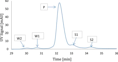
The peptide of interest is a 3.4 kDa peptide with a pI of 9.3. This polypeptide is used for treatment of osteoporosis, Paget’s disease and chronic pain in terminal cancer patients. In this work, we have taken raw polypeptide mixture in powder form directly from the industrial production process, so that a real industrial multi-component system can be evaluated. This raw powder was mixed with buffer A1 to make it suitable feed for the system. In order to simplify the purification problem, the polypeptide mixture is divided into five key components. These components are divided into their categories based on chromatogram shown in Figure 2.1. Classification of impurities is done based on their elution timing and position. Only impurities which are close to peptide peak are considered because these impurities present the highest difficulty in separation process. As mentioned

earlier in introduction chapter, W1 and W2 represents the weak impurities, P

denotes peptide and S1 and S2 indicates groups of strong impurities. The ﬁnal

system is made of these ﬁve key components.

0 10 20 30 40 50 60 29 30 31 32 33 34 35 36 U V S ig na l [ m A U ] Time [min] W2 W1 P S1 S2

Figure 2.1: Analytical chromatogram (UV = 280nm) of the polypeptide mixture with the nomenclature of peptide and impurities. Only impurities very close to peptide are considered as they are most diﬃcult to separate.

(16)

2.2.2 Chemicals

HPLC grade acetonitrile is used as organic modiﬁer. Sodium dihydrogen phos-phate, orthophosphoric acid are used to make buﬀer for desired concentration of

H3P O4. Triﬂuoroacetic acid (TFA) is used alone as a buﬀering agent. Whereas

acetic acid(AcOH) and sodium acetate(AcONa) are used for desired concentrations of AcOH. Milipore de-ionized water is used for making buﬀers. All respective buﬀer compositions are listed in Table 2.1.

Buﬀer Composition A1 20mM-160mM NaH2P O4 at pH 3.25 in AcN/H2O 3/97 (v/v) B1 20mM-160mM NaH2P O4 at pH 3.25 in AcN/H2O 50/50 (v/v) A2 20mM H3P O4 at pH 3.25 in AcN/H2O 6/94 (v/v) B2 20mM H3P O4 at pH 3.25 in AcN/H2O 50/50 (v/v) A3 10mM TFA in AcN/H2O 6/94 (v/v) B3 40mM TFA in AcN/H2O 50/50 (v/v) A4 100mM AcOH in AcN/H2O 2/98 (v/v) B4 800mM AcOH in AcN/H2O 50/50 (v/v)

Table 2.1: Composition of All Buﬀer Solutions

2.2.3 Chromatography Equipment and Columns

The experiments are carried out on Agilent 1100 Series HPLC, equipped with a quaternary gradient pump, an auto-sampler, an online degasser, and a temperate two column switch, a diode array detector and a refractive index detector. A Gilson FC203B fractions collector is used to collect fraction from column outlet. pH measurement is done by Mettler Toledo pH sensor. Experiments in diluted and overloaded conditions are performed on Kromasil 100-10-C18 column of length 250 mm and 4.6 mm diameter. This column is packed with silica based reverse phase material. Mean particle size of the column is 10µm and column has a pore size of 100 Å. For analysis of purity of peptide fractions collected during overloaded experiments, a Waters symmetry shield RP 8 100Å, 3.5µm, 4.6 mm X 50 mm column is used. This is a reverse phase column which is basically used for analytical chromatography.

(17)

2.3 Methods

In this section of this chapter we explain the experimental and mathematical pro-cedures to determine the model parameters. Overall Henry coeﬃcients and column porosity are evaluated with retention time of components measured in diluted con-ditions. Characteristics equation can be used to calculate these parameters from retention time. Mass transfer constants are calculated from stoichiometric equa-tions in literature. Rest of the model parameters are regressed from experiments in overloaded conditions at diﬀerent counter-ion concentration.

2.3.1 Characteristics Equation

To characterize the components behavior in diluted condition, ideal case model Equation (2.3) is used. Using method of characteristics a solution for ideal model equations can be written as:

∂t ∂x = 1 + φi ∂q ∂c ulin (2.13)

This equation defines characteristics at specific concentration. Linear isotherm can be assumed for experiments in diluted conditions, as defined in Equation (2.4). Substituting Equation (2.4) into Equation (2.3), we get the following equations:

∂t

∂x =

1 + φiHi

ulin (2.14)

Integrating both side we get, ? tR,i 0 ∂t = ? L 0 1 + φiHi ulin ∂x (2.15)

In diluted conditions Henry coeﬃcient (H) is constant along the column, tR,i =

L ulin

(1 + φiHi) (2.16)

Where tR is the retention time, L is the column length and φ = (1 − ?i)/?i is the

phase ratio.

2.3.2 Column Porosity

Accessible column porosity of peptide is an important parameter of adsorption model and it is calculated experimentally. Porosity accessible to component i is

(18)

deﬁned as:

?i =

VL,i

Vc (2.17)

Where Vc is the column volume and VL,i is the column volume available to speciﬁc

peptide. Porosity is evaluated with the experiments in diluted conditions. Isocratic experiments with small volume injection of peptide mixture are performed on Kromasil C18 column. Mobile phase composition of 100 % buﬀer B1 is used for peptide elution. At very high acetonitrile concentration, the peptide does not adsorb onto stationary phase [13] and elutes very fast. This implies that the peptide retention times is similar to column dead time for the peptide, t0,i. Thus,

porosity accessible to the particular pepide can be calculated by from Equation (2.16) as: Hi = 0, tR,i = L ulin = t0,i = L?i usup (2.18) ?i = Q.t0,i Vc (2.19)

Where usupis the superﬁcial velocity and Q is the ﬂowrate into column. Moreover,

there is also a an HPLC dead time which is deﬁned as the time taken for injection to travel through all tubing and instruments other than the column. This dead time must be subtracted from the column dead time to measure available porosity.

2.3.3 Henry Coeﬃcients

Henry coeﬃcients are also measured with experiments in isocratic diluted condi-tions. Henry constants of component i can be calculated from equation (2.16):

Hi = ? tR,i t0,i − 1 ? ? φi (2.20)

These experiments of small volume injections are performed at different counter-ion concentrations. At each counter-ion concentration, different constant acetonitrile concentrations are use to measure the value of Henry constants. The measured values of Henry constants of polypeptide and impurities at constant counter-ion compositions are shown in section (2.4). The final obtained values are fitted to stoichiometric displacement model as defined by Equation (2.8). All corresponding fitting values are reported in section (2.4). From this data of Henry constant, selectivity of impurities can then be calculated:

S = Hi

(19)

Where S is the Selectivity, Hi and Hp are the Henry constants of impurities and

peptide. Selectivity is used to quantify the separation process for respective im-purities.

2.3.4 Preparative Experiments

In industrial preparative chromatography higher amounts of loading are used on columns to get higher productivity. Therefore, it is very crucial that adsorption model in our case should have very good predictions in overloaded conditions. Henceforth, a series of overloaded experiments were carried out. At each counter-ion concentratcounter-ion three diﬀerent acetonitrile gradients are used. 5g, 10g and 15g of peptide per liter of column volume is used for respective acetonitrile gradients. Loading time is calculated in each case to perform these preparative experiments:

tload = Vload Qload = mlaod Ccrude × Qload = Vc× mvol Ccrude× Qload (2.22)

Where tload is the loading time, Ccrude is the concentration of peptide in feed

mixture, Qload is the volumetric ﬂow rate, Vload is the volume of peptide loaded,

mload is the mass of peptide loaded and mvol represents the mass of peptide loaded

per unit volume of column. Overloaded experiments are carried out on Kromasil C18 column with the following procedure:

1. Equilibrium of column at low modiﬁer concentration (100% buﬀer A1) for 3-4 column volumes

2. Loading of petide onto column with tload

3. Washing at lows modiﬁer concentration (100% buﬀer A1) for 3-4 column volumes

4. Gradient of Modiﬁer concentration, (elution occurs)

5. Washing with high modiﬁer concentration (100% buﬀer B1) for 3-4 column volumes

UV absorbance length is set at 310nm. During step of modifier gradient, fractions are collected at the end the column. A total of 9 preparative experiments are performed. The fractions are analyzed on symmetry shield RP8 column. Buffer A2 and buffer B2 are used in this analytical procedure. The analytical experiments are done by following method:

(20)

1. Equilibrium of column at modiﬁer composition of 15% buﬀer B2 and 85% A2 for 3-4 column volumes

2. Gradient of Modiﬁer concentration from 15% B2 to 55% B2 in 30 min-utes(elution occurs)

3. Washing with high modiﬁer concentration of 100% buﬀer B2 for 3-4 column volumes

In this procedure, UV absorbance length is set at 220nm. The injection amount of each vial fraction depends up on the concentration of component in that vial. An estimation of the injection volume is performed so that we can obtain all component peaks in the range of 500 to 700 mAU (milli-adsorbance units). The purity of speciﬁc component in each vial is calculated by taking ratio of that area under that component peak by sum of areas under all peaks. Concentration and mass of the particular component in each vial is the calculated from following equations:

Ci =

Q_{× A}p,i

Vi× UVcal (2.23)

mi = Ci× Vi (2.24)

Where Ci is the concentration of compound in vial i, Ap,i is the area under that

component peak in vial i, Vi is the injection volume, mi is the concentration

of compound in vial i and UVcal is the UV calibration factor for that speciﬁc

component. This procedure is followed for analysis of polypeptide and impurities in all selected vials. The impurities found in each vial are lumped together with respect to their selectivities on analytical column. Each lump is then treated as a individual impurity. Impurities are classiﬁed with a selectivity less than 0.9 as W2 and between selectivity of 0.9 and 1 as W1. Lump of impurities from selectivity of 1 to 1.15 is called S1 and impurities of selectivity greater than 1.15 are named as S2. W1 and W2 are known as weak impurities whereas S1 and S2 are called strong impurities. This grouping of impurities is shown in a typical analytical chromatogram in Figure 2.1.

It is very important to validate the above described experimental technique. Therefore mass balance across the column is calculated. Mass of the peptide, injected into column, is compared with the summation of outlet mass of peptide in all fractions for that speciﬁc preparative experiment, as shown in Equation (2.25).

M B = mrecoup

(21)

Where MB is ratio of total recovered mass, mrecoup to the mass loaded into column,

mload. Ideally mass balance should be equal to 1. If MB is not equal to 1, then there

might be some problem associated with experimental procedure, measurement techniques and calculations. In this thesis work, mass balance of all preparative experiments is in the range of 0.99 to 1.05.

Purity, yield and productivity are main evaluation parameters for a production process. After validating experiments with mass balance, purity of peptide in each fraction is calculated. Yield for that speciﬁc purity constraint can be measured with Equation (2.26).

Y = mp,out

mload (2.26)

Where mp,out is the total mass of peptide in fractions of speciﬁed purity, Y is yield

with respect to mass recuperated. The productivity of the preparative experiment is deﬁned as:

P = Y × mload

Vc× trun (2.27)

Where P is productivity and trun is the time in which speciﬁc experiment will be

completed.

2.4 Parameters

2.4.1 Porosity

The available column porosity plays an important role in deﬁning the column be-havior. The porosity is calculated by measuring retention times in non-adsorbing conditons as described in section (2.2.3). The dead time for HPLC is found to be 0.09 min. The retention time of small peptide injections is measured at

dif-ferent counter-ion, H3P O4 concentrations of 20mM, 50mM, 100mM, 150mM and

165mM. The ﬁnal results are shown in Figure 2.2. It is observed the porosity

increases with the increase in H3P O4 concentration, reaches a maximum and then

decreases on increasing counter-ion concentration. This phenomena is also ob-served in previous studies by Getaz et al. [13]. It is believed that increase in porosity with the counter-ion concentration is due to electrostatic eﬀects on re-vere phase material. Peptide is positively charged at low pH conditions. With

the increase in ionic strength, more peptide charges can be shielded by H3P O4,

which results an increase in porosity. However, at higher ionic concentration, there

(22)

0.36 0.38 0.4 0 0.05 0.1 0.15 0.2 Pe pt id e Po ro si ty [ -]

Ionic Strength (Molar)

Figure 2.2: Available column porosity for polypeptide and impurities. The ﬁlled squares represents the experimentally measured values, whereas line represents the ﬁtting

eﬀect of complex formation, apparent size of peptide molecules starts increasing. Therefore, the porosity starts decreasing after a certain counter-ion concentration. Experimental values of peptide porosity are ﬁtted with a quadratic function of counter-ion concentration:

?(CH3P O4) = p1C

2

H3P O4 + p2CH3P O4+ ?min (2.28)

Where p1 and p2 are the ﬁtting parameters with values of -3.4016 and 0.5712

respectively. Coeﬃcient of determination, R2 _{of this model is 0.94. ?}

min can be

quantiﬁed as porosity when analyte concentration is zero. The ?min for Kromasil

c18 is found to be 0.3657. This is comparable with respect to the porosity reported in earlier studies on this column [13].

2.4.2 Henry Coeﬃcient

Overall Henry coefficients of the polypeptide and the main impurities are calcu-lated as a function of acetonitrile concentration at counter-ion concentrations of 20mM, 50mM, 100mM, 150mM and 165mM. Henry constants are fitted as a func-tion of acetonitrile concentrafunc-tion. Linear solvent strength model is used as defined in equation (2.8). Figure 2.3 shows the Henry constants of polypeptide at specified counter-ion concentration. Henry constants of impurities are shown in Appendix A. Our goal in this section is to provide such a model that deals with effects of variations in counter-ion concentrations together with acetonitrile concentrations.

(23)

0 0.5 1 1.5 2 26 28 30 32 Lo g H [-] ACN [v/v] Ionic Strength = 50mM 0 0.5 1 1.5 27 28 29 30 31 32 Lo g H [-] ACN [v/v] Ionic Strength = 100mM 0 0.5 1 1.5 2 26 27 28 29 30 31 Lo g H [-] ACN [v/v] Ionic Strength = 165mM 0 0.5 1 1.5 26 27 28 29 30 31 32 Lo g H [-] ACN [v/v] Ionic Strength = 20mM 0 0.5 1 1.5 27 28 29 30 31 32 Lo g H [-] ACN [v/v] Ionic Strength = 150mM

Figure 2.3: Henry Coefficients of polypeptide as a function of Acetonitrile concen-trations at different counter-ion concenconcen-trations. Blue filled squares are the experi-mentally measured values, whereas lines represents the corresponding fitting with linear solvent strength model.

(24)

The effects of ionic strength on Henry constants at constant acetonitrile concen-trations is shown in Figure 2.4. The Henry coefficient of peptide and impurities increases up to certain counter-ion concentration to attain a maximum and the decreases with increase in counter-ion concentration. The increase and decrease of the Henry coefficient is in agreement with the previous studies [11]. This phe-nomena can be expalined by the forces involved in reverse phase chromatography : (a) the attractive force between a compound and the stationary phase. (b) the electrostatic forces between charged molecules. The counter-ion concentration in buffers effect these forces. It can be explained with three different mechanisms [15] 1. Classical-pairing effect: forming of a neutral complex between counter-ion

and peptide enhances the peptide retention.

2. Chaotropic eﬀect: the disruption of salvation shell of the peptide by counter-ion, which can lead to an increase in apparent hydrophobicity of peptide, consequently increases retention.

3. Lipophilic eﬀects: adsorption of counter-ion on the surface of stationary phase, thus creating additional attractive forces between peptide and sta-tionary phase.

An increase in counter-ion would therefore cause an increase in retention time by increasing attractive forces (Chaotropic effect, Lipophilic effect) and decreas-ing repulsive forces (ion-pairdecreas-ing). In case of H3P O4 counter-ion, after a specific

counter-ion concentration ion-pairing phenomena starts dominating as described in previous section. Therefore there is a parabolic proﬁle is observed in case of phosphate counter-ion as observed by Getaz et al. [11]. The kinetics of this phe-nomena can be explained by classical stoichiometric model [14]. A relationship can be found between counter-ion concentration, acetonitrile concentration and Henry constant as follows:

H = HA + HACK[CH3P O4] 1 + K[CH3P O4]

(2.29) log(HA) = log(HA,W) + mA,AcNCAcN + mA,H3P O4CH3P O4 (2.30) log(HAC) = log(HAC,W) + mAC,AcNCAcN + mAC,H3P O4CH3P O4 (2.31)

Where HA and HAC are the Henry constants in pure water of the analyte and the

analyte-counter-ion respectively. mA,AcN, mA,H3P O4, mAC,AcN and mAC,H3P O4 are the fitting coefficients. Fitting of Equation (2.29) is shown in Figure 2.4 and fitted model values are summarized in Table 2.2.

(25)

20 40 60 80 100 120 140 160 180 5 10 15 20 25 30 35

Sa lt C onc entra tion (C_{Sa lt})(mM)

H en ry C o ffi ci en t C_ACN = 27.2 C_ACN = 27.5 C_ACN = 27.9 C_ACN = 28.4 C_ACN = 29 Fitting

Figure 2.4: Henry coefficients of polypeptide as a function of counter-ion concen-tration at different constant acetonitrile concenconcen-trations. Empty squares are Henry constant values that are calculated from fitting equations of linear solvent strength models at respective counter-ion concentrations. Curved lines represents the fitting

of Henry coeﬃcients as shown in Equation (2.29). R2 _{of this ﬁtting is 0.9814.}

Component HA,W mA,AcN mA,H3P O4 HAC,W mAC,AcN mAC,H3P O4 K

W2 1.831 -1.9255 0.0294 11.747 -0.3148 -0.0050 0.00048

W1 1.131 -1.6255 0.0294 11.4391 -0.2999 -0.0053 0.00048

P 1.131 -1.6255 0.0294 11.181 -0.2868 -0.0055 0.00048

S1 7.1433 -0.2242 -0.0049 10.2193 -0.2519 -0.0049 0.00048 S2 7.1433 -0.2242 -0.0049 10.3193 -0.2519 -0.0050 0.00048

(26)

2.4.3 Mass Transport

Mass transfer coeﬃcient km and dispersion coeﬃcient Dax are very important

pa-rameters to define physics on interface. Mass transfer resistance in adsorption phenomena can be divided [2] into: (a) fluid phase surrounding particle, (b) pore diffusion, (c) adsorption at liquid - solid interface and (d) solid or adsorbed phase diffusion. In this work mass transfer resistance is lumped into single resistance parameter, and it is assumed that pore diffusion dominates the overall mass transfer for adsorption. Henceforth, mass transtransfer coefficient is calculated by Stokes -Einstein diffusion equation. Moreover in case of reverse phase chromatography, diffusion process depends upon the ion concentration. At higher counter-ion concentratcounter-ions, peptide make larger complex compounds with counter-counter-ion, which makes them more difficult for diffusion. This situation can not be described by Stokes-Einstein equation alone. Accordingly, diffusional hindrance correction factor is applied to Stokes-Einstein equation and is shown in Equation (2.32).

Dp = ? kBT 6πµrpeptide ? ? ? ? + 1.5(1_{− ?)} ? ? 1 + 9 8λlnλ− 1.54λ ? (2.32) km = 15Dp Hr2 p , where λ = rpeptide rpore (2.33)

Where kB is the Boltzmann constant, µ is the mobile phase viscosity, H is the

Henry coeﬃcient, T is the process temperature, rpeptide is the radius of the peptide,

rpore is the radius of the pores and rp is the radius of the particles of stationary

phase. In Equation (2.32) ﬁrst part is the Stokes-Einstein equation and middle term handles the change in porosity. Last term is known as Brenner-Gaydos correction factor and accounts for obstructions in diﬀusion of peptide molecules

into pores. Additionally, the dispersion coeﬃcient Dax is calculated with mass

transfer correlation [2]: Dax = dpv 0.2 + 0.011Re0.48, where Re = ρvdp µ (2.34)

Where dp = 2rp is the diameter of stationary bed particle, Re is the Reynolds

number and ρ is the density of mobile phase. Values of the all parameters of Equations (2.32), (2.33) and (2.34) are displayed in Table 2.3.

2.4.4 Saturation Capacity

Saturation capacity is the maximum amount of a component that can be adsorbed onto stationary phase. In our adsorption model we have assumed two sites for ad-sorption with saturation capacities of qsat,1,iand qsat,2,i. These saturation capacities

(27)

Parameter Value Units kB 1.3806488× 10−23 m2kgs−2K−1 T 25 ◦_C µ 0.0008 Kg/(sec.m) rP eptide 1.57× 10−9 m ρ 900 Kg/m3 km 415.6957 1/min Dax 4.9825× 10−8 m2/sec

Table 2.3: Mass transport parameters

are further related to Henry constants of respective adsorption sites. In previous subsection, we have shown the procedure to determine the overall Henry coeffi-cients, however for estimation of Henry coefficients H1,i and H2,i, first we have to

evaluate coeﬃcients involved in these relations. In this study inverse method is used to regress these parameters.

Once the dependence of the Henry coefficients is established by the diluted experiments, overloaded linear gradient elution experiments are performed to fix the dependence of the saturation capacity on the ionic strength. The detailed procedure for experiments and the separation process in overloaded conditions has been described described above in section (2.3.4). The mixture was loaded on a single preparative column and eluted with application of linear gradient of modifier concentration. The elution was fractionated (1 mL per fraction) and each fraction analyzed for concentrations of peptide and impurities. The gradient elution condi-tions are described in Table 2.4. Counter-ion concentracondi-tions, 50mM, 100mM and 150mM are selected for preparative experiments to find the parameters as a func-tion of counter-ion concentrafunc-tion. For each salt concentrafunc-tion three overloaded experiments are performed at different acetonitrile gradients and shown in Ta-ble 2.4. Modifier gradient elution is carried out from 0% buffer B1 to 100% buffer B1 in 30 min and 60 min for each case. However, third modifier gradient elution was performed at optimized elution time in diluted conditions as shown in Fig-ure 3.2. These gradient times are obtained from maximum selectivity conditions in diluted conditions.

(28)

Counter-ion concentration [mM] AcN gradient time [min] Loading [g/L] Slope [v/v AcN/min] 30 5 1.566 50mM 44 15 1.068 60 10 0.783 30 5 1.566 100mM 40 10 1.175 60 16 0.783 30 10 1.566 150mM 36 5 1.305 60 20 0.783

Table 2.4: Experimental conditions of preparative experiments

A typical chromatograms of overloaded experiments is shown in Figure 2.5. The analyzed fractions shows some pure regions for peptide, although many fractions are the mixtures of two or more components. The basic aim of the chromatographic separation process is to elute the pure fractions of the peptide in the corresponding chromatogram. Additionally along with peptide, we can also see the elution proﬁles of impurities. All preparative elution proﬁles are displayed in Appendix B.

(29)

0 5 10 15 20 25 30 35 40 45 50 0 5 10 15 20 25 30 25 30 35 40 45 50 Co nc en tr at io n [g /L ] Time [min] UV signal [v%] L1 [g/L] H1 [g/L] H2 [g/L] Peptide [g/L] L2 [g/L] AcN [v/v] A CN (v /v )

Figure 2.5: Example of Preparative experiment. The loading of this experiments was 16 g/L, gradient time of acetonitrile was from 0%B1(buﬀer) to 100%B1(buﬀer)

in 60 min and concentration of H3P O4 is 100mM. The black line represents the

UV signal from preparative experiment at 310 nm, whereas the dashed line shows acetonitrile concentration. Markers in the plot are the concentration of peptide and impurities. Correspondingly marker depictions are shown on right side of the chromatogram.

(30)

Chapter 3 Mathematical Modeling and

Optimization

The results of the previous chapter have enlightened the complex behavior of porosity and Henry constants with the counter-ion concentration. In addition to that, preparative elution profiles were presented at different counter-ion concen-trations. Now we need to calculate saturation capacities for complete description of the lumped kinetic model. There are many variables involved into adsorp-tion isotherm. Experimental measurement of parameters would consume a large amount of polypeptide mixture and it is very difficult to complete these experi-ments in the given time frame of the master thesis. Furthermore, the nature of the adsorption isotherm and the variations in parameters makes the system extremely sensitive to small errors in the parameters. Therefore, the model parameters are directly regressed using numerical modeling techniques. In the first part of this chapter, computational modeling of the elution profiles is presented for the com-plete characterization of the adsorption model.

Moreover, the aim of this chapter is not only to calculate the relevant model parameters, but to use the model as an instrument for the understanding and optimization of the adsorption process in case of single and double gradient elution techniques. Therefore, variation in model parameters is described as a function of counter-ion concentration. Second part of this chapter illustrate the validation of our adsorption model. It is also explained in this chapter that our model is not only able to calculate yield and productivity in a good comparison with experimental data, but it can easily deal with the complex double gradient elution techniques. After model calibration and validation by comparison with suitable experimental data, Pareto optimizations of the process were carried out at diﬀerent counter-ion

(31)

concentrations and double gradient. Final part of this chapter shows the modeling and implementation of the optimization techniques with the analysis of the results from single and double gradient methods.

3.1 Computational Modeling

After completing all overloaded experiments in chapter 2, isotherm parameter are regressed by using peak fitting methods. As we know that there is no analytical so-lution for the lumped kinetic model. Numerical methods are implemented to solve adsorption model with MATLAB and FORTRAN. To solve the chromatographic mass-balance equations, methods like finite difference and orthogonal collocation have been used in the literature[10]. Finite difference method is easy to imple-ment and give satisfactory results. Therefore, differential equations are solved with method of lines, which is based on finite difference method.

3.1.1 Method of Lines

The chromatographic mass balance equations are a set of partial differential equa-tions. In this method, space derivatives are converted in difference equations over a small discretization interval. Equations (3.1) and (3.2) are discretized with cen-tral difference and backward difference methods. In this way all partial differential equations are converted into ordinary differential equations. Grid for position in space x is shown in Figure 3.1. On right hand side an extra point is added to demonstrate the boundary conditions.

∂c ∂t = DL ∂2_c ∂x2 − ulin ∂c ∂x − (1_{− ?)} ? ∂q ∂t (3.1) ∂q ∂t = kM(qeq− q) (3.2)

The Initial and boundary conditions for the set of partial diﬀerential equations are:

Initial Condition:

t = 0, c = 0, q = 0, qeq= 0 (3.3)

Danckwerts and Neumann boundary conditions are used to deﬁne the mass balance at inlet and outlet of chromatographic column.

At x = 0

DL

∂c(t, 1)

(32)

?

ℎ

_?

0 ?

0

?

1

?

2

?

k-1

?

k

?

k+1

?

N-1

?

1

N

?

N+1 Figure 3.1: Grid for descretisation in space x

At x = L

∂c

∂t = 0 (3.5)

Feed conditions are deﬁned as:

x = 0, cin(t) = cf,i when t≤ tf

x = 0, cin(t) = 0 when t > tf

(3.6) (3.7) Here xk = k× hx, k = 1, 2..., N-1, N and hx = L/(N − 1). N is the number of

grid points.

Substituting ∂q

∂t and descretize equation for point k at time t is written as:

dck dt = DL ?ck+1− 2ck+ ck−1 h2 x ? − ulin ?ck+1− ck hx ? −?1 − ? ? ? kM(qeq,k− qk) dqk dt = kM(qeq,k− qk) (3.8) (3.9) In diluted conditions qeq,k is calculated with the linear isotherm.

qeq,k = Hkck (3.10)

qeq,k is measured with bi-Langmuir isotherm in case of overloaded conditions.

qeq,k = ckH1,k 1 + ncomp? j=1 ? ck,j_q_sat,1,jH1,j ? + ckH2,k 1 + ncomp? j=1 ? ck,j_q_sat,2,jH2,j ? (3.11)

Where qsat,1,j and qsat,2,j are given by Eq. (2.12). Discretized Equation (3.8) at

boundary condition of k = 1 is written as: ∂c1 ∂t = DL ?c2− c1 h2 x ? − ulin ?c1− cin hx ? −?1 − ? ? ? kM(qeq,1− q1) (3.12)

(33)

At k = N, applying Neumann boundary conditions, Equation (3.8) is describes as: dcN dt = DL ?cN−1− cN h2 x ? − ulin ?cN − cN−1 hx ? −?1 − ? ? ? kM(qeq,N − qN) (3.13)

Equations (3.8) to (3.13) form a system of linear ODEs at a speciﬁc time (t).

A(t, c)_{× c}? = B(t, c) (3.14)

where c is the vector of the unknown functions i.e. concentrations , c? _{is the time}

derivatives,A and B are the the matrices of the coefficients. In this thesis Netlib FORTRAN solvers are used. The numerical code has been written in Fortran-95 and the system of ODEs solved using the DLSODE package. The simulations were run on a Intel Xeon 6 core processor. In diluted conditions, method of lines is used to find the acetonitrile gradient conditions to maximize the selectivity of impurities. A single objective function is defined as the ratio of selectivity of weak impurity to strong impurities which are closest to peptide. This ratio if directly proportional to the retention times of components in the simulated elution profiles. MATLAB inbuilt optimizers as Genetic Algorithm (GA) and FMINCON are used to find the minimum of the objective function. Correspondingly results are shown in Figure 3.2.

(34)

0.93 0.94 0.95 0.96 0.97 35 37 39 41 43 45 0 50 100 150 200 O p ti m iz ed R at io o f Se le ct iv it y[ -] A cN G ra d ie n T im e [M in ] Couter-ion Concentration [mM] AcN Gradient Selectivity Ratio

Figure 3.2: Results from optimization with respect to counter-ion concentrations. Filled red circles represents the optimized ratio of selectivity, whereas ﬁlled blue squares are the corresponding acetonitrile gradient times. Lines represents the normal ﬁtting of the pointed values.

3.1.2 Parameters Regression

The non-linear region of the adsorption isotherm, that is the saturation capacity, is regressed by simulating overloaded linear gradient elution experiments. Method of lines is implemented to calculate outlet concentration profiles at the same over-loaded conditions as described in Table 2.4. The difference between experimentally measured outlet concentration and the simulated profiles is minimized. The ge-netic algorithm (GA) package of the MATLAB is use to find the global minimum of the objective function. In this procedure lower and upper limits of the isotherm parameters are assigned to the solver. In order to simplify the regression proce-dure, the simulations were designed in such a way that the possible least number of parameters vary with the counter-ion concentration. The rationale behind the proposed regression procedure will be discussed later in this report. The values of the Henry constants, porosity and mass transfer constants are conveyed from previous chapter. It is assumed that the saturation capacities of polypeptide and other impurities are same.

(35)

Ionic Strength[mM] α1 α2 α3 α4 α5 α6

50 0.8742 0.4711 0.0001 20.6732 361.7080 142.0675

100 0.6173 0.5741 0.0001 20.6732 361.7080 142.0675

150 0.5552 0.7044 0.0001 20.6732 361.7080 142.0675

Table 3.1: Isotherm ﬁtting parameters for polypeptide and impurities at respective counter-ion concentrations

At ﬁrst, adsorption model parameters are estimated for ionic strength of 50mM. Regression procedure is carried out simultaneously with all three overloaded exper-iment of 50mM. For further calculations at 100mM and 150mM, regressed

parame-ters of 50mM are kept constant except α1 and α2. Consequently these parameters

are evaluated at respective ionic strengths. In this manner we are successfully able to measure the model parameters such that variations of isotherm parameters is limited to two variables only. A reduction of the set of estimated parameters also leads to better conditioning of the parameter estimation problem and reduces the numerical eﬀorts. It also helps in improvement of convergence and robustness of the numerical simulations. The results of the outlet concentration based on regressed model parameters are shown in Figure 3.4, whereas the values of the regressed parameters for describing qsat,1 and qsat,2 of the peptide (see Eq. (2.12))

are reported in Table 3.1.

As we can see from Figure 3.4 that overall quality of the peak ﬁtting is good.

Based on R2

f it value it can be noticed that there is a very good similarity between

simulated and experimental outlet concentration proﬁles. The elution proﬁles of impurities are estimated with a good resemblance with experimental data. To this regard, it must be pointed out that the quality of the overloaded experiments and simulation techniques was particularly good. Additionally, it can be observed

that the elution proﬁle of strong impurity H2 does not show a good resemblance

to experimental data. This behavior can be explained with displacement eﬀect of impurities. As the loading volume of polypeptide mixture increases, the amount of column space required by the impurities and peptide also increases. Therefore, due to interactions between impurities and peptide, a displacement of the peak occurs in the column. As a result; the numerical prediction of the outlet concentration proﬁle of strong impurity H2 is not ideally identical to the experimental data.

(36)

18 20 22 24 26 28 10 20 Time [min] C on ce nt ra tio n [g /L ] 18 20 22 24 26 280 200 400

G radient time = 30 min, Loading = 5.0018g/L of c olumn,

A C N C on ce nt ra tio n [g /L ]

(a) Ionic Strength = 50mM, R2

f it = 0.94 22 24 26 28 30 32 34 10 20 Time [min] C on ce nt ra tio n [g /L ] 22 24 26 28 30 32 34 0 100 200 300 400

G radient time = 44 Min & Loading = 15 g/L

A C N C on ce nt ra tio n [g /L ] (b) Ionic Strength = 50mM, R2 f it = 0.97 32 34 36 38 40 42 44 46 10 20 Time [min] C on ce nt ra tio n [g /L ] 32 34 36 38 40 42 44 460 100 200 300 400

G radient time = 60 Min, Loading = 10 g/L

A C N C on ce nt ra tio n [g /L ] (c) Ionic Strength = 50mM, R2 f it = 0.94 24 26 28 30 32 34 10 20 Time [min] C on ce nt ra tio n [g /L ] 24 26 28 30 32 340 500

A C N C on ce nt ra tio n [g /L ] (d) Ionic Strength = 100mM, R2 f it = 0.98 32 34 36 38 40 42 44 46 10 20 Time [min] C on ce nt ra tio n [g /L ] 32 34 36 38 40 42 44 460 100 200 300 400

(e) Ionic Strength = 100mM, R2

f it = 0.98 19 20 21 22 23 24 25 26 10 20 Time [min] C on ce nt ra tio n [g /L ] 19 20 21 22 23 24 25 260 200 400

A C N C on ce nt ra tio n [g /L ] (f) Ionic Strength = 150mM, R2 f it = 0.96

(37)

22 23 24 25 26 27 28 29 30 10 20 Time [min] C on ce nt ra tio n [g /L ] 22 23 24 25 26 27 28 29 300 200 400

(a) Ionic Strength = 150mM, R2

f it = 0.95 32 34 36 38 40 42 44 10 20 Time [min] C on ce nt ra tio n [g /L ] 32 34 36 38 40 42 44 0 200 400

A C N C on ce nt ra tio n [g /L ] (b) Ionic Strength = 150mM, R2 f it = 0.94

Figure 3.4: Results of peak ﬁtting of all preparative experiments at counter-ion concentration of 50mM, 100mM and 150mM. Symbols represents the experimental values, whereas solid lines are results of numerically calculated peaks with regresses model parameters. Red, green, blue, light blue and black markers and solid lines of the same colors represents W2, W1, Peptide, S1 and S2 respectively.

(38)

3.2 Model Validation

Validation is a set of methods to decide a model’s accuracy and quality for prospec-tive utilization. This information can be used to determine the results applicability in the process modeling and optimization. Validation is the only way to determine how well the model predict the relevant results. No matter how validations are done, there will inevitably be uncertainty about some aspects of a model. Therefore we have emphasized our validation on the most important results of the process i.e. yield and productivity. In the previous section we have successfully estimated all the parameters in the lumped kinetic model. The next part of this thesis fo-cuses on the process optimization. As we have already decided to perform a model based optimization, it is very important to authenticate the adsorption model. In this section, we establish the relationships between regressed parameters and the counter-ion concentrations. Experimental and numerical results of the yield and the productivity are compared for the veriﬁcation of the adsorption model.

3.2.1 Parameters Vs Counter-ion concentration

From model parameters shown in Table 3.1, it is observed that ﬁtting parameters

of equation for Henry coeﬃcients H2,i of second adsorption site are not constant

with the change in counter-ion concentrations. It is very important to define such a model that must account for the variation in parameters with ionic strength. Therefore least square fitting method was implemented in MATLAB to find a correlation between α1, α2 and ionic strength. From this we found:

α1 = 0.023CH3P O4 + 0.3499 (3.15)

α2 = 4× 10−5CH23P O4 − 0.011CH3P O4 + 1.3259 (3.16)

The values of α3 to α6 are independent of CH3P O4 as can be seen from Table 3.1. The presented correlations are only valid in experimental range. These equations

are plotted with the regressed parameters and shown in Figure 3.5 and 3.6. R2

f it

for the relevant model equations of α1 and α2 are 1 and 0.993. Henceforth, the

(39)

0.5 0.65 0.8 0.95 40 60 80 100 120 140 160 ? 1 Ionic Strength (mM )

Figure 3.5: Fitting parameter α1 vs Counter-ion concentration

0.43 0.58 0.73 40 60 80 100 120 140 160 Ionic Strength (mM) ? 2

Figure 3.6: Fitting parameter α2 vs Counter-ion concentration

3.2.2 Comparison of Numerical and Experimental Results

In this part of the report, numerically calculated yield and productivity are com-pared with experimental data for the adsorption process. The motivation is to validate the ultimate adsorption model. In particular we have to make sure that numerical prediction of yield and productivity are similar to experiments in over-loaded conditions. At ﬁrst we have calculated the yield and productivity for our preparative experiments as described in section (2.3.4). A purity constraint of 94% is applied in these calculations. The yield and productivity is then calculated from numerical simulations of the adsorption model with same experimental pro-cess parameters, reported in Table 2.4. Accordingly outlet concentration proﬁles of Figure 3.4 are divided into many fractions in a similar way of integration process.

(40)

0.4 0.6 0.8 1 1.2 1.4 0.4 0.5 0.6 0.7 0.8 0.9 1 1.1 1.2 1.3 1.4 Yield

Yield from Numeric a l Simula tions [ ]

Yi el d fr o m E xp er im en ts [ ]

Figure 3.7: Comparison of experimental and simulated results of yield from prepar-ative experiments. Filled blue squares represents the results, whereas green lines are drawn to shown the 95% conﬁdence interval.

In each fraction, mass of the peptide and impurities is calculated. Purity of the individual mass fraction is measured by taking ratio of mass of peptide to the to-tal mass the fraction. All fragments satisfying purity constraint of 94% are chosen for evaluation of yield and productivity. Consequently yield and productivity are determined by Equations (2.26) and (2.27).

The final obtained results are shown in Figures 3.7 and 3.8. It can be seen that our model predictions of yield and productivity are in very good agreement with experimental data. A straight line is drawn with 95% confidence interval to show the quality of the fitting. Although, it can be noticed that in some experiments similarity between numerical and experimental values of productivity is more pronounced than the yield. In spite of this, it is more interesting to observe that all results are in confidence interval of each plot. Therefore we can conclude that our adsorption model is able to capture the physics of the chromatography process and it can be used to perform further optimization.

(41)

0 0.05 0.1 0.15 0.2 0.25 0.3 0.35 0.4 0 0.05 0.1 0.15 0.2 0.25 0.3 0.35 0.4 Produc tivity

Produc tivity from Numeric a l Simula tions [mg /mL/min]

Pr o d uc tiv ity fr o m E xp er im en ts [m g /m L/ m in ]

Figure 3.8: Comparison of experimental and simulated results of productivity from preparative experiments. Filled blue squares represents the results, whereas green lines are drawn to shown the 95% conﬁdence interval.

3.3 Model based optimization

The purpose of the model based optimization is to calculate the operating param-eters which gives the maximum purification efficiency and minimum separation costs while satisfying the product purity requirements. In this section, the vali-dated adsorption model is used to evaluate the separation efficiency of chromato-graphic process at different process conditions. This is a challenging task since our chromatographic model exhibit a strong non-linear behavior and only the elu-tion profiles at some process parameters can be quantified with the experimental efforts.

In industrial chromatographic purification process, there are many different parameters that should be optimized, such as purity, yield, buffers composition, productivity and product concentration. As we know that purity is the most im-portant criterion, whereas yield and productivity are the parameters which dom-inates the economy of the production process. Our main aim of this section is to find the optimum process conditions which gives the maximum profit. There are a quite of many factors which effects the industrial chromatographic process. These effects of process conditions are also related to each other. Now if we try to optimize individual process parameters then it would be very difficult and time

(42)

consuming to find the optimized values of each parameter. Henceforth, we have implemented multi-objective optimization techniques to find the optimum process conditions that gives the maximum yield and productivity. Finally Pareto fronts are use to analyze the separation efficiency of the chromatographic process at optimized process parameters.

3.3.1 Multiobjective Optimization

Multi-objective optimization is a mathematical formulation where two or more ob-jective functions are to be optimized simultaneously. Multi-obob-jective optimization is applied where optimal decisions need to be taken in the presence of trade-offs between two or more conflicting objectives. In charomatography, our main aim is to get the highest purity of the target component. Therefore the purity, which is the qualification of the product for putting into market, is to be defined as a primary constraint. Furthermore we always try to maximize the production of the target component to maximize our profit. All these criteria lead to identifying at least two objectives of the optimization studies:

1. The productivity, which is a count of the eﬃciency of the production unit and should be maximized

2. The product recovery or the yield, which should be maximized to increase earnings.

Although solvent consumption is also an important parameter in the production process, but it is not counted as an separate parameter because maximizing pro-ductivity insures least solvent consumption. The yield and propro-ductivity are deﬁned in Equations (2.26) and (2.27). These objective function are set to be maximized. In this work, MATLAB routines are implemented for multi-objective optimization [3]. As we know that these optimization routines try to ﬁnd the parameters for the minimization of the objective functions. Therefore, negative of the yield and productivity are taken as the ultimate objective functions.

The next step in this section is to deﬁne the process variables to be varied, i.e. process variable subjected to optimization. In our case following design variable are taken into account:

1. Solvent composition: Composition of the mobile phase is controlled by ap-propriate mixing of two diﬀerent concentration solvent. With the change in the concentration of the mobile phase, we can alter the interactions of the

(43)

polypeptide and impurities with the stationary phase. The mobile phase sol-vent plays a very important role in deﬁning the thermodynamic properties of the adsorption. In our model, Henry’s constant, porosity and saturation capacity have been expressed as functions of the mobile phase composition. Hence, modiﬁer and counter-ion concentration are considered as one of the design parameters.

2. Loading of polypeptide mixture: The concentration of the peptide feed mix-ture and volumetric ﬂow rate are kept constant at 5.6 g/L and 1 mL/min.

Variations in loading amount is deﬁned in terms of loading time (tload) or

time required for injection of feed solution into chromatographic column. A

lower and upper limit for tload is deﬁned in a way that the optimizer would

include the industrial loading conditions.

3. Cycle time: It has been already described that the cycle time depends upon loading and gradient time. We have already taken loading time as an individ-ual process variable, therefore gradient time tgrad is considered as a separate

design parameter. We have restricted the maximum gradient time up to 60 min to obtain a minimum productivity in every case.

Constraints on these parameters are listed in Table 3.2. At first we have calculated the Pareto fronts for the linear gradients of modifier concentration at constant ionic strength of 50mM, 100mM and 150mM. Four design parameters are selected, as loading time tload, the modifier gradient duration tgrad,1, the initial and final

ace-tonitrile concentration values of CAcN,ini and CAcN,f inal. A purity constraint of

94% of target polypeptide is applied. After optimization of this case, a Pareto front is calculated for simultaneous double gradient of counter-ion concentration and modiﬁer concentration. For an additional linear gradient of counter-ion con-centration three more design parameters are taken into multi-objective MATLAB routines: the counter-ion concentration gradient duration tgrad,2, initial counter-ion

(44)

Parameter Lower Bound Upper Bound Unit tload 3 15 min CAcN,ini 3 50 v/v CAcN,f inal 3 50 v/v CH3P O4,ini 50 150 mM CH3P O4,f inal 50 150 mM tgrad,1 0 60 min tgrad,2 0 60 min

Table 3.2: Constraints parameters for parameters of model based optimization

3.3.2 Results and Discussion

The optimum Pareto results from multi-objective optimization are displayed in Figure 3.9 and 3.10. It can be seen from the figures that the Pareto fronts are very well formulated and they are very efficient to demonstrate the optimum trade-off between the yield and the productivity. The maximum possible yield of approxi-mately 1.0 could be achieved at all process constraints, whereas it seems to be very difficult to obtain higher yield at counter-ion concentration of 50mM. As we have a relatively lower purity constraint, it can be noticed that comparatively higher yields are obtained in all Pareto fronts. Moreover it can be noted that maximum yield can be achieved at lowest productivity and opposite is also true.

Let us start the analysis of the results of these Pareto fronts for all design variables. The results of single gradient for all three counter-ion concentrations together with the results from double gradient are plotted in the same ﬁgure as shown in Figure 3.9. Pareto fronts of single gradient at constant ionic strength of 150mM and double gradient are presented in a separate Figure 3.10 to display the clear eﬀects of double gradient. Considering a constant gradient from Figure 3.9, it can be observed that the yield and the productivity have lowest values at counter-ion concentration of 50mM. The maximum values of the yield and the productivity are obtained at constant counter-ion concentration of 150mM. This is consistent with the optimized ratio of the selectivity (Sw/Ss) in dilute

conditions as shown in Figure 3.2. This implies that in all of the circumstances we should optimize the process parameters to maximize the selectivity of the strong impurities and minimize the selectivity of weak impurities. Saturation capacity does not eﬀect the adsorption in diluted conditions and we have established the relationship of Henry constant with modiﬁer concentration based on a theoretical and experimental basis. A general observation that can be noted from these results

(45)

is that higher selectivity ratio is deﬁnitely a better option in separation of the target polypeptide. It can also be noted that the selectivity has a direct impact on productivity as well.

It is observed that the yield and the productivity increases with the increase in concentration of H3P O4. To examine the reason behind the increase in

productiv-ity with the ionic strength, values of loading time are compared between the Pareto front parameters at respective counter-ion concentrations. Average loading time is calculated for each Pareto front of constant ionic strength. We have calculated loading times of 6.42min, 8.56min and 9.663min at counter-ion concentration of 50mM, 100mM and 150mM respectively. It is found that at 150mM, the model can accept higher loading of polypeptide mixture. A higher mass input to the system will consequently lead to higher productivity. This phenomena can also

be explained with the screening ions eﬀects of H3P O4. Along with the increase

in H3P O4 concentration, the more area of the stationary phase will be available

for adsorption of the peptide. Due to this eﬀect of screening of ions, productivity increases with H3P O4 concentration.

(46)

0.5 0.6 0.7 0.8 0.9 1 0 0.1 0.2 0.3 0.4 150mM Double Gradient 100mM 50mM Productivity [mg/ml/min] Yi el d [ -]

Figure 3.9: Results of Pareto optimization

0 0.05 0.1 0.15 0.2 0.25 0.3 0.35 0.4

0.85 0.9 0.95 1

Produc tivity [mg /mL/min]

Yi el d [ ] 150mM, ACN Gradient Double Gradient

Figure 3.10: Comparison of Pareto plots for counter-ion concentration of 150mM and Double gradient.