The effect of the Swedish carbon tax on household and industry emissions

(1)

The effect of the Swedish carbon tax on

household and industry emissions

Sabina Dellstig

Master’s thesis • 30 hec • Advanced level Environmental Economics and Management • Degree Thesis No 1196 • ISSN 1401-4044 • Uppsala 2018

(2)

The Effect of the Swedish Carbon Tax on Household and Industry Emissions

Sabina Dellstig

Supervisor: Ing-Marie Gren, Swedish University of Agricultural Sciences, Department of Economics

Assistant supervisor: Franklin Amuakwa-Mensah, Swedish University of Agricultural Sciences,

Department of Economics

Examiner: Robert Hart, Swedish University of Agricultural Sciences, Department of Economics

Credits: 30 hec Level: A2E

Course title: Independent Project in Economics Course code: EX0905

Programme/education: Environmental Economics and Management – Master's Programme

Place of publication: Uppsala Year of publication: 2018

Name of series: Degree project/SLU, Department of Economics No: 1196

ISSN: 1401- 4084

Course coordinating department: Department of Economics Online publication: http://stud.epsilon.slu.se

Keywords: CO2 tax, Carbon Tax, price elasticity, Signaling effect, Ex-post evaluation, CO2 emissions, Households, Industry, Sweden, FMOLS

Swedish University of Agricultural Sciences Faculty of Natural Resources and Agricultural Sciences Department of Economics

(3)

Acknowledgment

I would like to express my sincere gratitude to my supervisor Ing-Marie Gren and assistant supervisor Franklin Amuakwa-Mensah for all their kind support and dedication in helping me to complete my thesis.

(4)

Abstract

The purpose of this study is to evaluate if the Swedish carbon tax, introduced in 1991, has led to a decline in CO2 emissions in two sectors of the Swedish economy: the manufacturing industry and the

household sector – and if so, to what extent. The question is approached by estimating the elasticity of demand for CO2 emissions, with respect to the total energy price and, separately, for the carbon tax.

Yearly CO2 emissions for 1983-2011 are calculated using data on energy consumption in each sector.

Using the Fully Modified Ordinary Least Squares model, emissions are regressed on explanatory variables derived from dual theory; tax rates, income, prices and costs of factor inputs. Graphical analysis suggests that there is a negative relationship between emissions and the price of energy in both sectors. This is supported by a negative price elasticity in the regression analysis for households (-0.24) but the elasticity for the industry is not statistically different from zero. When estimating the separate effect of the carbon tax (the so-called “signaling effect”), the elasticity in the industry is negative (-0.008), but positive (0.016) in the household sector. Estimates are significant at the 1 percent level.

(5)

1. Introduction

In October 2018, the Intergovernmental Panel on Climate Change, IPCC, issued a report stating that an increase in global temperatures of more than 1.5°C above pre-industrial levels, will significantly enhance the risks associated with global warming. These risks include rising sea levels, loss of ecosystems and severe impacts on human health and well-being. In order to limit global warming to this amount, the report concludes that CO2 emissions must be reduced by 45 percent by 2030 compared to

2010 levels, and to reach this goal “rapid and far-reaching” changes must be made in several areas, including energy use. (IPCC, 2018)

One major challenge with CO2 emissions is that free markets are not taking into account the costs

associated with pollution. For this reason, several economies around the world have introduced carbon taxes as a way of internalizing the costs of CO2 emissions. Sweden introduced its carbon tax in 1991,

making it one of the earliest adopters of the tax. Although the carbon tax has been a subject matter for several studies around the time of its adoption, there are no recent studies on the evaluation of the impact on emission. Most studies dealing with the Swedish CO2 tax have been ex-ante simulations made prior

to (see for example (SOU, 1989b; a)), or only a few years after the implementation of the tax (see for example (SOU, 1997; Harrison & Kriström, 1999)). Given the fact that the tax has been adjusted over time, it is of interest to evaluate the effect based on actual tax rates and emission outcomes. This is especially true for sectors, such as the industrial sector, that have received large tax rebates over the years, which must be accounted for when evaluating the tax.

The question raised in the present thesis is if the Swedish tax on carbon has been effective in reducing emissions in the household and industry sectors, and if so, to what extent. The Swedish energy tax system – in which the carbon tax is a part – is complex with a vast number of regulations for many different users and time periods. To limit the scope of this thesis, the analysis includes two sectors that together make up around a quarter of Sweden’s total emissions (the largest share, almost 90 percent in 2011, coming from the industry sector1_{). These two sectors are also relatively easy to evaluate compared}

to other sectors of the economy since the sector definitions correspond directly to the definitions in the tax legislation.2_{Moreover, by focusing on two sectors with different characteristics, this thesis may add}

to the understanding of how different sectors respond to a carbon tax.

There have been several studies evaluating the effect of carbon taxes on CO2 emissions in industries but

fewer have looked at the household sector. However, none of the studies has assessed the direct effects on CO2 emissions. Brännlund et al. (2014) show that the carbon tax resulted in a decoupling of emissions

from output in the Swedish manufacturing industry and that emissions have decreased in the sector during the period of study. Bjørner & Jensen (2002) suggest that the Danish CO2 tax has decreased

energy consumption in the Danish industry. Moreover, Martin et al. (2014) conclude that CO2 emissions

have declined in the British industry as a result of the Climate Change Levy (a kind of CO2 tax), due to

reduced consumption of electricity. In the case of Swedish households, Ghalwash (2007) shows that consumption of energy for heating is highly elastic with respect to environmental taxes. In other words, it appears that both industries and households react to emissions taxes, but the question remains if this results in actual CO2 reductions that would not have occurred otherwise.

1_{See Figure 1 in section 2.}

2_{In this thesis, data on energy consumption from the Energy balances is used to compute total emissions per}

sector. The sectors in the Energy balances, however, do not always correspond to the distinctions made in the carbon tax legislation. For instance, in the Energy balances, the transport sector is defined as all transports on Swedish roads, while the legislation distinguishes between transports for private and commercial use. Another example is the agricultural sector, which is presented as a single sector in the Energy balances, while the tax legislation differs between agriculture and horticulture for some years of the sample. For households and the industry, on the other hand, there is a general tax rate that applies for each sector respectively for all years.

(7)

The research question on the effects of CO2 taxes on industry and household emissions is approached

by estimating the emissions of CO2 as a function of the total price of energy (including the tax) and

separately for the carbon tax (the so-called “signaling effect”3_{). For the industry, other explanatory}

variables include factor and output prices. For households, these include commodity prices and income. In principle, we would expect both sectors to react to the total price of energy, and the impact is then calculated by the price elasticity of demand. However, as shown by Brännlund et al. (2014), the carbon tax could also give a signaling effect on, e.g. current and future environmental policies, which motivates separate inclusion of the tax. The results suggest that the price elasticity of demand is negative in the household sector (-0.24) but not statistically different from zero in the industry (the point estimate is -0.014). On the other hand, the signaling effect of the tax has reduced emissions in the industry but is, in fact, associated with an increase in emissions in the household sector. The tax elasticity for the industry sector is -0.008, while the same in the household sector is 0.016. These estimates are significant at the 1 percent level.

The rest of the thesis is structured as follows. In section 2, an overview of CO2 emissions in Sweden

will be given, along with a detailed description of the Swedish carbon tax and some other important environmental policies. Section 3 summarizes existing research in the field, followed by a short outline of relevant economic theory in section 4. The data set is described in section 5 and in further depth in the appendices. Section 6 presents the econometric model along with some necessary tests of the data. The results of the analysis are presented in section 7. Finally, section 8 concludes.

Throughout the thesis, the terms CO2 tax and carbon tax will be used interchangeably. Occasionally,

the carbon tax will be referred to as “the tax” in short. The term energy tax refers to the fiscal taxes levied on energy products, such as the electricity tax or taxes on heating oil. The terms industry or

(8)

2. CO

2

emissions in Sweden and economic instruments for emission

abatement

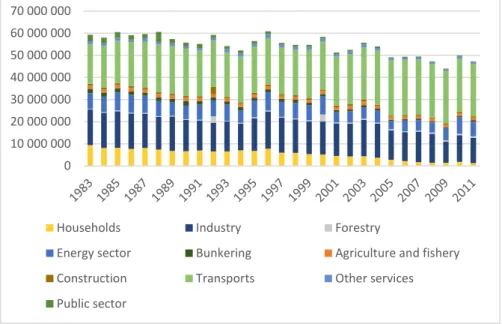
Figure 1 shows total CO2 emissions over time, based on consumption of fossil fuels for end-use in 10

Swedish sectors. Between 1983 and 2011, total emissions in Sweden have decreased from approximately 60 million tons to 48 million tons. In 1983, households accounted for roughly 16 percent of total emissions, and industries for around 27 percent. In 2011, these percentages had decreased to less than 3 percent for households and 24 percent for the industry.

Figure 1 Total CO2 emissions in Sweden 1983-2011, based on energy consumption for end use (see description in Section 0)

2.1. The general CO

2

tax and industry rebates

In 1991, the Swedish CO2 tax was implemented as a part of larger general tax reform. Until this point

in time, tax on energy had primarily been collected for fiscal reasons and as a means to reduce oil dependency after the oil crisis in the 1970s. The implementation of the carbon tax was the first time energy was taxed for environmental reasons. The tax, however, did not simply add to the previous taxes but in part replaced the existing energy tax, which was halved for fossil fuels when the new tax was introduced (Bohlin, 1998). The carbon tax was first set at a rate of 250 SEK/ton of CO2 for all fuels

except biofuel and peat, regardless of the sector in which they were being used. This was adjusted in 1992 when the tax rate was reduced for the manufacturing industry, which now paid 25 percent of the general CO2 tax rate. The rebate was sustained until 1997 when the percentage of the tax for the industry

was increased to 50 percent. Between the years 2000 and 2010, this fraction was again somewhat reduced, followed by a slight increase in 2011 (See Table 1).

0 10 000 000 20 000 000 30 000 000 40 000 000 50 000 000 60 000 000 70 000 000

Households Industry Forestry

Energy sector Bunkering Agriculture and fishery

Construction Transports Other services

(9)

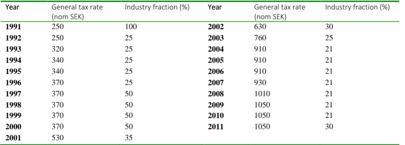
Table 1 General CO2 tax rate and the percentage of the tax paid by the industry, years 1991-2011 Year General tax rate

(nom SEK)

Industry fraction (%) Year General tax rate (nom SEK) Industry fraction (%) 1991 250 100 2002 630 30 1992 250 25 2003 760 25 1993 320 25 2004 910 21 1994 340 25 2005 910 21 1995 340 25 2006 910 21 1996 370 25 2007 930 21 1997 370 50 2008 1010 21 1998 370 50 2009 1050 21 1999 370 50 2010 1050 21 2000 370 50 2011 1050 30 2001 530 35

Source: (SEA & SEPA, 2004; Swedish Tax Agency, 2005-2011)

The level of the general CO2 tax has steadily increased from the start with a faster growth rate during

the first years of the new century. During this period a green tax reform was carried out, which meant that tax on labor was in part replaced by a higher carbon tax. Although the CO2 tax increased rapidly

during this period, it is important to mention that the industry, apart from receiving a larger rebate on the CO2 tax rate, were compensated through a lower energy tax, adjustments in the exemption rules for

the CO2 tax and a lower general wage charge (“allmän löneavgift”) (Lewin, 2009). In 2008, industries

that were a part of the EU emission trading scheme (implemented in 2005) were admitted a rebate on the carbon tax amounting to 85 percent. This amount was lowered to 70 percent in 2011 to harmonize with the average industry rebate. Apart from these general tax reductions, energy-intensive industries may be eligible for further tax cuts if the cost of the CO2 tax exceeds a certain amount of the product

sales value. (Swedish Tax Agency, 2008, 2009, 2010, 2011). An exception to the many industry reductions is the fact that fuels used as propellants are taxed equally for households and all other sectors of the economy (Swedish Energy Agency, 2006).

2.2. Other policy instruments that may influence CO

2

emissions

Although the carbon tax is the one policy instrument that has the clearest objective when it comes to reducing CO2 emissions, there is a large variety of other policy instruments that are used for the same

purpose. The policies range from economic instruments to green investment schemes. The two policy instruments which are assumed to be of particular importance in mitigating CO2 emissions are the fiscal

energy tax, which is, in fact, a set of several different taxes, and the EU emissions trading system (ETS). These two instruments are described in short below.

The energy tax

The energy tax in Sweden is levied on all non-renewable energy sources and on electricity and tall oil. More specifically, there is a separate tax on each of the following energy sources as well as on sub-categories to some of these sources: electricity, motor gasoline, oil fuels, coal fuels, liquefied petroleum gas, peat, and tall oil. Although the energy tax originally did not have an emission mitigating purpose, it has been modified over the years so that “cleaner” fuels are taxed at a lower rate than more carbon-intensive ones. This implies that the energy tax should have a similar effect to that of the CO2 tax.

The EU emission trading system

The EU emission trading system was implemented in 2005 as a way to reduce greenhouse gas emissions cost-effectively. In each year a cap is set on the total amount of CO2, N2O and PFCs (perfluorocarbons)

that may be emitted by the sectors covered by the system. Firms either receive or buy emission permits that must cover the volume of emissions they produce every year. Excess permits can either be sold or kept to cover future emissions. Firms that emit more than they have allowances for must buy the

(10)

enables emission reductions to be carried out in those plants where the cost of these measures is the lowest. In the case of CO2 emissions, the sectors that are included in the emission trading system are

power and heat generation, commercial aviation (since 2010), and energy-intensive industries (European Commission, 2017; SEPA, 2018). In other words, some of the industries included in the industrial sector in this thesis are also covered by the ETS system.

(11)

3. Previous research on the evaluation of CO

2

taxes

Given that the Swedish tax on carbon dioxide has been in place since the early 1990s, econometric ex-post studies evaluating its effect are surprisingly few. According to Skou Andersen et al. (2001, pp. 55-67), most econometric studies that had been carried out for Sweden in 2001 mainly dealt with ex-ante forecasting. The ex-post evaluations were either based on qualitative interviews or on quasi-experimental simulations of what emissions would have been, had the tax not been in place. The tendency towards simulation studies has continued since then and also seems to be the case internationally. One problem with this phenomenon is that many simulation studies assume a uniform tax rate across sectors, despite the fact that many countries – including Sweden – have exemption schemes for energy-intensive sectors (see for example literature reviews in (Lin & Li, 2011) and Morley (2012)). This implies that simulation studies are not as reliable as one would hope when evaluating carbon tax policies. A few econometric ex-post evaluations have, however, been made – mainly at aggregate, country levels (Lin & Li, 2011; Morley, 2012; Shmelev & Speck, 2018), and for industrial sectors in different countries (Bjørner & Jensen, 2002; Brännlund et al., 2014; Martin et al., 2014). The results at the aggregate level are somewhat ambiguous, with some studies finding no significant effect of the carbon tax on emissions. On the other hand, the results for industries show that CO2 taxes have

significant negative effects on emissions. Fewer studies have been made on households, but one Swedish study implies that environmental taxes reduces demand for energy in households, and even more so than changes in fuel prices (Ghalwash, 2007).

Lin and Li (2011) estimate the effect of the CO2 tax on total emissions for five countries, among which

Sweden is one. The authors use a difference-in-difference approach to evaluate whether countries that have adopted a CO2 tax have a significantly slower growth rate of emissions than countries without such

a tax. They apply this method for Sweden, Denmark, Norway, Finland and the Netherlands, using a panel of 13 EU and OECD member countries as a control group for the time period 1981-2011. None of the control countries had implemented a carbon tax during this period. The authors also control for GDP per capita, industry structure, energy price and gross domestic R&D expenditure. The estimated model shows that all countries but Norway had point estimates that indicated slower growth rates in emissions than the control group. However, the only country with a significant estimate was Finland. The reason, according to the authors, is that Finland, unlike the other countries in the study, makes few tax reductions for the industry. Sweden, on the other hand, gives significant tax reductions to large parts of the industry.

A recent paper by Shmelev & Speck (2018) also estimates the effect of the carbon tax on total emissions in Sweden. Their time-series analyses show no significant effect of the general carbon tax on CO2

emissions, but a negative and significant effect of the specific carbon tax on petrol and the combined energy and carbon taxes on coal and liquefied petroleum gas. The authors conclude that the decline in CO2 emissions in Sweden is not primarily due to the carbon tax. Instead, the oil price, as well as

technological development, are seen as the main contributors.

Morley (2012) examines the effect of environmental taxes on greenhouse gas emissions in the European Union and Norway. The author constructs two measures of the level of environmental taxation in each country: the revenue from environmental taxes as a share of GDP and the revenue of environmental taxes as a share of the total tax revenue. Using a panel of 25 countries for the years 1995-2006, the author then tests if a higher level of environmental taxation is associated with lower levels of emissions. The results show that environmental taxes, as a share of either GDP or total tax revenues, have a significant negative impact on greenhouse gas emissions, but not on energy consumption. Due to the significant effect on emissions, the author suggests that the exemptions faced by large parts of the industry have had only little effect on pollution levels. This is in contradiction to the findings in Lin and Li (2011), above.

(12)

Brännlund et al. (2014) study the effect of the carbon tax on environmental efficiency performance in the Swedish manufacturing industry (the same sector demarcation as in this thesis). By using firm-level data on actual tax payments and CO2 emissions, effective carbon taxes for each respective firm are

calculated as total tax payments divided by total CO2 emissions. Environmental efficiency performance

is defined as the change in the output to CO2 ratio between t and t+1, while the CO2 tax and other

covariates are defined for period t. This way potential endogeneity issues are avoided. Fixed-effects and random-effects models are estimated for the manufacturing industry as a whole, for different sub-sectors, and for energy intensive and non-energy intensive sectors respectively. The models control for other influencing factors such as the price of fossil fuels, cost share of fossil fuels, capital intensity, firm size, and a time-trend. Results show that the tax had significantly increased environmental performance, i.e. reduced carbon-intensity, in the manufacturing industry. Furthermore, since emissions have declined in the sector during the period, the authors conclude that there has been an absolute decoupling of emissions from output. It was also shown that firms are more sensitive to changes in the carbon tax than they are to changes in fuel prices. This means that apart from just raising the price, a tax might signal that the rise is more permanent than other price fluctuations and induce firms to invest more in energy conservation. A clear strength of the paper is the fact that they have access to firm-specific, actual tax payments. This means that they can account for all firm-specific exemptions from the general CO2 tax

rate, something that couldn’t be done in this thesis. It is worth noting that, although the carbon tax has had a significant effect on environmental performance, we cannot say if this has acted solely through emission abatement, or if the tax may actually have had a positive effect on production. This is somewhat counterintuitive, but the authors themselves mention that this might be the case if the tax forces firms to use energy inputs more effectively.

Bjørner & Jensen (2002) evaluate the CO2 tax in the Danish industry. Their objective is to analyze

energy demand in the Danish industry to determine how it has been influenced by the carbon tax as well as by two other policies: voluntary agreements and subsidies. The authors estimate a double-logarithmic function where total energy use is a function of value added, energy price (including the tax) and the existence of an agreement and/or subsidy. The effect of the tax is in other words indirectly approximated by the price-elasticity of energy demand. Using estimates for different sub-sectors, Bjørner and Jensen (2002) find a weighted mean of the energy demand-elasticity of -0.44. In other words, a 10 percent increase in the total energy price induces a decrease in energy consumption in the Danish industry by 4.4 percent. This is an interesting finding and serves as a valuable comparison to the results in this thesis. However, the study differs in two important respects from the present paper. First, the variable of interest is energy consumption rather than CO2 emissions. This means that unless all emission abatement is due

to energy conservation, the elasticities are not fully comparable. Second, the study by Bjørner and Jensen (2002) evaluates the tax merely indirectly through the total price-elasticity, where the price includes both fuel prices and the carbon tax, and thus disregard a potential signaling effect.

An evaluation by Martin et al., (2014) of the Climate Change Levy, CCL, (a kind of CO2 tax) in the UK,

also indicates a significant effect of carbon taxes when it comes to reducing emissions in the industry sector. By using eligibility for the CCL as an instrument in a difference-in-difference model, the authors estimate the effect of paying the full CCL (corresponding to about 15 percent of a firm’s energy expenditure), compared to paying a reduced tax (about 3 percent of energy expenditures). The findings show that the CCL had reduced electricity consumption by 22.6 percent, although no significant reductions were seen for gas or solid fuels. When estimating the effect on CO2 emissions, the point

estimate was -8.4 percent but not significant, something the authors attribute to the small sample size and “the noisy estimates of the tax response for fuels other than electricity”. Nevertheless, because of the large and significant reduction in electricity consumption, it is concluded that there actually has been a real reduction in CO2 emissions in the industrial sector, as a result of the Climate Change Levy.

Regarding the household sector, one study estimates the effect of the Swedish CO2 tax, not on emission

(13)

react differently to increases in environmental taxes than to price changes. By using a three-stage budgeting model and time-series data on consumption of non-durable goods, the author estimates own-price elasticities for food, residential heating, transport and other goods, as well as the own-price elasticities of the environmental taxes associated with heating and transport. For residential heating in general, the price-elasticity is -0.07 for the energy price and -0.36 for the energy tax. The difference between the elasticity estimates is statistically significant, implying that there is a signaling effect of the energy tax on the demand for heating. This relationship also holds for different inputs in heating. The price-elasticities for the taxes on electricity used for heating, district heating and heating oil are -1.80, -1.83 and -1.58 respectively. In other words, energy taxes on these goods lead to a relatively large reduction in demand, implying that energy taxes could also be effective in reducing emissions from these sources. This is an interesting result as the main source of emissions in the household sector, as defined in this thesis, is residential heating. It is important to mention, however, that Ghalwash (2007) makes no distinction between different types of energy taxes (fiscal energy taxes versus the carbon tax), but analyzes the effect of total taxes on the demand for different energy commodities. In this way, the paper differs from the present thesis. Nevertheless, it gives important insights to how households react to tax changes, as opposed to other price changes.

(14)

4. Theoretical framework

The effect of a carbon tax is estimated as the impact on demand for fossil fuels by industry and households separately. A carbon tax corrects for the negative externality from CO2 associated with the

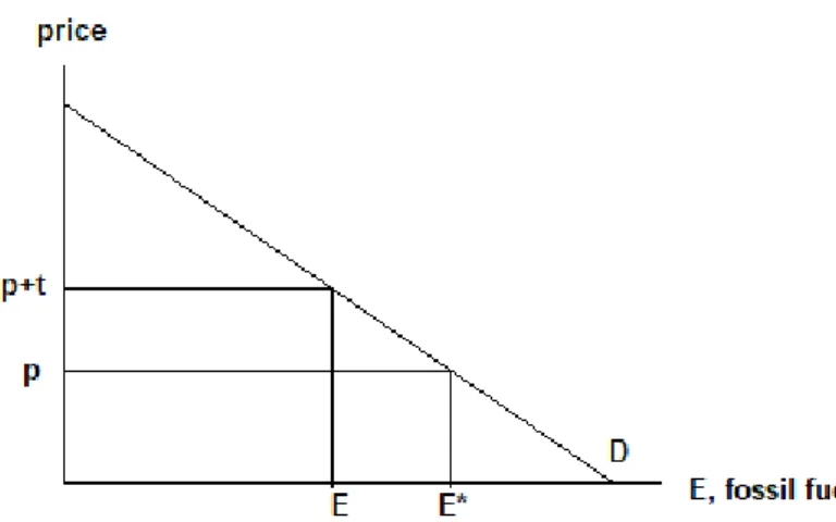
use of fossil fuels. In the simplest example, one can assume a firm or household demanding fossil fuel, E, in Figure 2.

Figure 2 Demand for fossil fuel with and without tax

The demand curve D reflects the value of the marginal product of fossil fuel for the industry, and the marginal utility of consumption of fossil fuel for households. Without a carbon tax, t, in Figure 2, the demand for fossil fuel at the price p is E*. The introduction of the tax reduces demand, and hence CO2

emissions, to E.

The demand for fossil fuel by the industry is derived from the maximization of profits. Imagine a representative firm that produces Q units of output using labor, L, capital, K and energy, E and assume that the effective price of energy is the sum of the market price of energy and the unit carbon tax. Then the profit function can be expressed as,

Π = 𝑃𝑄 − 𝑤𝑙𝐿 − 𝑤𝑟𝐾 − (𝑤𝑒+ 𝑡𝑐)𝐸,

where P is output price, w l_{is wage, w}r_{is the interest rate, w}e_{is the market price of energy and t}c_{is the}

carbon tax. Furthermore, assume that the energy used by the firm corresponds to a constant amount of CO2 emissions and for simplicity, assume that this amount is one unit. Then the profit function can be

rewritten as,

Π = 𝑃𝑌 − 𝑤𝐿 − 𝑟𝐾 − (𝑤𝑒+ 𝑡𝑐)𝐶𝑂₂,

which is non-decreasing in P and non-increasing, homogeneous of degree 1, convex and continuous in

w l_{, w}r_{, w}e_{and t}c_,

Taking the first order conditions and solving for K, L and CO2 as functions of P, w l, w r, w e+t c gives

us the demand functions for each of the inputs. These are inserted back into the profit function to get the optimal level of production Π∗_{(𝑃, 𝑤}𝑙_{, 𝑤}𝑟_{, 𝑤}𝑒_{and 𝑡}𝑐_).

Applying Hotelling’s lemma we get the optimal demand for fossil fuel and CO2 emitted by the firm as:

− 𝜕Π

∗

𝜕(𝑒 + 𝑡)= 𝐶𝑂2(𝑃, 𝑤

𝑙_{, 𝑤}𝑟_{, (𝑤}𝑒_{+ 𝑡}𝑐_{)) = 𝐶𝑂} 2∗

This is of course a simplification, as in reality, firms may choose between several energy inputs associated with different prices and carbon tax rates.

(15)

For a representative household, assume instead that utility is a function of a vector of consumer goods,

Q, and energy, E, and that the household maximizes its utility subject to the budget constraint. As before,

we make the simplification that one unit of energy corresponds to one unit of CO2 emissions. Then the

maximization problem can be written as, max

𝑄,𝐸 𝑈(𝑄, 𝐸) 𝑠. 𝑡. 𝑀 = 𝑃𝑄 + (𝑤

𝑒_{+ 𝑡}𝑐_{) 𝐶𝑂} 2,

which translates into the Lagrangian

ℒ = 𝑈(𝑄, 𝐸) + 𝜆(𝑀 − 𝑃𝑄 − (𝑤𝑒+ 𝑡𝑐) 𝐶𝑂2)

M is the exogenous income, P is the price for a vector of consumer goods, e w is the market price of energy and t c is the carbon tax associated with one unit of CO2. Taking the first order conditions of the

Lagrangian and solving for Q* and CO2* gives us the optimal levels of Q and CO2 as functions of M, P

and (we+tc). Inserting these parameters into the original utility function gives us the indirect utility

function that only depends on prices and income,

𝑉(𝑃, (𝑤𝑒+ 𝑡𝑐), 𝑀) By Roy’s identity, we have that

𝐶𝑂2∗= 𝐶𝑂2(𝑃, 𝑀, 𝑤𝑒, 𝑡𝑐) = −

𝜕𝑉 𝜕(𝑤𝑒_{+ 𝑡}𝑐₎

𝜕𝑉 𝜕𝑀

In summary, the amount of CO2 that is emitted by firms depends on the output price, wage rate, interest

rate, energy prices and the carbon tax. Emission by household is a function of income, output and energy price, and the carbon tax.

Of course, in reality, the situation is much more complex. Firms can substitute between different types of energy, between energy and labor, and can invest in new technology in order to use energy more efficiently. This means that production does not necessarily need to decrease until the optimal level with original production methods, is met. Instead, it is more likely that the tax decreases production to some extent, while at the same time lowering marginal external costs through technological development.

(16)

5. Data

Following the theoretical framework, the data used in this thesis are:

For households: CO2 emissions, real GDP per capita, consumer price index (excl. energy), total real

energy prices and real CO2 taxes.

For industries: CO2 emissions, real industry wages, real interest rate or stock market dividends (two

different proxies for the price of capital), producer price index, total real energy prices, and real CO2

taxes.

The sources of these data are described in the sections below. In some cases, the required data has not been readily available and has instead been computed using different data sources. These computations are also outlined below and, in further detail, in the appendices. The data set covers the period 1983-2011, since this is the longest available time series on energy consumption.

5.1. CO

2

emissions

Total CO2 emissions in both sectors are calculated by multiplying energy demand for various energy

sources, by the emission factors associated with each respective energy source. Data on energy demand are collected from the annual energy balances produced by the Swedish Energy Agency and available through Statistics Sweden (Statistics Sweden, 2011, 2013). The sectors studied in this thesis are based on the sector definitions in the energy balances, where households correspond to item 7.8 Use in

households (lodgments and other), and industries (more specifically, the manufacturing industry)

correspond to item 7.3 Use in industry (SNI 10-37)4_{. SNI is a Swedish sector classification system and}

10-37 refers to the specific sub-sectors that make up the manufacturing industry (Statistics Sweden, 2014).

Since the focus of the present thesis will be on the use of energy in Swedish households and industries, the data is collected from the item “energy for end-use” (“slutlig energianvändning”). At the time of the collection of the data, there were two different datasets in the Energy balances: one for the years 1983-2009 and one for the years 2007-2011. These are based on two different versions of the sector classification system mentioned above (SNI 2002 and SNI 2007 respectively). The two data sets have been chained to avoid any jumps due to differences between the two sets.5

There are in total 16 energy source in the energy balances6_{. Of these, 14 are fuels such as coal, gasoline}

and natural gas7_{. The remaining two are electricity and district heating. Emission factors can be obtained}

from the Swedish Environmental Protection Agency (SEPA, 2015) for each of the 14 fuels between 1990 and 2014. The emission factors for 1983-1989 are assumed to be the same as for 1990, which is plausible since emission factors differ only marginally over the years. The emission factors in terms of tons of CO2 per TJ are multiplied by the energy consumption for each respective fuel in TJ to obtain

total emissions of CO2 for each sector in each year. One exception is tall oil. Since the emission factors

from SEPA are based on the direct emissions from combustion and do not take into account life-cycle effects, the emission factor for tall oil is positive and high, even though tall oil is a renewable energy source. For this reason, tall oil is instead assumed to have zero net emissions.

For electricity and district heating there are no available emission factors for the time period at hand. Instead, emissions will be approximated by calculating the emissions associated with fuel inputs in the production of electricity and district heating, respectively. Data on fuel inputs and energy production for

4_{In Swedish: 7.8 Användning inom hushåll (bostäder och annat) and 7.3 Användning inom industry (SNI10-37).} 5_{This is done by simply relating energy demand in the two data sets for year 2009, and assuming that this}

relation also holds for the years 2010-2011.

6_{Not counting crude oil, which is presented in the energy balances although virtually zero.}

7_{The rest are: coke, tall oil/oil pitch, petroleum coke, liquefied petroleum gas, light distillates, diesel oil,}

(17)

electricity and district heating are collected from the Swedish Energy Agency and their annual publication “Energiläget i siffror”(SEA, 2018). The approach used to compute emissions from each energy type is outlined below.

Emission factors for electricity and district heating

In table 6.3 in Energiläget i siffror 2018 (SEA, 2018) fuel inputs in electricity production are divided into five different sources: biofuels, coal (including coke-oven and blast furnace gas), petroleum products, natural gas and “other fuels”. For simplicity, biofuels are assumed to have zero net emissions. Emission factors for coal will be used for the second fuel group even though it also includes some coke and furnace gas. Emissions from petroleum products are approximated using emission factors for heating oils 2-5, which are the more commonly used oils in energy plants (SPBI, 2010). The last category, “Other fuels”, consists of fossil waste and peat (Swedish Energy Agency, 2015, p. 49). The emission factors for these in heat and power plants are 94.3 and 107.3 tons per TJ for all years, according to the Swedish Environmental Protection Agency (SEPA, 2015). The mean value, 100.8, will be used to approximate emissions from “other fuels”. As before, year specific emission factors will be used for the years 1990-2011. Emission factors for the years 1983-1989 will be approximated by using the emission factors for 1990.

The Swedish Energy Agency expresses fuel consumption in terms of TWh. This will be converted into TJ using a factor of 3600 and multiplied with the above emission factors for each year to obtain total CO2 emissions from domestic electricity production. Total CO2 will then be divided by total electricity

production from table 6.2 in (SEA, 2018) to get an electricity emission factor in tons of CO2/TJ. The

computed values for electricity emission n factors range from about 3 to 7 tons of CO2/TJ for most years

(although there are a few years that stand out with higher values up to 12.8 CO2/TJ in the most extreme

case). This is most likely an understatement of the true amount of emissions associated with electricity consumption. For instance, Martinsson et al. (2012) found values to be between approximately 28 and 39 CO2e/TJ in 2009, compared to 4.4 CO2e/TJ for the same year in the present thesis. The report by

Martinsson et al. (2012) takes into account electricity trading with other countries, as well as other greenhouse gases, apart from just carbon dioxide, which may to some extent explain the differing results. An implicit assumption in the computation of emission factors for electricity is that all production of electricity is used for domestic consumption and that there is no import. This is not completely true, although the net import of electricity is small or even negative for most years. Another potential problem is that the data does not include electricity production from wind, hydro and nuclear power, each of which has been found to produce positive emissions in life cycle analyses (Miljöfaktaboken 2011, p. 95-101).

The approach for computing emission factors for district heating is similar to that for electricity. One difference, however, is that there are another three energy sources used as inputs in the production of district heating, apart from the five listed above. These are electric boilers, heat pumps and waste heat (“elpannor”, “värmepumpar” and “spillvärme” in table 7.2 in (SEA, 2018)). Electric boilers heat water for the heating network using electricity, heat pumps recycle heat from sewage and “waste heat” refers to the recycling of residual heat from industries (Statistics Sweden, 2016). For simplicity, emissions associated with heat pumps and waste heat will be assumed to be zero, since these are simply ways of recycling energy. For electric boilers, we will use the emission factors of electricity calculated above. As before the use of fuel inputs will be converted from TWh to TJ and then multiplied by their respective emission factors for each year. Annual emissions from the production of district heating will then be divided by the total production of district heating, also in table 7.2 in Energiläget i siffror 2018 (SEA, 2018). The computed emission factors for electricity and district heating can be found in Appendix A.

(18)

5.2. The CO

2

tax

General carbon tax rates in SEK/ton of carbon, are collected from two sources, the 1998-2011 Tax Statistical Yearbooks (Swedish Tax Agency) and from a report produced by the Swedish Energy Agency and the Swedish Environmental Protection Agency (SEA & SEPA, 2004). The sources give information on both general tax rates and tax rates for industries, but not on firm-specific reductions.

5.3. Total energy prices

The total energy price is approximated by the sum of the energy price, the carbon tax and the two most important energy taxes. The carbon tax in each sector and year is found in Table 1 in section 2. The energy price and energy taxes are described below.

Energy prices

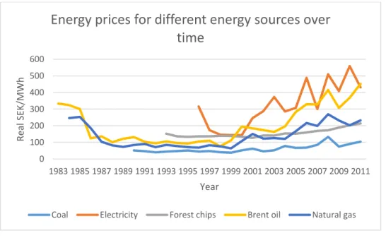
Energy prices are approximated by using Brent oil prices (SEA, 2018) and have been converted from nominal US dollars to real SEK using consumer price index (Statistics Sweden, 2015c) and exchange rates (Riksbanken, 2015). Brent oil is a type of crude oil which is often used as a reference when determining oil prices (VA Finans, 2018). Figure 3 shows energy prices over time for coal, electricity, forest chips (a type of biofuel), Brent oil and natural gas. As you can see, Brent oil price is a good – albeit not perfect – approximation of prices for most other energy sources. The main exceptions are the electricity price in the year 1996 (there are no earlier data) and coal prices for the more recent years, which have increased at a slower rate than oil prices.

Figure 3 Energy prices over time for coal, electricity, forest chips, Brent oil, and natural gas

Source: (SEA, 2018)

Energy taxes

The energy tax is in fact not one but several different taxes set on different sources of energy. The analysis in this thesis will include the energy taxes for electric energy and heating oils (domestic heating oil and heavy fuel oil), which are deemed to be the most important energy taxes faced by households and industries (see Appendix B). The tax rates are collected from the Swedish Tax Agency (Swedish Tax Agency, 2018).

The energy taxes are further differentiated according to for instance environmental standard or the type of user, and these sub-categories vary over time. In order to get continuous energy tax variables, some choices have been made regarding which categories are used for which years. These decisions can also be found in Appendix B. Furthermore, the energy taxes are expressed in different units depending on

0 100 200 300 400 500 600 1983 1985 1987 1989 1991 1993 1995 1997 1999 2001 2003 2005 2007 2009 2011 Re al SE K/MWh Year

Energy prices for different energy sources over

time

(19)

the energy type. The electricity tax, for instance, is expressed in öre8_{/kWh, whilst the tax on oil is stated}

in SEK/m3_{. All taxes will be converted into real SEK/TJ.}

5.4. Other data sources

GDP per capita is calculated by dividing total GDP by the number of Swedish inhabitants. Both GDP and population records are collected from Statistics Sweden (Statistics Sweden, 2015a; b).

Data on nominal wage rate per hour in the manufacturing industry is obtained from Historia.se (2018). Two measures of the cost of capital are used: interest rate on long term governmental bonds, and stock market dividend yields. Both are found at Historia.se (2018b). These are corrected with the inflation rate to obtain real values.

Producer price index shows the development of outputs produced in Sweden and is obtained from Statistics Sweden (2018).

Consumer prices of other goods and energy are calculated by correcting the consumer price index (CPI) with the increase in energy prices. This is made by multiplying the energy price with the share of energy consumption of total consumption obtained from Swedish Energy Agency (SEA, 2017) and estimate the associated annual rate of change which is deducted from the CPI. Data on shares of total consumption is not available for each year since 1983, and shares for missing years have been approximated by average annual changes between the years with data.

5.5. Descriptive statistics

In the tables below you will find summary statistics for all variables in the two sectors. Table 2 Summary statistics for the household sector

Variable T Mean Std. Dev. Min Max

CO2 emissions 29 8339468 2999463 3578702 1.30e+07 CO2 tax rate 29 504.7846 404.6077 0 1093.614 GDP per capita 29 298060.6 55260.02 221383 385598.8 Household Energy Price 29 29 161978.3 78595.38 78810.19 CPI (excl. energy) 29 77.33962 16.79117 42.577 99.55328

(20)

Table 3 Summary statistics for the industry

Variable Obs Mean Std. Dev. Min Max

CO2 emissions 29 1.48e+07 1816157 9738535 1.73e+07

CO2 tax rate 29 145.615 107.2107 0 342.7128 Real Wage 29 147.8922 22.84543 114.6973 185.7514 Industry Energy price 29 84070.15 33449.01 36173.75 161688.2 PPI 29 117.1141 7.191148 106.0497 131.8443

Real interest rate 29 3.927674 2.405929 -1.046645 8.710724

Stock market div. 29 2.736207 1.220031 1.45 7.26

Figure 4 and Figure 5 show how the statutory carbon tax rates have developed over time for the household and industry sectors respectively. As shown in the graphs, the industries have faced a significantly lower tax rate than household consumers. Furthermore, the tax rate has increased at a much slower pace. It is important to note that the general tax rate for the industry in many cases is higher than the actual tax paid by individual firms. This is due to the fact that industries may apply for further, firm-specific rebates that are not captured by this data. According to Brännlund et al. (2014), the median effective tax rates for manufacturing firms ranged from around 130 nominal SEK/ton in 1991 to just over 150 SEK per ton in 2004. Moreover, from 2008, firms that are a part of the EU emissions trading system have a general rebate of 70-85 percent of the CO2 tax. (Lewin, 2009) The tax rate for the industry

is thus an overstatement for most, if not all, years of the sample - and to an even larger extent from 2008. Figure 4 Carbon tax rate for households

Source: (SEA & SEPA, 2004; Swedish Tax Agency, 2005-2011) 0 200 400 600 800 1000 1200 1991 1993 1995 1997 1999 2001 2003 2005 2007 2009 2011 Re al SE K/to n CO2 Year

(21)

Figure 5 General carbon tax rate for industries

Source: (SEA & SEPA, 2004; Swedish Tax Agency, 2005-2011)

In Figure 6 and Figure 7, emissions from the two sectors are shown. Emissions have been decreasing in both sectors since the beginning of the sample, with a few exceptions. Notably, there was no significant shift downwards in either sector after 1991 when the carbon tax was introduced. As a matter of fact, emissions increased slightly in the household sector between 1991 and 1997. Industries continued an already downward sloping trend in CO2 emissions until 1995 when emissions shifted sharply upwards.

Regarding the entire time period, both sectors have decreased their emissions between 1983 and 2011. Figure 6 CO2 emissions from households 1983-2011

Figure 7 CO2 emissions from the industry 1983-2011 0 50 100 150 200 250 300 350 400 1991 1993 1995 1997 1999 2001 2003 2005 2007 2009 2011 Re al SE K/to n CO2 Year 0 2000000 4000000 6000000 8000000 10000000 12000000 14000000 1983 1985 1987 1989 1991 1993 1995 1997 1999 2001 2003 2005 2007 2009 2011 0 2000000 4000000 6000000 8000000 10000000 12000000 14000000 16000000 18000000 20000000 1983 1985 1987 1989 1991 1993 1995 1997 1999 2001 2003 2005 2007 2009 2011

(22)

6. Econometric methodology

A stepwise regression analysis will be performed in each of the sectors. The models are expressed in a log-linear form so that the elasticity of emissions with respect to the CO2 tax can be derived. The

formulation of the final models in each of the sectors is outlined below. Household sector:

𝑙𝑛𝐶𝑂_2𝑡= 𝛽0+ 𝛽1𝑙𝑛𝐺𝐷𝑃𝐶𝑎𝑝𝑡 + 𝛽2𝑙𝑛𝑜𝑝𝑖𝑡+ 𝛽3𝑙𝑛ℎ𝑝𝑖𝑡+ 𝛽4𝑙𝑛𝐶𝑂2𝑇𝑎𝑥𝑡+ 𝛽5𝑙𝑖𝑛𝑒𝑎𝑟 + 𝜀𝑡

The variables in the household regressions are GDP per capita, a consumer price index excluding energy prices (opi), total energy prices for households (hpi), the household CO2 tax and a linear time trend. 𝜀_𝑡

is the error term. Industrial sector:

𝑙𝑛𝐶𝑂_2𝑡 = 𝛽0+ 𝛽1𝑙𝑛𝑟𝑤𝑡 + 𝛽2𝑙𝑛𝑟𝑖𝑡(𝑙𝑛𝑟𝑖_𝑎𝑙𝑡) + 𝛽3𝑙𝑛𝑝𝑝𝑖𝑡+ 𝛽4𝑙𝑛𝑖𝑝𝑖 + 𝛽5𝑙𝑛𝐶𝑂2𝑇𝑎𝑥𝑡+ 𝛽6𝑙𝑖𝑛𝑒𝑎𝑟

+ 𝛽7𝐸𝑇𝑆 + 𝜀𝑡

The variables in the industrial sector are real wage (rw), the real interest rate (ri) or stock market dividend (ri_alt), producer price index (ppi), total energy prices for industries (ipi), the CO2 tax, a linear time

trend and a dummy for the years when the ETS sector was in place.

The linear time trend is included to capture any general tendencies towards for instance increased environmental awareness and energy conservation. In the following sections, unit root tests of the variables are performed to determine the correct regression model to be used in the analysis.

6.1. Unit root tests

An important assumption when analyzing any time series data, is that the time series is stationary. Simply put, this means that the mean and variance are constant over time and that the covariance only depends on the distance between the two time periods and not on the actual value of t at which the covariance is computed. (Gujarati, 2011, p. 216). Since the dataset in this thesis extends over almost thirty years, the risk of non-stationarity is large and it is therefore important to test for stationarity. This is done through unit root testing. Three different unit root tests are performed on the dependent variable CO2: an augmented Dickey-Fuller (ADF) test without lags or time trend, an ADF test with a time trend

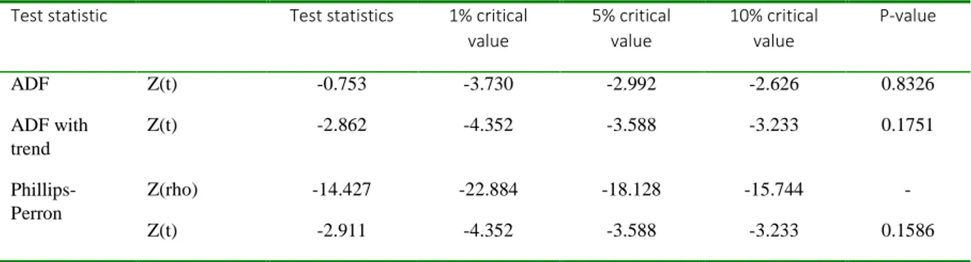
and a Phillips-Perron test with a time trend. The Phillips-Perron test is similar to the ADF test but with test statistics that have been made robust to serial correlation (STATA, 2018). The null hypothesis, in either case, is that the variable is a random walk, and the alternative hypothesis is that the variable is stationary. As is shown in the table below, all three tests fail to reject the null hypothesis.

Table 4 Unit-root tests of the CO2 variable

Test statistic Test statistics 1% critical value 5% critical value 10% critical value P-value ADF Z(t) -0.753 -3.730 -2.992 -2.626 0.8326 ADF with trend Z(t) -2.862 -4.352 -3.588 -3.233 0.1751 Phillips-Perron Z(rho) -14.427 -22.884 -18.128 -15.744 - Z(t) -2.911 -4.352 -3.588 -3.233 0.1586

The fact that the dependent variable, is non-stationary, indicates that there might be a problem of cointegration in the data set. This in turn could lead to problems of spurious regression. To control for this, the Fully Modified Ordinary Least Squares will be used in the analysis.

(23)

7. Results

7.1. Households

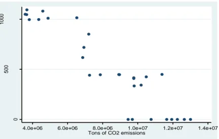
In the graphs below carbon emissions in households are plotted against the total energy price and carbon tax, respectively. It appears that there is an overall negative relationship between the two variables – in other words, a higher price of energy or CO2 tax is associated with lower CO2 emissions

from households.

Figure 8 Total energy price and CO2 emissions, households

Figure 9 Carbon tax and CO2 emissions, households

Before doing any estimations, it is necessary to check for multicollinearity among the explanatory variables. This is done by doing pairwise correlations among the regressors. A high correlation coefficient indicates that variables are collinear and, generally, these two variables should not be included in the same regression. Nevertheless, regarding some of the variables, these will be included in the same models (even though there might arise collinearity problems) if there is a theoretical motivation for doing so. Any conclusions about the regression estimates should, however, be made with caution.

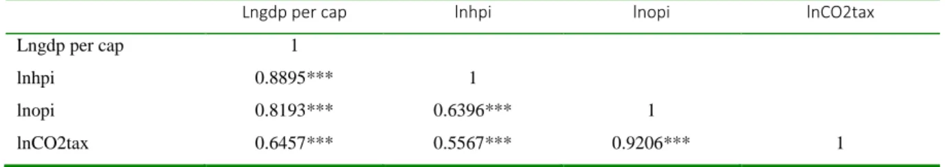
Table 5 shows pairwise correlations among the explanatory variables GDP per capita, household energy prices (hpi), consumer price index of non-energy consumption (opi) and the CO2 tax. It is noticeable

1 0 0 0 0 0 1 5 0 0 0 0 2 0 0 0 0 0 2 5 0 0 0 0 3 0 0 0 0 0 H H b re n t p ri ce + ta xe s

4.0e+06 6.0e+06 8.0e+06 1.0e+07 1.2e+07 1.4e+07 Tons of CO2 emissions

0 5 0 0 1 0 0 0 R e a l SEK/ to n

4.0e+06 6.0e+06 8.0e+06 1.0e+07 1.2e+07 1.4e+07 Tons of CO2 emissions

(24)

the carbon tax is highly correlated with the consumer price index (r>0.9). This indicates that there may be a problem of multicollinearity among the regressors in the following analysis.

Table 5 Pairwise correlations for explanatory variables in household data. * Indicates significance at 5% level.

Lngdp per cap lnhpi lnopi lnCO2tax

Lngdp per cap 1

lnhpi 0.8895*** 1

lnopi 0.8193*** 0.6396*** 1

lnCO2tax 0.6457*** 0.5567*** 0.9206*** 1

Table 6 shows the results of a stepwise FMOLS regression. In the baseline model, CO2 emissions are

regressed on GDP per capita and prices of non-energy goods, “opi”. In model 2, total energy prices (hpi) are added to the model, and in model 3, the carbon tax is included. Because of the high correlation between consumer prices and the CO2 tax, the variable opi is omitted from the final regression but lowers

the goodness of fit (increases Long Run SE).

The energy price elasticity, which includes all environmental taxes is negative (-0.2442) in model 3. The coefficient for the carbon tax is, however, positive and significant, with a point estimate of 0.016, implying that the carbon tax signals to households to emit more than they would have at a regular price rise. This an unexpected result and contradicts the findings in Ghalwash (2007) on the effect of environmental taxes on demand for energy goods used for domestic heating (which is essentially what is measured here). Ghalwash (2007) finds a price elasticity of -0.07 and a tax elasticity of -0.36, i.e. a stronger, negative effect of the tax on energy demand. The coefficients for GDP per capita and the time trend are significant and negative, which explains why the carbon tax and CO2 emissions are negatively

related in the graphical analysis but not in the regression estimations. The estimate for consumer prices is negative in model 3, but not significant. In the first two models, however, the estimates for opi are positive and significant, as one would expect if there is a substitution between fossil fuels and other goods.

Table 6 Results from FMOLS regression on household emissions

(1) (2) (3) (4)

VARIABLES lnCO2 lnCO2 lnCO2 lnCO2

lnGDPCap -0.9645*** -1.0426*** -0.6482** -0.6193** (0.2339) (0.2250) (0.2815) (0.2861) lnopi 0.6374*** 0.4136** -0.3629 (0.1433) (0.2007) (0.3410) lnhpi -0.0944 -0.2442*** -0.1623*** (0.0643) (0.0866) (0.0520) lnCO2tax 0.0160*** 0.0122*** (0.0050) (0.0035) linear -0.0427*** -0.0306*** -0.0220* -0.0338*** (0.0079) (0.0110) (0.0131) (0.0080) Constant 25.8909*** 28.7818*** 28.7970*** 26.0744*** (3.2981) (3.6368) (4.2108) (3.4272) Observations 28 28 28 28 R-squared 0.9378 0.9350 0.9310 0.9406 Adjusted R-squared 0.930 0.924 0.915 0.930 Long Run SE 0.0447 0.0420 0.0485 0.0497 Bandwidth(neweywest) 32.79 39.64 17.32 17.69

Standard errors in parentheses *** p<0.01, ** p<0.05, * p<0.1

(25)

7.2. Industry

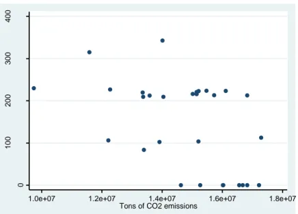
In the figures below, CO2 emissions in the industry are plotted against the total energy prices and the

carbon tax. Just as in the household sector, emissions seem to be negatively related to both the energy price and the tax, although the relationship is less clear in the industry.

Figure 10 Total energy price and CO2 emissions, industry

Figure 11 Carbon tax and CO2 emissions, industry

Table 7 shows the correlation matrix for the explanatory variables in the industry sector. The one correlation which is relatively high (r=0.8859) is that between the CO2 tax and the producer price index,

ppi. 0 5 0 0 0 0 1 0 0 0 0 0 1 5 0 0 0 0 in d u st ry b re n t p ri ce + ta xe s

1.0e+07 1.2e+07 1.4e+07 1.6e+07 1.8e+07

Tons of CO2 emissions

0 1 0 0 2 0 0 3 0 0 4 0 0 R e a l SEK/ to n

1.0e+07 1.2e+07 1.4e+07 1.6e+07 1.8e+07

(26)

Table 7 Pairwise correlations for explanatory variables in household data. * Indicates significance at 5% level.

Lnrw lnri Lnri_alt lnipi lnppi lnCO2tax

lnrw 1 lnri -0.3246* 1 Lnri_alt 0.5293*** -0.5030*** 1 lnipi 0.3464* -0.4089** 0.5511*** 1 lnppi -0.5790*** 0.2241 -0.1120 0.3727** 1 lnCO2tax 0.6862*** -0.2732 0.2660 -0.2142 -0.8859*** 1

Table 8 shows the stepwise FMOLS regressions for the industry sector with two alternative measures of the price of capital. In models 1-4, the real interest rate (ri) is used and in models 4-8, the stock market dividend (alt_ri) is included instead. The regression is done in four steps. The first model includes real wage, price of capital, and producer price index. Next, price of energy is added, followed by the addition of the carbon tax. In the fourth model in each sub-set, the producer price index is excluded due to its high correlation with the carbon tax. Finally, in model 9, a dummy for the years with the emission trading system, ETS, is added to the model with the best fit.

Regarding the long run standard errors, the preferred model is model 7. This model includes all explanatory variables, with the stock market dividend as the measure of the price of capital. The estimate for the energy price is negative, as expected, although not significant. This can be compared to Bjørner and Jensen (2002) who found a significant price elasticity in the Danish industry of -0.44. The coefficient for the carbon tax is, on the other hand, significant and negative, with a point estimate of -0.008. This is in line with the findings in Brännlund et al. (2014), who found that the Swedish manufacturing industry responds more strongly to the carbon tax than to rises in fuel prices. The other coefficients of the model also have the expected signs. The positive coefficients for the price of labor and capital indicates that there is a substitution between these input factors and fossil fuels. The negative estimate for the producer price index suggests that an increase in prices reduces production and hence emissions. The linear time trend, which captures for instance attitude changes and technological development, shows that there has been an overall tendency to reduce emissions over time. When the ETS-dummy is added to the model, coefficient for ETS is negative and significant, but this does not change the estimate for the CO2 tax,

(27)

Table 8 Results from FMOLS regression on industry emissions

(1) (2) (3) (4) (5) (6) (7) (8) (9)

VARIABLES lnCO2 lnCO2 lnCO2 lnCO2 lnCO2 lnCO2 lnCO2 lnCO2 lnCO2

lnrw 2.135*** 1.636*** 0.924*** 1.438*** 1.844*** 1.879*** 1.414*** 1.895*** 1.093*** (0.568) (0.231) (0.308) (0.475) (0.176) (0.150) (0.132) (0.237) (0.172) lnri 0.014 0.022* 0.021 -0.017 (0.026) (0.012) (0.013) (0.019) lnppi -1.929*** -1.812*** -2.296*** -1.547*** -1.474*** -1.898*** -1.242*** (0.428) (0.189) (0.239) (0.125) (0.128) (0.115) (0.171) lnipi 0.032 0.042 -0.130*** -0.014 -0.014 -0.123*** 0.009 (0.027) (0.031) (0.039) (0.017) (0.013) (0.020) (0.017) lnCO2tax2 -0.011*** 0.001 -0.008*** 0.004* -0.008*** (0.003) (0.004) (0.001) (0.002) (0.002) linear -0.059*** -0.049*** -0.031*** -0.035*** -0.050*** -0.050*** -0.039*** -0.044*** -0.025*** (0.012) (0.004) (0.006) (0.010) (0.004) (0.003) (0.003) (0.005) (0.004) lnri_alt 0.018 0.023* 0.030*** 0.032* 0.042*** (0.015) (0.014) (0.010) (0.019) (0.013) ETS -0.140*** (0.020) Constant 15.894*** 17.305*** 22.805*** 11.331*** 15.407*** 15.032*** 19.217*** 9.060*** 17.256*** (2.041) (1.082) (1.763) (2.050) (0.734) (0.747) (0.849) (1.079) (1.093) Observations 26 26 26 26 28 28 28 28 28 R-squared 0.345 0.347 0.312 0.293 0.373 0.355 0.344 0.181 0.419 Adjusted R-squared 0.220 0.183 0.0942 0.117 0.264 0.208 0.157 -0.00461 0.216 Long Run SE 0.0707 0.0245 0.0275 0.0429 0.0238 0.0188 0.0139 0.0256 0.0174 Bandwidth(neweywest) 5.318 36.82 25.48 19.99 24.82 41.78 71.29 49.73 33.08

Standard errors in parentheses *** p<0.01, ** p<0.05, * p<0.1

(28)

8. Conclusions and discussion

The aim of this thesis has been to estimate the impact of the Swedish carbon tax on household and industry CO2 emissions. This has been done through the estimation of the price elasticity of fossil fuel

demand (expressed in total CO2 emissions) and the separate elasticity of demand for the carbon tax (the

“signaling effect”). The graphical analysis indicates that there is a negative relationship between the level of the tax and CO2 emissions in both sectors. Controlling for other influencing factors in

households, CO2 emissions are negatively related to the total price of energy with an elasticity of demand

of -0.24. That is, one percent increase in the total energy price is associated with a 0.24 percent decline in CO2 emissions. However, the estimated signaling effect of the carbon tax is positive for households,

with a value of 0.016. For the industry, the estimated elasticity with respect to total energy prices is not statistically different from zero. On the other hand, the estimated signaling effect of the carbon tax is negative for the industry, with an elasticity of -0.008 in the best fitting model.

Some limitations of the research should be pointed out. Firstly, due to firm-specific reductions, the industry tax rate used in the analysis is an overstatement of the actual tax rates faced by individual firms of the industry. This should not be a problem if it only affects the level of the tax and not the growth rate of the tax. However, in year 2008, industries that were a part of the ETS sector received a reduction of 85 percent of the carbon tax, which might lead to an underestimation of the effect of the CO2 tax for

the industry. Other limitations that could affect the results are the assumptions and approximations made regarding the total energy price, as well as the emission factors for electricity and district heating. It must also be kept in mind that because the carbon tax was implemented at the same time as extensive general tax reform, it cannot be ruled out that there have been other factors affecting emissions and energy demand in the household and industrial sectors. Other environmental policies such as the system with electricity certificates, or subsidies for efficiency measures could also affect emissions. Whether or not there is a causal link between the carbon tax and emissions can only be proven if the tax is strictly exogenous. This is probably not the case, both due to the potential missing variables already mentioned, and since the politically determined tax rate is likely affected by both public opinion and economic interests of the industry. One way to address this issue could, for instance, be to use a difference-in-difference approach similar to the one in Lin and Li (2011) described in section 3, but instead of looking at total emissions, relating sectorial emissions in Sweden with those in other comparable countries. It is also important to stress that the estimated elasticities only capture the short-term effects. In the long-run, firms and households can invest in new technologies that allow for greater emission abatement than in the short-run, which potentially could explain the non-significant price elasticity in the industry. To capture the full effect of the tax, one would have to estimate long-run elasticities using a dynamic framework. Because of the short time series on energy demand, this has not been possible in this thesis. Despite the mentioned limitations, the results in this thesis are, with the exception of the signaling effect in households, consistent with previous research. Although causality cannot be established, the results support the notion that the carbon tax is an effective measure for reducing CO2 emissions in the

(29)

Appendix A : Emission factors for electricity and district heating

Table 9 shows the computed emissions factors for electricity and district heating that are used for deriving total emissions in each of the sectors.

Table 9 Computed emission factors for electricity and district heating, tons of CO2/TJ produced energy Year Electricity District heating

1983 3.8 60.6 1984 2.9 56.3 1985 5.3 59.2 1986 4.9 58.1 1987 4.3 52.1 1988 4.0 48.1 1989 3.1 43.4 1990 2.9 41.4 1991 4.2 43.0 1992 5.0 41.5 1993 5.6 39.9 1994 7.2 39.6 1995 6.1 36.7 1996 12.8 39.6 1997 5.8 35.4 1998 5.7 34.9 1999 5.4 28.9 2000 4.9 25.9 2001 4.6 25.5 2002 6.2 27.5 2003 8.8 29.1 2004 5.6 29.5 2005 4.4 22.7 2006 4.8 22.7 2007 4.1 21.9 2008 4.1 22.4 2009 4.4 23.2 2010 6.5 25.4 2011 4.9 23.7

(30)

Appendix B : The fiscal energy taxes

The fiscal energy taxes are relatively arbitrary and are not set according to any common criteria, such as carbon content, even though the tax is meant to have a greenhouse gas mitigating effect. This means that it is not possible to boil down the different taxes to one common variable. An approximation of the taxes will be to include taxes on two of the most commonly used energy sources in households and industries, in the total energy price.

In Figure 12 and Figure 13 you can see which energy sources that households and industries consume the most, according to the calculations in section 0. For households, electricity is the main source of energy. Domestic heating oil is number two at the beginning of the data set but drops over time, while district heating (number three at first) increases and soon exceeds the consumption of domestic heating oil. The fourth main energy source consumed by households is tall oil. Since this is a renewable energy source, the tax on tall oil will not be added to the energy price. When it comes to district heating, the energy tax is levied on the energy inputs in production and not on the end product, which is why it will be disregarded in the energy price variable.

For the industry, the two most common energy sources, apart from Tall oil, are electricity and heavy fuel oils (see Figure 13).

The following sections describe how the tax rates have been attained. Figure 12 Energy consumption by energy source in households, 1983-2011 (TJ)

(31)

Figure 13 Energy consumption by energy source in industry, 1983-2011 (TJ)

Some notes on industry reductions

The industry has a long history of receiving reductions in the tax on energy.9_{After 1993, these reductions}

are easy to assess for the energy sources of interest since the industry tax rates are expressed as a percentage of the general tax rate. For earlier years of the sample, firms within the manufacturing industry could apply for tax reliefs which were granted to them after examining each specific case. The tax was then reduced to a certain percentage of the total sales value of the produced goods. For instance, in 1983/84, the tax on electricity, heating oil and solid fuels could be reduced to 1.3 percent of the total sales value (Ekonomistyrningsverket, 1983, heading 1428). Since it is near impossible to estimate a fixed value for the industry energy tax rate for these years, these reductions will have to be disregarded and thus a full tax is assumed for the industry 1983-1992. This will probably effect the tax rate on heating oil the most, since the electricity tax rate is already differentiated between the sectors (industries having a lower tax rate even before the said tax reliefs).

Electricity

Industry tax rates

In 1993, the industry as a whole was completely exempt from the electricity tax, which continued to be the case until June 2004. From July 2004 the industry paid a tax of 0.5 öre/kWh, regardless of energy consumption or location. Between 1983 and 1986, however, the tax was lower for the part of the electricity consumption that exceeded 40 000 kWh/year (this lower tax rate was in turn differentiated between northern and southern located industries). In effect, this means that electricity intensive industries were faced with a lower average electricity tax. As we do not have any firm specific data in the dataset, it is not possible to account for these differences. In these cases (years 1983-1986), the lower

9_{An exception is the tax on tall oil, which was actually introduced as a way of reducing the use of tall}

oil for heating in mainly the manufacturing industry, in favor of its use as a raw material in the chemical industry (Swedish Tax Agency, 2000, p.113).