Simulation of the anisotropic material properties in polymers obtained in thermal forming process

Simulation of the

anisotropic

material properties

in polymers

obtained in thermal

forming process

PAPER WITHIN Product Developmentt AUTHOR: Ali Bazzi, Andreas Angelou SUPERVISOR:Kent Salomonsson JÖNKÖPING May 2018

Postadress: Besöksadress: Telefon:

Box 1026 Gjuterigatan 5 036-10 10 00 (vx)

Preface

This exam work has been carried out at the School of Engineering in

Jönköping in the subject area Product development and materials

engineering. The work is a part of the two-year university diploma

programme,

of

the

Master

of

Science

programme.

The authors take full responsibility for opinions, conclusions and findings

presented.

Examiner: Peter Hansbo

Supervisor

:

Kent Salomonsson

Scope: 30 credits (second cycle)

Date: May 2018

Acknowledgements

We would like to thank Thule Group and our supervisor from the company, Fredrik Erling, for giving us the opportunity and support to carry out this project. We would also like to thank Kent Salomonsson who was our supervisor from the School of Engineering in Jönköping University for sharing his expertise and experience in the area of knowledge. Furthermore, we would like to thank Johan Jansson for the many interesting discussions and valuable support, Ollas Esbjörn and Mathias Lyckesand for helping us producing the prototypes and specimens. Last but not least, we would like to express our gratitude to Mikael Schill at Dynamore Nordic AB for his help regarding the simulations.

Abstract

In an attempt to improve the quality in finite element analysis of thermoformed components, a method for predicting the thickness distribution is presented. The strain induced anisotropic material behaviour in the amorphous polymers of concern is also taken into account in the method. The method comprises of obtaining raw material data from experiments, followed by a simulation of the vacuum thermoforming process where hyperelastic material behaviour is assumed. The theory of hyperelasticity that was applied was based on the Ogden model and implemented in the FE-software LS-DYNA. Material behaviour from thermoformed prototypes is examined by experiments and implemented together with the mapped results from the thermoforming simulation in a succeeding FE-model. For the latter, the three-parameter Barlat model was suggested, giving the possibility to account for anisotropic material behaviour based on an initial plastic strain.

Summary

Vacuum thermoforming is a widely used manufacturing process for producing plastic components. The drawbacks with an uneven thickness distribution and altered mechanical properties are well known and hard to predict. The conducted work aims to suggest a method for predicting these.

The material properties obtained as well as the possibility to predict them through simulations are investigated. The possibility to use the simulation results in a succeeding structural analysis is examined as well.

In order to obtain material data, tensile tests were done at elevated temperatures. The stress-strain curves were further processed to find a stress-temperature relation at each strain. The stress-strain curve at the wanted temperature was then used to fit a hyperelastic strain energy function, which was implemented in the thermoforming simulation. Prototypes were produced and used to calibrate and verify the simulation results.

Specimens were cut from the prototypes in order to identify the strain induced anisotropy leading to a relation describing the material orientation. Furtherly, a method for using the latter together with the simulation results was proposed.

It has been shown that it is possible to simulate the vacuum thermoforming process and predict the anisotropic material properties as well as the thickness distribution of the formed component. The anisotropic properties have, to some extent, been able to be used in a structural analysis. This makes it possible to do FE-analysis with an enhanced accuracy and in the long term, potentially reduce time and cost for new products to be developed.

Keywords

Plastics, Acrylonitrile Butadiene Styrene, Vacuum Thermoforming, Strain Induced Anisotropy, Hyperelasticity, Ogden, Barlat, LS-DYNA, FEM Analysis, Forecasting Material Properties, Thickness Distribution, Process Simulation

Contents

Preface………...i

Acknowledgements………...ii

Abstract………..iii

Summary……….iv

Keywords……….iv

Contents………...v

1

Introduction ... 7

1.3 PURPOSE AND RESEARCH QUESTIONS... 7

1.4 DELIMITATIONS ... 8

1.5 OUTLINE ... 8

2

Theoretical background ... 9

2.1 POLYMERS ... 9

2.1.1 Amorphous Polymers ... 10

2.1.2 Acrylonitrile Butadiene Styrene (ABS) ... 11

2.1.3 Anisotropy induced by strain ... 11

2.2 THERMOFORMING ... 12 2.2.1 Vacuum thermoforming ... 13 2.2.2 Simulating thermoforming ... 13 2.2.3 Material models ... 14 2.3 CONTINUUM MECHANICS ... 14 2.3.1 Deformation of solids ... 14 2.3.2 Stress measures ... 16

2.4 CONSTITUTIVE BEHAVIOUR OF MATERIALS ... 17

2.4.1 Elasticity ... 17

2.4.2 Hyperelasticity ... 17

2.4.3 Ogden model ... 18

2.4.4 Isotropic plasticity ... 19

2.4.5 Isotropic hardening... 20

2.5 LS-DYNA ... 23

2.5.1 Material direction ... 23

3

Method and implementation ... 24

3.1 EXPERIMENTS ... 24 3.1.1 Tensile tests ... 24 3.1.2 Vacuum thermoforming ... 28 3.1.3 Material direction ... 30 3.2 NUMERICAL MODEL ... 31 3.2.1 FE-model ... 31 3.2.2 Material data ... 33 3.2.3 Loadcase ... 36

3.3 VERIFICATION AND CALIBRATION OF SIMULATION ... 39

3.4 MAPPING THE RESULTS TO AN UNDISTORTED MESH ... 41

3.5 STRUCTURAL ANALYSIS ... 44

4

Findings and analysis ... 46

4.1 SIMULATION OF VACUUM THERMOFORMING ... 46

4.1.1 Geometrical results ... 46

4.1.2 Thickness distribution results ... 49

4.2 RESULTS MAPPING ... 52

4.3 STRUCTURAL ANALYSIS ... 53

5

Discussion and conclusions ... 54

5.1 DISCUSSION OF METHOD ... 54

5.2 DISCUSSION OF FINDINGS ... 56

5.3 CONCLUSIONS ... 57

5.3.1 Further work ... 57

1 Introduction

This project was initiated by Thule Group in cooperation with the School of Engineering in Jönköping, Sweden. The simulation of the vacuum thermoforming of amorphous polymers and the mechanical properties obtained, were investigated. Amorphous polymers are widely used in the industry. When using thermoforming as a production method, a major drawback is that the material properties and thickness distribution alter. Predicting these are thus of great value.

1.1 The company

Thule Group was founded in 1942 by Erik Thulin. In the 1960s, the company started concentrating on car related products and the first ski rack was introduced in 1962. Through the years, the company has developed to a world leader in products that aim to help people bring everything they care about, securely, safely and in style. Thule Group's products are sold on 140 markets all over the world and the group has about 2 200 employees. The head office is located in Malmö, Sweden and the group has nine production facilities [20].

1.2 Background

Vacuum thermoforming is a fast and cheap manufacturing method for shaping thin walled plastic components. The method does however alter the thickness as well as the mechanical properties of the material during the process. These will mainly vary depending on how the material stretches. The mechanical performance of the component will thus depend heavily on these variations. It is therefore necessary to understand these in order to properly be able to predict the component’s behaviour. The project was twofold. It comprised firstly to find the mechanical properties of hot plastics at above glass temperature (Tg) and a suitable material model to deal with

them. Secondly to simulate the forming process and in an automated fashion transfer the obtained property variations to a structure model.

The softwares BETA ANSA and LS-DYNA was used for this thesis.

The project was run at Thule Sweden AB in collaboration with Dynamore Nordic.

1.3 Purpose and research questions

The thesis aims at producing a repeatable process for simulating the vacuum thermoforming process of plastic sheets to its intended shape and predicting the mechanical properties of the finished component.

Research questions:

 How does the manufacturing process affect the material properties in the produced components?

 Can the experiment results be simulated using a suitable material model?  Can the results from the thermoforming simulation be used in a succeeding

1.4 Delimitations

In this report, main focus is on simulating the obtained thickness distribution as well as the material orientation adequately correct. No regard is taken to strain rate effects and effects induced by cooling during the process. The temperature is assumed to be constant in all components throughout the process

For simplicity, hyperelasticity is assumed even though the material behaviour is viscoplastic in reality. The raw material sheets are assumed to be isotropic before being formed. It is also assumed that the rheological behaviour of the material is unchanged in all temperatures of concern.

The friction coefficient was not determined by experiments. Instead, it was used for calibrating thickness distribution in the simulation.

1.5 Outline

The theoretical background starts with basic theory about polymers in general, amorphous polymers and the acrylonitrile butadiene styrene material which is used in this project. The theory continues with anisotropy induced by strain and moves on to describing the thermal forming process. Further, a part of the continuum mechanics theory, including deformation of solids and stress measures, is described. A description of the constitutive behaviour of materials follows next. The report continues with the method and implementation, including experiments, numerical model and processing of results. Findings and analysis are presented next. The epilogue of this work consists of discussions and conclusions.

2 Theoretical background

In the theoretical background, theories based on former research are described to give the reader an understanding of the topic of this thesis. The fields of interest are thermoforming of amorphous polymers leading to anisotropic microstructure, theories behind various material models and continuum mechanics.

2.1 Polymers

Polymers are a group of materials whose microstructure consists of long molecule chains that in turn are formed by hundreds or thousands of monomers (main base units) in a row.

There are two main types of polymers, which are thermoplastics and thermosets, as shown in Figure 2.1. The difference between them is that the polymer chains in thermosets are chemically bonded with each other, while in thermoplastics they are independent. The chemically bonded chains usually result in a stronger material with a drawback of the fact that they are not recyclable. On the other hand, thermoplastics are more common in industry due to their lower cost and excellent manufacturability [1].

Figure 2. 1:

Thermoplastics polymer chains (left), thermosets polymer chains

(right) [1]

Regarding the microstructure of the material, there can be two different types of molecular chain ordering in the polymer, as shown in Figure 2.2. In the semi-crystalline state, parts of the molecular chains follow a specific order and form crystals. In the amorphous state, all molecular chains are randomly ordered [1].

2.1.1 Amorphous Polymers

Around half of the used polymers today are amorphous materials. When the so-called glass transition temperature (Tg) is reached, amorphous materials change from brittle

to rubbery and are able to flow. It is important to mention that amorphous polymers do not have a melting temperature (Tm), while semi-crystalline polymers have a clear

Tm where the crystalline structure is dissolved [1]. In the randomly distributed

molecule network, entanglements between the chains are present. These strengthen the material and enhances the elasticity. As shown in Figure 2.3, the modulus decreases drastically when Tg is reached and the level of decrease is dependent on the

microstructure. More specifically, for amorphous polymers, the higher the molecular weight, the less the modulus decreases. This effect is caused by an increasing level of entanglements as a proportional function of the molecular weight [2].

Figure 2. 3: A: Amorphous polymer with moderate molecular weight, B:

Amorphous polymer with high molecular weight, entanglements inhibit flow,

C: Lightly cross-linked, D: Highly cross-linked, E: Some crystallinity, F: High

crystallinity [2]

The orientation of the chains also affects the mechanical properties. A random orientation provides isotropic behaviour, while directionally orientation leads to anisotropic structure with high tensile strength towards that direction, as shown in Figure 2.4 [1].

Figure 2. 4: Isotropic (left) and Anisotropic (right) structures

2.1.2 Acrylonitrile Butadiene Styrene (ABS)

ABS is a widely used amorphous thermoplastic material for the production of light, rigid products. Common applications are among others, pipes, automotive parts and enclosures. It is a polymer consisted of styrene, acrylonitrile and polybutadiene, see Figure 2.5. The acrylonitrile and styrene polymers give the material rigidity and toughness, while polybutadiene polymers give toughness. The chemical composition of ABS can range from 15 – 35% acrylonitrile, 5 – 30% butadiene and 40 – 60% styrene [2].

Figure 2. 3: The chemical compound of ABS [2]

2.1.3 Anisotropy induced by strain

In amorphous polymers, the molecular chain orientation can be altered by applying external loads in a determined direction. The result will be that the polymer chains will be directionally aligned leading to altered mechanical properties, as mentioned above in section 2.1.1. The change in the molecular orientation with respect to elongation is shown in Figure 2.6 [5].

Figure 2. 4: Molecular orientation with respect to elongation [5]

2.2 Thermoforming

Thermoforming is a manufacturing process where a sheet of plastic material is heated up to its rubbery state (for amorphous polymers) or just below the melting temperature (for semi-crystalline polymers) and formed to the desired shape using a tool as a model. Radiant heaters are used to increase the temperature and a force is applied to the sheet, either mechanically or pneumatically, so that it stretches towards the mould surface. Most often the process needs to be optimized depending on the polymer to be formed. Particularly, amorphous polymers give better forming quality because of their low density, low specific heat, high strength at elevated temperatures, high thermal conductivity and non-necking behaviour when stretched. To determine the optimum forming window for a polymer, the forming temperature range together with the process pressure region can be overlaid, as shown in Figure 2.7. The cross hatched region represents the forming region for the polymer and process used.

The forming temperature range for an amorphous polymer is usually between 100 °C and an upper limit which depends on the rheological data of the material. [7]. 2.2.1 Vacuum thermoforming

One of the most common thermoforming processes is vacuum thermoforming where vacuum pressure is applied to stretch the plastic sheet towards the mould cavity. The main advantages of this are low cost tools and thermoforming machines as well as the possibility to process multi-layered materials, pre-printed forming materials and foams. Moreover, large parts can be easily produced and to a fair cost. The major drawback of vacuum thermoforming is that it is very difficult to obtain regular thickness distribution in the part. This is especially true for deep drawn components. In theory, all thermoplastics can be thermoformed. Although, difficulties in the processing may be faced for some polymers [7].

An example of a vacuum thermoforming process is described according to the four steps below and is illustrated in Figure 2.8:

 Clamping and heating of the plastic sheet  Pre-inflation of the plastic sheet

 Raising of the tool

 Vacuum plastic sheet against tool and cool down

Figure 2. 6: Example of vacuum thermoforming process [4]

2.2.2 Simulating thermoforming

By simulating the thermoforming process, the set-up time and tooling cost can be lowered. The sheet temperature during the thermoforming process plays a vital role for how the thickness distribution will be like in the finished part. This is because the material behaviour of polymers is highly temperature dependent. In addition, there are

several other factors that are difficult to predict and that affect the final results, such as material properties, process conditions and heat transfer properties [7].

2.2.3 Material models

The most commonly used rheological models for simulating the thermoforming of polymers are hyperelastic and viscoelastic. The advantage of using hyperelastic models for simulating thermoforming is that they are better suited for materials that are incompressible, isotropic and have high elasticity [8]. It is common to assume that polymers have these properties for simplicity [9].

2.3 Continuum mechanics

This chapter includes parts of the basic theory of solid mechanics, including the basics of non-linear deformations.

2.3.1 Deformation of solids

In continuum mechanics theory it is assumed that a solid body B is a continuous set of particles in space. The initial configuration of this at time t=0 is called Bo, which is also

called the reference configuration at a fixed reference time t. At a specific time t, the configuration of that same body is denoted as Bt. Having a fixed coordinate system, the

position vector X defines the position of a particle in the initial configuration Bo and correspondingly x defines the position of the same particle in Bt. The components of

vector X and x are called reference and current coordinates respectively. The tensor quantities with respect to the reference configuration and the particle coordinates are referred by vector X while the quantities with respect to the current configuration are referred by vector x. This description is denoted as Lagrangian and Eulerian respectively. In the Lagrangian description, the kinematics of the particles are studied whereas in the Eulerian the variations in time at a fixed point are studied. A schematic description of the above is shown in Figure 2.9.

Figure 2. 7: Schematics of Lagrangian and Eulerian descriptions [21]

The position difference for a particle between the current and the reference configuration is expressed as the displacement field u(X,t) in equation 2.1.

𝒖(𝑿, 𝑡) = 𝒙(𝑿, 𝑡) − 𝑿 (2.1) As expressed in equation 2.2, the gradient F linearly maps a line of particles dX, at the point X in the initial configuration B0 to a tangent vector dx at a point x in the current

configuration Bt. The tangent vector is also called line element.

𝑑𝒙 = 𝑭𝑑𝑿 (2.2)

The inversed map is given by F-1 _{and the determinant of the tangent gradient is given}

by J=det[F] which must be positive at all time in order to avoid any self-intersection of the body. For a volume element, based on Nanson’s formula, the transformation between the initial V and the current v configuration is described by the deformation gradient which is the volume ratio, as expressed in equation 2.3.

𝑑𝑣 = 𝐽𝑑𝑉 (2.3)

The deformation gradient can furtherly be expressed as in equation 2.4.

𝑭 = 𝑹𝑼 = 𝑽𝑹 (2.4)

Where U is the right stretch tensor in the initial configuration, V is the left stretch tensor in the current configuration and R is the orthogonal rotation tensor. The right and left stretch tensor are respectively expressed in equations 2.5 and 2.6.

𝑼 = ∑ 𝜆 𝑵 ⊗ 𝑵 (2.5)

𝑽 = ∑ 𝜆 𝒏 ⊗ 𝒏 (2.6)

Where λα are the principal stretches or likewise the eigenvalues of U and V and are in the principal direction defined as in equation 2.7. Nα and nα are the unit normal vectors

in the respective configurations. The relation between the eigenvectors is described in equation 2.8.

𝜆 = (2.7)

𝒏 = 𝑹𝑵 (2.8)

Where l is the current length of a line element and l0 is the initial length.

For the reason that a rigid body motion causes no stress, excluding the rotation to measure the strain becomes a necessity. Because of that, the rotation free measures right Cauchy-Green tensor C and left Cauchy-Green tensor b are defined as in equations 2.9 and 2.10.

𝑪 = 𝑭 𝑭 = 𝑼𝑹 𝑹𝑼 = 𝑼 = ∑ 𝜆 𝑵 ⊗ 𝑵 (2.9)

𝒃 = 𝑭𝑭 = 𝑽𝑹𝑹 𝑽 = 𝑽 = ∑ 𝜆 𝒏𝜶⊗ 𝒏 (2.10) In order to have no strain when there is no deformation on the body, the Cauchy-Lagrange strain tensor with respect to the initial configuration and the spatial Euler-Almansi strain tensor have to be defined. They are expressed in equation 2.11 and 2.12 accordingly [21].

𝐸 = (𝑪 − 1) (2.11)

𝑒 = (1 − 𝒃 ) (2.12)

2.3.2 Stress measures

The definition of the Cauchy-Green stress tensor t is expressed in equation 2.13 as the resultant internal force df applied on a surface element da located on a cross section of the current configuration body.

𝑑𝒇 = 𝒕𝑑𝑎 (2.13)

Where t is dependent on the position x, time t and the normal vector n that points outwards from the surface element da and therefore on the direction of the cross section cut through the body. According to Cauchy’s theorem, the stress vector t can be expressed as a linear function of the Cauchy stress tensor σ and the normal vector n, as written in equation 2.14.

𝒕(𝒙, 𝑡, 𝒏) = 𝝈(𝒙, 𝑡)𝒏 (2.14) The Cauchy stress tensor σ is also known as the true stress since the actual force is referred to the surface of the current configuration. Furthermore, it is not dependent on the normal vector n and is only a function of the position x and time t. When the force is related to a surface in the initial configuration, the first Piola-Kirchhoff, also known as nominal stress T, is defined based on equation 2.15.

𝑑𝒇 = 𝑻(𝑿, 𝑡, 𝐍)𝑑𝐴 (2.15) Where N is the nominal vector pointing outwards from surface element dA in the initial configuration.

The two-point first Piola-Kirchhoff stress tensor P is defined in equation 2.16 and in contrast to the Cauchy stress tensor it is not symmetric.

𝑻 = 𝑷𝑵 (2.16)

The Piola-Kirchhoff stress tensor P is related to the Cauchy stress tensor σ as expressed in equation 2.17.

𝑷 = 𝐽𝝈𝑭 (2.17)

The transformation from the current to the initial configuration can be used to obtain a stress tensor which is solely defined in the initial configuration and is called second Piola-Kirchhoff stress tensor S. This is expressed in equation 2.18.

𝑺 = 𝐽𝑭 𝝈𝑭 (2.18)

The Kirchhoff stress tensor τ can be expressed as in equation 2.19 [21].

2.4 Constitutive behaviour of materials

In this section, the constitutive theory regarding elasticity, hyperelasticity, plasticity and the corresponding material models are discussed.

2.4.1 Elasticity

There is a number of different elastic behaviours that materials exhibit. The exact proportionality between load, F and displacement, ∆ at every loading/unloading stage is called linear elasticity. The ratio between load and displacement is called the spring constant k. Most solids have a range were the material behaviour can be approximated as linearly elastic meaning that they can be described by Hooke’s law which is expressed in equation 2.20 and graphically in Figure 2.10.

(2.20)

Figure 2. 8: Hooke’s law [17]

The strength of a material is measured by stress σ which leads to the uniaxial Hooke’s law in tension, where the spring constant k is replaced by Young’s modulus E and the displacement Δ by strain ε. The above is expressed in equation 2.21.

(2.21) 2.4.2 Hyperelasticity

A material that has a hyperelastic behaviour does not follow the simple Hookean spring condition, where stress is proportional to strain. Instead, the stress-strain relation is nonlinear, and it only depends on the initial and the final state [8]. The development of hyperelastic models for isotropic materials is based on a strain energy potential. Based on this it is assumed that a strain energy density function Ψ exists, that is dependent either on the strain or the deformation tensors [3]. Equation 2.22 expresses the components of the second Piola-Kirchhoff stress tensor Sij.

𝑆 = = 2 (2.22)

The Langrangian strain tensor components are defined as Eij and can be expressed as in equation 2.23. The Cauchy-Green deformation tensor is defined as the components

𝐸 = (2.23) Where Kronecker delta is δij=1 when i=j and δij=0 when i≠j.

𝐶 = 𝐹 𝐹 = (2.24)

Where the components of the second Piola-Kirchhoff stress tensor are defined as Fij. Xi, is the initial position of a point in direction i, xi=Xi+ui is the deformed position of a point in direction i and ui is the displacement of a point in direction i. The principal stretch ratios λ12, λ22 and λ32 are defined as the eigenvalues Cij and only exist if equation 2.25 holds.

det 𝐶 − 𝜆 𝛿 = 0 ⇒ 𝜆 − 𝐼 𝜆 + 𝐼 𝜆 − 𝐼 = 0 (2.25) The invariants of Cijare I1, I2and I3 and are defined in equations 2.26.

𝐼 = 𝜆 + 𝜆 + 𝜆 (2.26.a)

𝐼 = 𝜆 𝜆 + 𝜆 𝜆 + 𝜆 𝜆 , (2.26.b) 𝐼 = 𝜆 𝜆 𝜆 = 𝐽 = det [𝐹 ] (2.26.c) Where J is the ratio of the deformed elastic volume per unchanged volume. The strain energy function in general form can be expressed as the polynomial 2.27.

𝛹 = ∑ 𝐶 (𝐼 − 3) (𝐼 − 3) + ∑ (𝐽 − 1) (2.27) Were Di is a material constant related to the shear modulus and the bulk modulus [3]. The assumption of the material being incompressible, gives that J=1 leading to the following strain energy function 2.28.

𝛹 = ∑ 𝐶 (𝐼 − 3) (𝐼 − 3) (2.28) Based on the latter equation, a number of material models have been developed. Among them, Ogden model is one of the most common for simulating the thermoforming process [8].

2.4.3 Ogden model

The strain energy function according to Ogden’s definition is a function of the principal stretch ratios from the left Cauchy strain tensors 2.29.

𝛹 = ∑ (𝜆 + 𝜆 + 𝜆 − 3) + ∑ (𝐽 − 1) (2.29) Where N is the number of terms, αi and µi are material constants and are determined experimentally [3].

Again, assuming incompressible material the equation 2.29 is reduced to the expression in the equation 2.30 [8].

2.4.4 Isotropic plasticity

The stress of a material element can be defined by its nine components as expressed in equation 2.31. 𝜎 = 𝜎 𝜎 𝜎 𝜎 𝜎 𝜎 𝜎 𝜎 𝜎 = 𝜎 𝜎 𝜎 𝜎 𝜎 𝜎 𝜎 𝜎 𝜎 (2.31) The neighbouring domain of the origin of the stress space is considered to be elastic. The boundary of this domain is known as the initial yield surface which can be expressed as in equation 2.32 and has the shape of a cylinder in a three-dimensional principle stress space, as shown in Figure 2.11. In Figure 2.12 it is shown again in two-dimensional space.

𝑓 𝜎 = 𝑐𝑜𝑛𝑠𝑡𝑎𝑛𝑡 (2.32) Assuming isotropic material properties, plastic yielding is independent of the directions of the principal stresses but solely on their magnitude. This leads to that the yield is a symmetric function of the principal stresses (σij=σji), making it solely

dependent of the principal components of the deviatoric stress tensor defined in equation 2.33.

𝑠 = 𝜎 − 𝜎 𝛿 (2.33)

Where σHYDis the hydrostatic stress defined as the mean value of the three principal stresses [11].

According to von Mises yield criterion, yielding takes place when the von Mises stress

σv reaches the yield stress σY in uniaxial tension. Those are expressed in equations 2.34 and 2.35 respectively.

𝜎 = 𝜎 (2.34)

𝜎 = 3𝐽 (2.35)

Where J2 is the second invariant of the deviatoric stress and can be expressed in terms of the principal stresses, as in equation 2.36 [12].

Figure 2. 9:

[13]

Figure 2. 10:

[13]

2.4.5 Isotropic hardening

According to von Mises yield criterion, the yield stress of a material is constant. This is true in the case of perfect plasticity. However, many materials exhibit an increase or decrease in stress proportional to plastic strain ep. This is called strain or isotropic hardening/softening. The stress-strain curves for those different behaviours are illustrated in Figure 2.13.

Figure 2. 11: Hardening behaviours [12]

In the case of linear isotropic hardening, the yield stress increase can be described as in equation 2.37.

𝜎 = 𝜎 + 𝐻𝑒 (2.37)

Where σY0 is the initial yield stress, H is the plastic modulus and is defined as in equation 2.38.

𝐻 = ∆

∆ (2.38)

The above relationship between the effective plastic strain and the plastic modulus subsequently leads to an increase in the yield surface radius, as shown in Figure 2.14 [12].

2.4.6 Barlat's three-parameter plasticity model

To model sheets under plane stress condition, this material model was developed by Barlat and Lian in 1989. An anisotropic yield criterion is defined in equation 2.39. 𝛷 = 𝑎|𝐾 + 𝐾 | + 𝑎|𝐾 − 𝐾 | + 𝑐|2𝐾 | = 2𝜎 (2.39) Where K1 and K2 are defined as in the equations 2.40 and 2.41.

𝐾 = (2.40)

𝐾 = + 𝑝 𝜎 (2.41)

The anisotropic material constants a, c, h and p are calculated by the Lankford parameters R00, R45 and R90 as in equations 2.42, 2.43 and 2.44.

𝑎 = 2 − 2 (2.42)

𝑐 = 2 − 𝑎 (2.43)

ℎ = (2.44)

The Lankford parameters are the ratio between the width W and thickness Z as a function of strain ε, as expressed in equation 2.45 [14] [15].

𝑅 = (2.45)

The influence of the Lankford parameters and the parameter m on the yield surface are shown in Figures 2.15.

2.5 LS-DYNA

LS-DYNA is a software developed for simulating complex real-world problems using finite element analysis. It is widely used by a variety of industries ranging from bio-engineering to aerospace. The roots of the code are based on explicit non-linear, transient dynamic finite element analysis. Typical examples of non-linear analysis are boundary conditions that changes over time, large deformations and material that has a non-linear behaviour such as thermoplastic polymers. The software consists of only one executable file and the requirements to run it is a command shell, an input file and enough free disk space. The input files are in ASCII format making it editable in any text editor, although, a graphical pre-processor can also be used. LS-DYNA is a very flexible finite element analysis software package [19].

2.5.1 Material direction

In LS-DYNA it is possible to define the orientation of orthotropic and anisotropic materials using the so-called BETA angle for each shell element. The BETA angle together with the coordinate system defined by the parameter AOPT determines the direction of the material. When AOPT=3, the coordinate system shown in Figure 2.16 is applied. Vector n is normal to shell element and v is defined by the user. The BETA angle rotates the material axes about vector n starting in the plane defined by the cross product of the vectors v and n [15].

3 Method and implementation

In this section, a description of the developed method and its implementation is explained. Figure 3.1 shows the flowchart of the process described in this report.

Figure 3. 1: Method and implementation flowchart

3.1 Experiments

3.1.1 Tensile tests

The purpose of the experiment is to identify the hyperelastic behaviour under different temperatures, of the ABS grade provided. The raw material used was extruded sheets of SENOSAN_AA45-50 with dimensions of 210×297×4 mm. The tensile test specimens where cut according to ISO 527-2 1A, as shown is Figure 3.2, where the unit used is millimetres. The specimens where fastened using a custom-made grip, as shown in Figure 3.3. The tensile test machine is Zwick/Roell Z100 and for the tests in high temperature a Maytec oven was used. The oven is equipped with three TC-TYP 'K' thermocouples. The strain is measured with laserXtens extensometer. The software used to manage the data is textXpert II.

Figure 3. 2: Tensile specimen according to ISO 527-2 1A

Figure 3. 3: Custom made grip used

The initial plan was to make tensile tests in temperatures up to 170 °C but was changed since the accuracy of the results were not trustworthy after the temperature of 130 °C. This happened because the material became very soft and the load cell of the tensile test machine was not able to accurately measure the reaction force. The load cell used was Gassmann Test Metrology Type K with a nominal force of 100kN. The obtained graph for the tensile test in 160 °C is shown in Figure 3.4, where one can see that the load cell sensitivity was not high enough to accurately catch such low reaction forces.

Figure 3. 4: Stress-strain curve obtained at 160 °C

To verify that the glass transition temperature (Tg) is in the range between 80 and 100

°C, several tests were done at these temperatures. As shown in Figure 3.5 and 3.6, it is clear that the material behaviour transits from elastic-plastic to immediate plasticity. More specifically, in Figure 3.5 the material has an elastic part ranging from 0 to 3.8 % engineering strain before it goes to plasticity. In contrast, Figure 3.6 shows no clear elastic part. Based on this, it was decided to set the lower test temperature limit to 100 °C and the upper to 125 °C. By this it was made sure that the results reflect the material behaviour above Tg and that the reaction force was still large enough for the load cell

to capture accurately enough.

Figure 3. 6: Stress-strain curve obtained at 100 °C

To confirm the existence of isotropy in the raw material, tests were made at room temperature (RT) using samples cut in the direction of 0° and 90°, as shown in Figure 3.7, where the grey part represents the sheet. The results of these test are shown in Figure 3.8.

Figure 3. 8: Stress-strain curves at RT in 0° and 90°

The difference between the two directions was small and was neglected for this work. The experiments were made according to Table 3.1 and 3.2.

Table 3. 1

Table 3. 2

For the thermoforming experiment a “saddle” shaped geometry, as shown in Figure 3.9, was used. This geometry was chosen because it fitted in the prototype thermoforming machine on site, as well as because it has a deep drawing and illustrates stretch mainly in one direction on the sides. This is a good geometry example which normally would encounter problems in thickness distribution and anisotropy when produced using vacuum thermoforming.

Figure 3. 9: Geometry used in the thermoforming experiments

The thermoforming equipment used was Formech 1372. To get a picture of how the material stretches during the forming, a 50x50mm square pattern was drawn on the raw material sheets as shown in Figure 3.10. The vacuum pressure was retained until the material temperature dropped below glass temperature. In Figure 3.11, the formed patterned sheet is shown. It can be seen that there is a more distinguished stretch in the y-direction than in the x-direction in the centre of the geometry. Specifically, the measured stretch in y-direction was ~80% on the side of the geometry as shown in Figure 3.11.

Figure 3. 10: Pattern drawn on a sheet before forming

Figure 3. 11: Pattern on formed sheet

3.1.3 Material direction

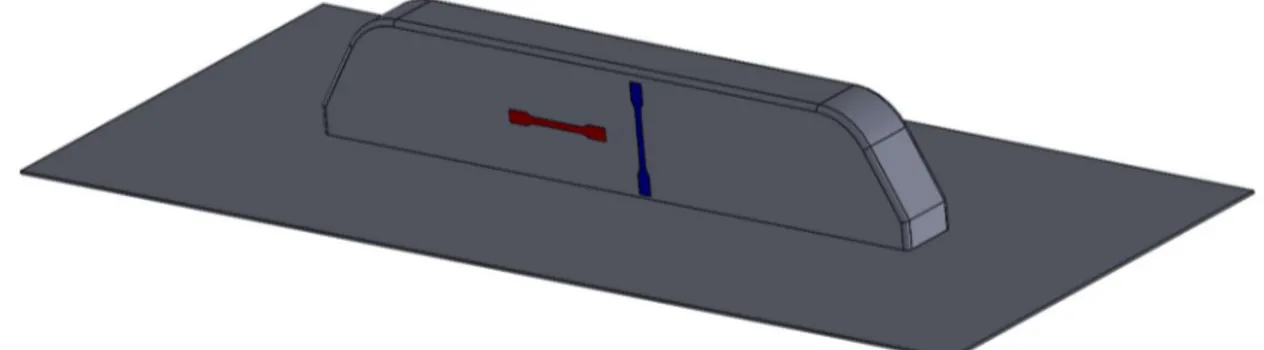
To identify and analyse the strain induced anisotropic material properties obtained in the formed samples, a number of tensile tests were done. The tensile specimens were cut in two directions from the side of the saddle, as shown in Figure 3.12. The X and Y directions correspond to the directions mentioned in section 3.1.2.

Figure 3. 12: Tensile specimens X(red) and Y(blue) directions

A total of 10 samples per direction were tested and the averaged results can be seen in Figure 3.13. As one can see, the material behaviour is altered depending on the stretch direction. As mentioned before in section 3.1.2, the material had stretched about 80% in Y-direction while the stretch in X-direction was negligible. As expected, the yield stress and the Young's modulus increase in the Y-direction due to strain induced effects.

Figure 3. 13: Average stress-strain curves in X and Y direction

3.2 Numerical model

3.2.1 FE-model

For the thermoforming simulation a 3D model of the saddle shaped geometry and the sheet were created in SolidWorks and exported to BETA ANSA for pre-processing. A first order quadrilateral shell mesh was generated for both the tool and the sheet with the properties as shown in Table 3.3.

Table 3. 3

*NIP = Number of through thickness Integration Points **ELFORM = Element formulation

In Figure 3.14 the FE-model is shown. The green coloured part is the sheet and the grey is the tool.

Figure 3. 14: FE-model

The element formulation used for the mesh of the sheet was a fully-integrated shell formulation based on Reissner-Mindlin kinematic assumption. This assumption takes mid-surface displacement and rotations into account to describe the shell deformation. It has 2x2 integration in the shell plane, as shown in Figure 3.15. An important additional feature is that the element has a linear through thickness strain which helps avoiding “Poisson’s locking” during bending deformation. The thickness stretch is governed by an artificial spring and provides degrees of freedom for loading and contact of the top or bottom surfaces of the shell, as shown in Figure 3.16. Hourglass type 8 was used since it is recommended for this element formulation in order to add warping stiffness. The thickness field was set to be continuous which is recommended for sheet metal forming [6].

Figure 3. 15: Element formulation number 26 [6]

Figure 3. 16: Properties of element formulation 26 [6]

3.2.2 Material data

During the thermoforming process the material temperature reaches 170±5°C which makes it behave like rubber. Those type of materials are often modelled using a viscoelastic or a hyperelastic material model [3]. In this work, the Ogden material model was used.

To simulate the process in a way that will reflect the reality, experiment data based on the tensile tests were used. From each sample a stress-strain curve was obtained. These curves were furtherly fitted using three-term polynomial functions in Matlab. For each set (5 samples for each temperature), a mean function was calculated (see Figure 3.17). Since the collected data only ranged until 125 °C, a relation between stress and temperature for each strain was made (see Figure 3.18). Assuming unchanged rheological material properties, the relation between stress-strain for a range of temperature between 125 and 170 °C was extrapolated. The stress-strain curves for all temperatures were plotted and are shown in Figure 3.19. A cross-section at 170 °C was then identified and plotted, as shown in Figure 3.20. This curve was then used as input to Hyperfit, which is a software for fitting of hyperelastic constitutive models based on experimental data [22]. A four-term Ogden model was fitted, as shown in Figure 3.21. The Ogden parameters μi and αi (Table 3.4) were then inputted to LS-DYNA keyword file.

Figure 3. 17: Average stress-strain curves at different temperatures

Figure 3. 19: Stress-strain-temperature relation

Figure 3. 21: Ogden curve fitting

Table 3. 4

Four-term Ogden model parameters

μ1 α1 μ2 α2 μ3 α3 μ4 α4 -0.12542 8547541 -1.51550 979316 3.87629 092586 0.14414580978 8 44.2608 895072 -0.00318 4331195 91 107.142 702462 -0.0054 9377255 864 3.2.3 Loadcase

In Figure 3.22, the contact set up is illustrated, where the blue coloured rigid body mesh, representing the tool, was set to be the master segment and the red coloured sheet mesh was set to be the slave. The contact type used was *AUTOMATIC_SURFACE_TO_SURFACE. The clamping was represented by setting boundary conditions (BC) on the outer nodes of the sheet, constraining all degrees of freedom (DOF), as shown in Figure 3.23. Temperature was indirectly applied to the sheet by using the Ogden parameters obtained from the extrapolated stress-strain curve at 170 °C. The pre-inflation and the vacuum were simulated by a distributed load on all elements except two rows neighbouring the boundary as shown in Figure 3.24. As can be seen in Figure 3.25, a prescribed rigid body motion with one degree of freedom, namely translation in the z-direction, was created to govern the raising of the tool. The magnitude and direction of the load applied to the sheet elements and the prescribed motion of the rigid body, were controlled by two manually defined curves shown in Figure 3.26 and 3.27.

Figure 3. 22: Contact definition

Figure 3. 23: Boundary conditions

Figure 3. 25: Prescribed rigid body motion

Figure 3. 27: Displacement curve

3.3 Verification and calibration of simulation

The formed samples were used to verify and later on calibrate the thickness distribution. This was done by cutting a thin strip of the middle section out of a "saddle" and measuring the thickness with a digital calliper at 50 points with a distance of 10mm, as shown in Figure 3.28 and Figure 3.29.

Figure 3. 29: Measurement points

Furtherly, the friction coefficient, between the tool and the sheet, in the simulation was adjusted so that the simulation results would agree with the measured data. The reason for using the friction coefficient to calibrate the simulation was that the actual value of this parameter was not determined.

After calibration the corresponding thickness distribution in the simulation was plotted together with the actual measurements, as shown in Figure 3.30.

Figure 3. 30: Prototype and simulation thickness distribution

From the above figure, one can see that there is a noticeable difference at point 26. This can be explained by the increase of the element size obtained during the simulation due to high strains in that area. The initial element length was 2.5mm, whereas in the final state it changed to approximately 7.5mm, which means that in y-direction the strain reached up to 200%. This makes it hard for the elements to follow the geometry of the tool limiting the level of strain compared to reality. The final thickness distribution according to the simulation is shown in Figure 3.31.

Figure 3. 31: Thickness distribution in simulation

3.4 Mapping the results to an undistorted mesh

To be able to use the obtained thickness distribution and altered material properties in a structural analysis, the results from the thermoforming simulation had to be mapped to a new undistorted mesh. This was done by using the built-in results mapping feature in BETA ANSA software. Since the nominal thickness of the plastic sheet is 4mm, the results were mapped on a 2mm offset surface from the tool geometry. The mapping was done using a 10mm search distance and the interpolation method chosen was "SHAPE FUNCTIONS". Furthermore, because of the importance that all elements get a mapped value, the extrapolate option was activated which creates results for elements that failed during mapping, based on neighbouring successful elements. With these parameters the overlap between the source and the target amounted to ~96%, which can be considered as sufficient enough.

As shown in Figure 3.32, the mapped thickness distribution is very alike the one obtained from LS-DYNA (Figure 3.31). To further illustrate the mapping results, a single element with ID 20517 was selected, as shown in Figure 3.33. The new thickness values for the four element nodes (THIC1, THIC2, THIC3 and THIC4) together with the material orientation PSI (BETA angle) are found in the element card, as shown in Figure 3.34.

Due to the fact that the Ogden model follows a hyperelastic behaviour, all strains in the final state of the thermoforming simulation are considered to be elastic. In reality though, when the material cools down below Tg, all deformations can be considered plastic. For this reason, a Python script that re-calculated an equivalent plastic strain based on the elastic strain tensor, was developed. The equation used in this is shown below (3.1) [18].

𝜀 = + (3.1)

Where the deviatoric strains are defined as in the equations 3.2.

𝑒 = − 𝜀 + 𝜀 − 𝜀 (3.2.b) 𝑒 = − 𝜀 − 𝜀 + 𝜀 (3.2.c)

𝛾 = 2𝜀 (3.2.d)

𝛾 = 2𝜀 (3.2.e)

𝛾 = 2𝜀 (3.2.f)

The calculated equivalent plastic strain for two through thickness integration points were mapped to the initial stress cards. Figure 3.35 shows the mapped strains on the target geometry and Figure 3.36 shows the initial stress card for a single element where EPS is the equivalent plastic strain values.

Figure 3. 32. Mapped thickness distribution

Figure 3. 34: Example element card

Figure 3. 35: Mapped equivalent plastic strain

3.5 Structural analysis

As a next step, the results from the thermoforming simulation were to be used in a structural analysis, with the aim to simulate the material behaviour with respect to thickness distribution as well as anisotropic strain hardening. The material model chosen for this purpose was the three-parameter Barlat, MAT_36 in LS-DYNA. This material model has the ability to include strain hardening and a dynamic Young's modulus based on equivalent plastic strain. To illustrate this, a tensile test simulation was done. The tensile specimen geometry used for the simulation was the same as in the tensile tests from the saddle geometry. The Young's modulus was determined by analysing the difference of the curves in Figure 3.13. From those curves, a linear function of effective plastic strain was derived, as expressed in equation 3.3. Young’s modulus in X and Y-direction were 1554 and 1849.5[MPa] respectively.

𝐸 = 369.375𝑒 + 1554 (3.3)

Additionally, the hardening curves in the directions 0˚, 45˚ and 90˚ were defined. This was done by assuming linear hardening and analysing the difference in yield stress from the experiments, leading to the linear expression 3.4. In the 90˚ direction, no hardening is assumed to occur since no strain was observed (equation 3.5). For the 45˚ angle, the weighting functions expressed in equation 3.6 were used, leading to the expression 3.7. The weighting functions are also shown graphically in Figure 3.37 [5]. The hardening curves in the directions of 0◦, 45◦ and 90◦ were plotted and shown in Figure 3.38. 𝜎 °_{= 7.6929𝑒 + 34.996 (3.4)} 𝜎 °_{= 34.996 (3.5)} 𝑤 (𝑎) = + cos(2𝑎) (3.6.a) 𝑤 (𝑎) = + cos 2(𝑎 + 90°) (3.6.b) 𝜎 °= 0.5𝜎 °+ 0.5𝜎 °= 3,84645𝑒 + 34.996 (3.7)

Figure 3. 37: Weighting functions [5]

Figure 3. 38 Hardening curves

Two simulations were done, one with no initial plastic strain and the other with an initial strain of 80%.

4 Findings and analysis

In this section, the implementation of the process described in the method and implementation section will be evaluated for a different geometry. The material used for the former simulation and the geometry in this section is the same, thus, focus is on the parts that differ. The new geometry that was simulated is the bottom part of a rooftop cargo carrier which is shown in Figure 4.1.

Figure 4. 1: Rooftop cargo carrier

4.1 Simulation of vacuum thermoforming

In this section, the geometrical and the thickness distribution results will be presented and analysed. It shall be noted that the initial thickness used for this case is 4.5 mm. All length units are in mm in the Figures below.

4.1.1 Geometrical results

Considering the forming results, the geometry after the simulation can be seen in Figure 4.2. As one can see, comparing Figure 4.1 with 4.2, the formed geometry followed the geometry of the tool in a good manner.

Figure 4. 2: Formed geometry in simulation

As for the mesh, the elements look as one would expect, meaning that for the most part they do not have unexpected distortions, as shown in Figure 4.3.

Figure 4. 3: Mesh after forming simulation

In some areas however, the elements seem to be unevenly stretched. These areas corresponded to the tool areas where the geometry was double curved and high strain levels were present. The strain paths follow the geometry in a reasonable way though. An example of this phenomena can be seen in Figure 4.4.

Figure 4. 4: Unevenly stretched mesh

A section view along the length of the rooftop cargo carrier is shown in Figure 4.5. One can see that the plastic sheet (green) followed the geometry of the tool (red) with high accuracy. In Figure 4.6, a close-up view of the red marked part in Figure 4.5 is shown, where a high accuracy can be seen for significantly stretched areas.

Figure 4. 5: Section view along the length of the component

Figure 4. 6: Close-up view

Another section view along the width of the rooftop cargo carrier is shown in Figure 4.7 and 4.8. The geometry in this direction includes more features and the formed sheet

did not follow the tool geometry as accurate as it did in the length direction. Still the result is sufficient for the purpose.

Figure 4. 7: Section view along the width of the component

Figure 4. 8: Close-up view

4.1.2 Thickness distribution results

The results of the thickness distribution of the plastic sheet is shown in Figure 4.9. It is noticeable that on the horizontal surfaces, the material is thicker than on the deep drawn ones. In Figure 4.10, the red marked area and the thinnest element are shown. A close-up view of the same area is illustrated in Figure 4.11.

Figure 4. 10: Thinnest area

Figure 4. 11: Thinnest element

Figure 4.12 shows the effective strain distribution of the plastic sheet. It is obvious that there is a direct correlation between the sheet thickness and the strain levels. The higher the strain, the thinner the elements become.

In Figure 4.13, the thinnest element together with the element that has the highest strain level are shown which illustrates that they are in the same area. This further confirms the relation between thickness and strain.

4.2 Results mapping

The results obtained from the thermoforming simulation were furtherly mapped on a mesh that was based on the geometry of the original CAD model. The mapped thickness distribution (EL.THICK) on the new mesh is shown in Figure 4.14. As one can see, this is in good agreement with the simulation results.

Figure 4. 14: Mapped thickness distribution

By running the developed script in Python, the mapping of the equivalent plastic strain (EL.EPS) was preceded by calculations based on the equations 3.1 and 3.2 in section 3.5. The results of the mapping are illustrated below in Figure 4.15 and are quite alike the ones obtained from the simulation.

4.3 Structural analysis

The results from the tensile test simulations that were described in section 3.6 are presented in this section. In Figure 4.16, the uniaxial stress in X-direction for the specimen with initial strain of 80% is shown. As expected, the maximum stress is 41.97 MPa, while in Figure 4.17, the specimen with no initial strain is shown and its maximum stress reaches 37.33 MPa.

Figure 4. 16: Tensile test simulation with initial strain of 80%

Figure 4. 17: Tensile test simulation with no initial strain

The stress-strain curves from both simulations are shown in Figure 4.18. As one can see, there is a difference in Young's modulus as well as in yield stress in agreement with the results from the tensile tests described in section 3.4. The plastic behaviour differs since linear plastic hardening was assumed in the simulations.

5 Discussion and conclusions

In this chapter discussions and conclusions of the method as well as of the findings are made.

5.1 Discussion of method

Obtainment of material data

The method for obtaining material data for ABS polymers at elevated temperatures resulted in some unforeseen complications with the equipment used. The internal height of the oven used was limited which resulted in that results only could be obtained to a certain extent of strain. The calibration of temperature in the oven was also sensitive, making it difficult and time consuming to stabilize the temperature. Since the openings in the oven could not fit the grips of the tensile test machine, custom made grips had to be produced for the specimen geometry. The material stress response in high temperatures was very low making it hard for the load cell used to register. For that reason, an extrapolated stress-strain curve was derived. For obtaining the Ogden parameters, the Hyperfit software was used, which facilitated this task tremendously. A major advantage of this software was that the curve fitting was visual, making it possible to assess the result before initiating time consuming simulations. To obtain data for the anisotropic material behaviour, tensile tests from formed components were done. The formed components were produced using a prototype thermoforming machine. The material of the tool was polyurethane with a relatively low thermal conductivity compared to the aluminium tool used in serial production. Furtherly, contrary to serial production, no additional cooling apart from the ambient air was applied. Those factors may be significant regarding the level of strain induced hardening.

All comparative tensile tests were done at constant strain rate which excluded possible strain rate effects on the stress response of the material.

Simulation

The software used for simulating the thermoforming process was LS-DYNA. This software has a wide variety of settings and parameters which made it time consuming to find a set up that converged and reflected reality sufficiently. The inflation and vacuum stages of the process were controlled using a distributed element load. This combined with the dynamic effects in the sheet made the simulation hard to calibrate. Problems regarding the contact between the tool and the sheet occurred. This was probably caused by a very low contact stiffness between the sheet and the tool. The effect of this was that the contact failed.

The advantages of using LS-DYNA for this work was that it is used by Thule for structural analysis and that it offers a wide variety of material models and flexibility in terms of simulation set up as well as processing results.

Ogden material model

This material model was chosen since it allowed up to an eight term hyperelastic function in LS-DYNA. This made it possible to get a material behaviour very close to

the one observed in the tensile tests. Another advantage was that this material model was included in the free version of Hyperfit software, which made it easy to calculate and visualise the result together with the values of the Ogden parameters. One drawback was that it was not possible to get a totally incompressible simulation by setting Poisson's ratio equal to 0.5. The reason was that this caused the timestep for the explicit analysis to reach zero. In contrary, if the Poisson's ratio was set to a low value, the timestep would increase substantially.

Mapping of results

This feature provided by BETA ANSA software appeared to be very useful and relatively easy to use. The results of the thermoforming simulation can be mapped on to a nondeformed mesh with an arbitrary size and geometry. For this project, it provided a great flexibility regarding search distance and interpolation method. The mapping results were also sufficiently accurate and the possibility to extrapolate results from nearby elements was also provided.

Structural analysis

It was quite difficult to select a material model that accounted for the altered material behaviour observed. One option was to develop a custom-made user defined material (UMAT). In agreement with the company it was decided to use an available material model instead, for time saving and simplicity reasons. In the chosen material model, the dynamic Young's modulus applied to all directions of each element, meaning that the possibility to have a material direction-driven Young's modulus was not possible. Although, each element can have a unique Young's modulus based on the strain levels obtained from the thermoforming simulation. The method altering the yield stress worked fine and was easy to set up.

Three-parameter Barlat material model

This material model was chosen for its flexibility to define the material behaviour based on an initial plastic strain. It offers a variety of plastic behaviours. In this case, linear plasticity was assumed to approximate the reality. To further increase the flexibility of this material model, it would have been of great value if the Young's modulus could be defined with three curves in the directions of 0°, 45° and 90°.

5.2 Discussion of findings

In this section the findings are discussed and evaluated with regard to the purpose and the research questions formulated.

Geometrical results

In the method and implementation, the correlation between strain and altered material properties was confirmed. Thus, before predicting the material properties, a simulation of the thermoforming process needed to be done. The geometrical results of this showed that it was possible, even though the geometries of the tool and the sheet did not completely conform. The conformity in the sections where the highest strains were observed, was considered sufficient.

Thickness distribution

The thickness distribution was of great interest since it accounts for the largest reduction of strength in the component. It has been shown that the thickness distribution can be simulated and the results shows a logical thickness change based on the strain levels. This is assumed valid based on the calibration done in the method and implementation. Any differences from reality could be explained by variations in production process, production equipment as well as environment.

Another source of error in the simulation can be related to the fact that extrapolated material data were implemented, for the reason that the equipment used was not well suited for the purpose. Since a hyperelastic material model was used, no strain rate effects were taken into account in the result. Lastly, the results can give a sufficiently accurate result if calibrated properly for each case.

Results mapping

One of the goals with this project was to be able to use thickness and strain distribution in a following analysis. For this purpose, a mapping of the results was done. The results from this are in good agreement with the results analysed in the post-processing software, LS-Prepost. Since all strains are considered to be elastic in the forming, a Python script converted these to plastic in result file. This script worked for a full-scale model as well.

Structural analysis

It has been shown that there is a possibility to use the plastic strain from the thermoforming simulation to get anisotropic material behaviour. Young's modulus as well as yield stress were altered elementwise based on their strain levels and direction. Young's modulus could not be altered for a single element in different directions though.

5.3 Conclusions

To conclude, it has been shown that it is possible to simulate the vacuum thermoforming process and predict the anisotropic material properties as well as the thickness distribution of the formed component. The anisotropic properties have, to some extent, been able to be used in a structural analysis. This makes it possible to do FE-analysis with an enhanced accuracy and in the long term, potentially reduce time and cost for new products to be developed.

The methodology presented can be further improved with accurate material data and calibration based on the real production process. Alternatively, generalized calibrations based on mathematical relations can be developed, taking friction coefficient as well as correct rheological material data into account.

The goals and the research questions of this project are considered fulfilled and answered. Thickness distribution, material properties and their directions can now be simulated and predicted with sufficient accuracy. The results can be used in a succeeding simulation of choice.

5.3.1 Further work

In this section, suggestions for further work based on problems encountered during this project are summarized.

Starting with the material model used in the thermoforming simulation, the material behaviour is more accurately simulated using viscoplastic models where strain rate effects are taken into account. The changes in temperature during the forming cycle can also be considered to more accurately correlate with reality. Moreover, in reality, the temperature distribution in the sheet is not uniform. This can be of importance for the thickness distribution and can be implemented in the simulation. Additionally, the heat transfer between the tool and the sheet has an influence on the material behaviour during the final stage of the process.

The possibility to include a directional dynamic Young's modulus would give closer to reality results and could thus be further investigated. In this work, the plastic behaviour of the material was assumed to be linear, which is not the case in reality. The possibility to use a non-linear plasticity model can thus be investigated. The validity of the thickness distribution of the full-scale rooftop cargo carrier model has not been confirmed either. Durability tests can be performed to check the validity of a structural analysis as well.

6 References

[1] Kutz Myer, (2011), Applied Plastics Engineering Handbook. Elsevier inc., ISBN 978-1-4377-3514-7.

[2] Laurence W. McKeen (2014), The Effect of Temperature and other Factors on Plastics and Elastomers, 3rd Edition. William Andrew, ISBN 978-0-323-31017-8. [3] Pierpaolo Carlone and Gaetano Salvatore Palazzo,Finite Element Analysis of the Thermoforming Manufacturing Process Using the Hyperelastic Mooney-Rivlin Model. In: M. Gavrilova et al. (Eds.): ICCSA 2006, LNCS 3980, pp. 794–803, 2006. [4] Interform specialist vacuum forming http://www.interform-uk.com/thermoplastic-vacuum-forming/vacuumform-process-grid2-02/ (Acc. 12 Mars 2018)

[5] Rolf Mahnken and Christian Dammann, Simulation of strain-induced anisotropy for polymers with weighting functions. In: Archive of applied mechanics (2014) 84:21-41

[6] André Haufe, Karl Schweizerhof, Paul DuBois, Properties & Limits: Review of Shell Element Formulations. Dynamore Developer Forum 2013 – Filderstadt/Germany – 24. September 2013

[7] Syed Ali Ashter (2014), Thermoforming of Single and Multilayer Laminates, William Andrew, ISBN: 978-1-4557-3172-5

[8] Y. Dong, R. J. T. Lin, D. Bhattacharyya, Determination of critical material parameters for numerical simulation of acrylic sheet forming. In: Journal of Materials Science (2005) 40(2):399-410

[9] P. Collins, J.F. Lappin, E.M.A. Harkin-Jones & P.J. Martin, Effects of material properties and contact conditions in modelling of plug assisted thermoforming. In: Plastics, Rubber and Composites (2000), 29:7, 349-359

[10] R.M. Hackett, Hyperelasticity Primer, Springer International Publishing Switzerland, ISBN 978-3-319-23273-7

[11] J. Chakrabarty, Applied Plasticity, Second Edition, Springer Science+Business Media, ISBN 978-0-387-77673-6

[12] Nam-Ho Kim, Introduction to Nonlinear Finite Element Analysis, Springer Science+Business Media, ISBN 978-1-4419-1745-4

[13] Miltiades C. Elliotis, A Finite Element Approach for the Elastic-Plastic Behavior of a Steel Pipe Used to Transport Natural Gas. In: Conference Papers in Energy volume 2013, Article ID 267095

[14] John O. Hallquist, LS-DYNA – Theoretical manual, Livermore Software Technology Corporation

[15] LS-DYNA – Keyword user's manual – Volume II – LS-DYNA R9.0, Livermore Software Technology Corporation

[16] D. Banabic, Sheet Metal Forming Processes, Springer-Verlag Berlin Heidelberg 2010

[17] J. Lubliner, P. Papadopoulos, Introduction to solid mechanics - An integrated approach. Second edition, Springer International Publishing

[18] DIANA - 9.4.4 User's Manual (2012)

https://dianafea.com/manuals/d944/Analys/node405.html (Acc. 11 May 2018) [19] Livermore Software Technology Corporation(2011-2018)

http://www.lstc.com/products/ls-dyna (Acc. 11 May 2018)

[20] Thule Group, http://www.thulegroup.com/en/about-thule-group (Acc. 14 May 2018)

[21] Philipp Hempel, Constitutive modeling of amorphous thermoplastic polymers with special emphasis on manufacturing processes, KIT Scientific Publishing, ISBN978-3-7315-0550-1