View of A Configural Perspective of Interindividual Differences in Intraindividual Change

Journal of Person-Oriented Research

Published by the Scandinavian Society for Person-Oriented Research Freely available at

http://www.person-research.org

A Configural Perspective of Interindividual Differences in

Intraindi-vidual Change

Alexander von Eye

, Wolfgang Wiedermann

2_{University of Missouri, Columbia}

Contact

voneye@msu.edu

How to cite this article

von Eye, A. & Wiedermann, W. (2016). A Configural Perspective of Interindividual Differences in Intraindividual Change. Journal of Person-Oriented Research, 2(1–2), 64–77. DOI: 10.17505/jpor.2016.07

Abstract: Lag analysis can be used to inspect stability and change of behavior over a pre-determined time interval, the

lag. In the analysis of metric variables, lag analysis is well known and used to identify such temporal effects as seasonal trends. In the analysis of categorical variables, the same can be done. Either approach can be employed in the analysis of both aggregated and individual data. In the domain of studying individual cells of contingency tables, that is, in configural analysis, only two sources exist in which lag analysis is discussed (von Eye, Mair, & Mun,2010;von Eye & Mun,2012). In this paper, we place the method of configural lag analysis in a person-oriented context and propose new variants for the comparison of individuals. Three approaches are considered. The first involves searching for configural types and antitypes separately for the comparison individuals. The second approach can be viewed parallel to two- or multiple group Configural Frequency Analysis. Both approaches are presented within a log-linear framework. Configural base models are specified for the original configural lag method as well as the extended comparative methods, and questions are defined that can be answered using configural lag analysis. The third approach allows researchers to test hypotheses concerning groups of cells. In an empirical example, data are analyzed from a study on the development of drinking behavior in alcoholics. Further extensions and alternative methods of analysis are discussed.

Keywords: Configural Frequency Analysis, person-oriented research, intraindividual change, lag analysis

Introduction

Configural Frequency Analysis (CFA; Lienert, 1969; von Eye & Gutiérrez-Peña,2004;von Eye et al.,2010) is used when researchers ask whether patterns of categorical vari-ables are observed at rates that differ from those expected under a particular probability model, the base model (von Eye,2004). Base models are specified so that only the ef-fects the researchers are interested in can be the reasons why individual patterns are observed at unexpected rates.

CFA is considered among the prime methods of analysis in person-oriented research (Bergman & Magnusson,1997; Bergman, Magnusson, & El-Khouri, 2003; Bergman, von Eye, & Magnusson, 2006;von Eye & Bergman,2003). It

has also been discussed in the context of Molenaar’s (2004) idiographic research (von Eye, Bergman, & Hsieh,2015). Interestingly, the methods of CFA developed so far (von Eye,2002a) are not only rooted in the family of methods of the Generalized Linear Model (predominantly used in a variable-oriented context). They are also methods that usu-ally result in statements about individuals or groups of in-dividuals(for the few approaches that represent exceptions to this rule, seevon Eye,2002a;von Eye et al.,2010). Idio-graphic and person-oriented research focus on the individ-ual. In fact, it is recommended that, in longitudinal, devel-opmental research, parameters be, before aggregation, esti-mated first at the level of individuals (Molenaar,2004;von Eye et al.,2015). In other words, developmental research,

which is mostly longitudinal, focuses first on intraindivid-ual changeand interindividual differences in intraindividual change(cf. Baltes, Reese, & Nesselroade,1977). Aggrega-tion, if desired, is then performed based on parameters, not raw scores.

There exist two configural approaches to analyze data from individuals with CFA. These are within-individual CFA (von Eye,2002a) and configural lag analysis (von Eye et al., 2010;von Eye & Mun,2012). The first element of person-oriented research, the description of individuals, can, thus, be accomplished using configural methods.

Before aggregation can be justified, individuals must be compared. Groups of individuals can be created only if the individuals’ scores differ only randomly from each other. Similarly, individuals can be declared members of pre-existing groups only if the individuals’ scores differ no more than randomly from scores that describe these groups. When systematic differences exist between profiles of an individual and a group, the membership of these indi-viduals and a group can be doubtful. Oddly, almost no con-figural methods have been proposed for the comparison of individuals (a first attempt can be found invon Eye & Mun, 2012). This type of methods would allow one to make de-cisions in the context of the second step of person-oriented analysis, the aggregation step. This step is performed to determine whether individuals differ in intraindividual de-velopment, that is, whether there exist interindividual dif-ferences in intraindividual change (von Eye & Mun,2012). In this article, we discuss existing configural methods for the description of individuals, and propose extending them with the goal of creating methods that allow one to make statements about interindividual differences in intraindi-vidual change.

Standard CFA analyzes groups of individuals. These are the individuals that constitute the entries in the cells of cross-classifications. To arrive at statements about individ-uals, the unit of analysis can no longer be the number of respondents in cells of tables. Instead, the unit of analysis must be the number of responses provided by an individ-ual. In other words, the cell counts in CFA of individuals represent the individual’s responses, not the number of in-dividuals. To arrive at statements about interindividual dif-ferences in intraindividual development, responses must be available from two or more individuals. This article is con-cerned with configural methods of analysis for this type of data.

This article is structured as follows. We first present a brief review of CFA (for more detail, see von Eye & Gutiérrez-Peña, 2004;von Eye, 2002a). We then review the method of configural lag analysis. In the central part of this article, we extend this method so that individuals can be compared. Three approaches will be discussed. For each of these three approaches, CFA base models are specified. The article concludes with an empirical data example and a discussion section.

Configural Frequency Analysis – A

Re-view

In this section, we start from the Generalized Linear Model (GLM;Nelder & Wedderburn,1972;McCullagh & Nelder, 1983). We then embed log-linear modeling and CFA in the context of the GLM, and discuss goals of analysis. The Gen-eralized Linear Model can be described as an extension of the General Linear Model. The latter is

µ =Xp_jβjxj,

whereµ is a vector of means, the xj ( j= 1, . . . , p) are

in-dicator variables, predictors, independent variables, or, in general, covariates, and the βs are the parameters whose values, usually, must be estimated. Now, let i be the in-dex for cases. Then, the systematic part of the GLM can be expressed as

E(Y_i) = µ_i=Xp

jβjxi j,

for, i_{= 1, . . . , N, the sample size, or, in matrix notation,} µ = X β,

where X is the model matrix, aka design matrix, andβ is the parameter vector. The generalization of the General Linear Model involves the following three elements. First, the element E(Y ) = µ is a convolution of the random com-ponent of the model,", and the systematic part, X β. In special cases, Y is independently normally distributed, with constant variance,σ2. Second, the systematic part of the model creates a linear predictorη,

η =X βjxj.

The third element connects the systematic and the ran-dom elements of the model by

ηi= g(µi).

The form g(.) is termed the link function. When g(.) is specified such that one obtains µ = η, this case is well known from linear regression analysis and analysis of vari-ance, the link function is the identity function. Any mono-tonic differentiable function can be considered as a link function. As discussed invon Eye and Mun(2013), for log-frequency models, the natural link function is the logarithm of the cell frequencies. One obtains

log(m) = X λ + ",

where m is the vector of observed cell frequencies,λ is the parameter vector," is the vector of model-specific residuals, and X is the matrix of covariates (predictors, independent variables, factors).

The goal of modeling is usually to arrive at a model that 1. reflects the underlying data generation mechanisms, 2. describes the data at hand satisfactorily, and

3. is parsimonious.

If a model possesses these characteristics, the residuals, "i, which indicate the discrepancies between the estimated

cell frequencies, ˆmi, and the observed cell frequencies, mi,

are random. The resulting statements are expressed in terms of relations among variables (effects). All of these are represented by the vectors of X , the design matrix.

From a person-oriented perspective, it is worth noting that these statements usually do not describe individuals or, in general, the data carriers. Most research follows the variable-oriented perspective. That is, variable rela-tions are targeted, and data carriers are random, replace-able with no more than random consequences for model fit or magnitude of parameters. In other words, if a sam-ple that is representative of some population is replaced by an independent, also representative sample, the resulting model will be largely the same.

In contrast, CFA targets individuals or groups of individ-uals. Using CFA, researchers aim at making statements that describe subgroups of data carriers, and the variables are no more than a random selection of measures. Other mea-sures of equal validity (reflecting the same construct of in-terest) are assumed to result in largely the same statements. To arrive at statements about individuals or groups of indi-viduals, CFA adopts a strategy that differs from that used for fitting models such as log-linear models. Specifically, researchers first specify those effects that are of interest. Examples of such effects are main effects, interactions, or planned contrasts, just as in ANOVA or log-linear model-ing. Based on these effects, researchers create the CFA base model. Most CFA base models are of the form given above for log-linear models, that is, log(m) = X λ + ". However, and this is specific to CFA, not all possible log-linear models qualify as CFA base models. Instead, log-linear (and other) models can be used as CFA base models only if they have the following characteristics (von Eye,2004):

1. it indicates the probability with which a pattern of cat-egories of the variables is expected to occur that span the cross-classification under study;

2. it takes all effects into account that are not of interest to the researchers; and

3. there is only one way to interpret discrepancies be-tween estimated and observed cell frequencies: they reflect the effects of interest.

If individual patterns of categories (these patterns are called configurations) are observed at unexpected rates, only the effects of interest can be the causes for these discrepancies. This strategy corresponds to a Popperian (1959) perspective, according to which rejecting false propositions eventually leads to correct statements. In con-trast to standard null hypothesis testing, however, and also in contrast to standard falsificationism, the strategy used in CFA results in a finite set of hypotheses, all of which the researchers can be interested in. The maximum num-ber of these hypotheses is given by the numnum-ber of cells in a cross-classification. Follow-up analyses can then be em-ployed to identify the specific effects that exist and cause

the discrepancies. Examples of follow-up analyses include variable-oriented log-linear modeling (von Eye et al.,2010) and person-oriented CFA (von Eye & Mair,2008b,2008a). Procedurally, CFA proceeds in the following steps (von Eye et al.,2010). First, a base model is specified that pos-sesses the above three characteristics. Most, but not all, CFA base models can be expressed as log-frequency models. Second, this model is estimated and model fit is evaluated. This part of the analysis is equivalent to standard log-linear model estimation (von Eye & Mun,2013). However, find-ing the best fittfind-ing model is not the goal of configural anal-ysis. Instead, one specifies a base model in the hope that it does not fit. Only if the base model fails to describe the data well, CFA continues. If the base model provides satisfactory model-data correspondence, none of the effects of interest exists, and the search for individual cells that deviate from expectancy is pointless.

In the third step, performed only after the base model fails, CFA null hypotheses are tested, usually for each cell of the cross-classification. The CFA null hypothesis states that, for each configuration, that is, in each cell, the difference between the expected and the observed frequencies is no greater than random. Specifically, the CFA null hypothesis states that

H₀: E_[mr] = ˆmr

where E[mr] is the expectancy for Cell r, where r

in-dexes the cells of a cross-classification, and ˆmr is the

esti-mated expected frequency for Cell r under a base model. Testing this null hypothesis results in one of three possible outcomes: CFA Type, Neither Type nor Antitype, and CFA Antitype. A cell constitutes a CFA type when the null hy-pothesis is rejected because the probability of mr is

BN,πr(mr− 1) ≥ 1 − α,

where N is the sample size,πris the probability of Cell r

under the base model, and mris the observed frequency of

cell r (below, we describe BN,πr as a binomial probability).

In other words, one can say that Cell r constitutes a CFA type when the null hypothesis is rejected because Cell r contains more cases than expected. Alternatively, the null hypothesis is rejected because

BN,πr(mr) ≤ α,

In other words, the null hypothesis can also be rejected because Cell r contains fewer cases than expected under a base model. In this case, Cell r is said to constitute a CFA antitype. When the null hypothesis prevails, the number of cases in Cell r is consistent with the base model.

Each of these tests is conducted under protection of the significance thresholdα. Protection is of great importance in CFA because of the large number of significance tests. In exploratory CFA, all cells of a table are subjected to a null hypothesis test. The most popular tests include the binomial testand the z-test. For the binomial test, let mr

denote the observed frequency of Cell r. Then, the exact tail probability of mr and more extreme frequencies is

Br(mr) = l X j=a N j ‹ pjqN− j,

where q= 1 − p, a = 0 if mr< ˆmrand a= mrif mr≥ ˆmr,

k= mr if a= 0 and l = N if a = mr. With the exception of

the rare cases in which the value p is known a priori, it is estimated from the sample. When the binomial test is used, CFA types emerge if

Br(mr− 1) = l X j=a N j ‹ pjqN− j≥ 1 − α,

and antitypes emerge, if

Br(mr) = l X j=a N j ‹ pjqN− j< α.

For the binomial test, the probabilities of the observed and each more extreme frequency are calculated and added to the total. There is no need to assume that any theoretical distribution is reasonably approximated. The binomial test is exact. This test is recommended when a sample is so small that the approximation properties of approximative tests are doubtful.

The most popular approximative test is the standard nor-mal z-test,

z= mr− N p pN pq .

Both, the binomial test and the z-test can be applied un-der any sampling scheme. More specifically, the multino-mial and the product-multinomultino-mial sampling schemes do not require that a different test than the binomial or the z-test be used. Other CFA tests are valid only under specific sam-pling schemes (for more detail on the protection ofα and for more CFA tests and their characteristics, seevon Eye, 2002a).

In the following sections, we discuss CFA of lags (cf.von Eye et al.,2010), the comparison of lag types and antitypes of individuals (von Eye & Mun,2012), and we propose ex-tensions of these methods.

CFA of Lags

In standard, cross-sectional data sets, the order of obser-vations usually carries no information. Whether Individual i’s data are listed before Individual j’s data or after is of no importance and has no implications for the results of data analysis. The same applies to longitudinal CFA. In this approach, however, the temporal order of data is of impor-tance. Consider, for example, the data in Table 1. The first row of Table 1 (labeled with “Day”) displays the number of beers an alcoholic has consumed on ten consecutive days.

For Days 2 through 10, we ask, how many beers the same individual had consumed on the day before. This informa-tion appears in the second row (“Day Before”) of data of Table 1. The data in the second row are called the lag-1 data. The number of beers consumed two days before ap-pears in the third row of data (“2 Days Before”). These data are called 2 data. Lag-2 data are the 1 data of lag-1 data. Expressed differently, lag-lag-1 data are shifted back

Table 1. Beer Consumption of an individual (artificial data)

Number of Beers Day 1 2 3 4 5 6 7 8 9 10 Day 2 2 5 3 5 5 3 1 5 4 Day Before 2 2 5 3 5 5 3 1 5 2 Days Before 2 2 5 3 5 5 3 1

one day, and lag-2 data are shifted back 2 days. Let Xt be

the observed data. Using the backshift operator, one creates lagged data. For example, lag-1 data are created by

B(xt) = Xt−1;

and lag-2 data are created by B(xt−1) = Xt−2.

The original data, xt, and the lagged data, Xt−i, can be subjected to various forms of statistical analysis. For exam-ple, one can ask whether the original data and the lag-7 data are correlated. In the example given in Table 1, this would correspond to the question whether particular days in a week are correlated with the number of beers this alco-holic individual consumes seven days before. Other ques-tions concern the detection of seasonal trends in tempera-ture or monthly trends in car sales.

Configural analysis allows one to answer these and other questions in the space of categorical variables, at the level of individual patterns. This is performed, in the simplest case, by crossing series that are shifted by a lag of l time points (here, j is used to index the original series of scores, and j0_{is used to index the shifted series of scores). To} ex-plain, let Xt, jbe category j of a categorical variable that was observed a point in time t. Let Xt−l, j0 be the same category

of the same variable, but shifted by a lag of l points in time. Then, Cell[Xt, j, Xt−l, j0] of the Xt× Xt−1cross-classification contains the number of observations for Category j at the first occasion that is followed by Category j0, at the lth oc-casion before.

In the context of configural analysis, there are two CFA base models that can be estimated for a Xt× Xt−l cross-classification. The first is the null model, log m = λ + ". The second model is that of variable independence. This is the main effect model, log m_{= λ + λ}X_{t+ λ}X_{t−l+ ". The}

interpretation of these models is discussed in the follow-ing section. When more lagged variables are considered or when information such as stratification or demographic variables is taken into account, more complex base models can be considered, e.g., prediction CFA. We now illustrate the use of lag CFA.

Data Example. To illustrate lag CFA, we use data from a longitudinal study of self-identified alcoholics (Perrine, Mundt, Searles, & Lester, 1995). A sample of alcoholic adult men provided every morning information about their drinking, as well as their subjective ratings of mood, health, and quality of the day before the interview. Here, we ask

whether associations exist between the number of standard size beers consumed on the same day of the week for con-secutive weeks, that is, for a lag of seven days. In other words, we set the shift operator to B(xt) = xt−7. We use the data from Respondent 3004. The range of the numbers of beers consumed by Respondent 3004 was wide. Even extremely high numbers are frequently reported. We nev-ertheless condensed this scale to range from 0= no beer consumed through 5= five or more beers consumed in one day. The main reason for condensing the scale this way is that other respondents reported fewer extreme numbers consumed at one occasion. Using the scale with scores from 0 through 5 makes it, therefore, easier to compare respon-dents. We will use these data for the other examples in this article as well. Respondent 3004 provided data for 742 con-secutive days. Because of the lag of 7 days, the lagged series contains data from 735 days. This respondent as well as all others started answering the phone interview questions on a Monday. Thus, the first reported day in the series is a Sunday.

The cross-classification of the original beer consumption figures with the ones from seven days before, was subjected to CFA. Because there are only two variables in the analysis, the number of possible base models is small. Based on the variables that span the cross-classification, that is, not con-sidering possible covariates or special effects and excluding the saturated model, there are four possible base models. These models are

1. log m= λ + "; this model is used for what was called Configural Cluster Analysis(Lienert & von Eye,1989); 2. log m= λ + λXt+ ";

3. log m= λ+λXt−7+"; types and antitypes from the

sec-ond and the third models are hard to interpret; they would indicate that there exist either the main effects of the variable whose main effect is not included or the interaction between the two series; considering that the two shifted series contain largely the same data, the first element of this interpretation seems implau-sible; therefore, we do not consider these models suit-able base models for lag CFA;

4. log m= λ + λXt+ λXt−7+ "; types and antitypes from

this base model indicate local associations between the lagged observations (Havránek & Lienert,1984). The first of these four models is the null model. It posits that there are only random local deviations from a uni-form distribution. This model would answer the question whether there are local density centers (types) or sparsely populated sectors (antitypes) in the space spanned by Xt

and Xt−7. Types and antitypes could be caused by main effects of either variable or the interaction Xt × Xt−7. In the present example, we ask whether there are local asso-ciations, regardless of possibly existing main effects. This question can be answered by estimating the fourth of the possible models. This is the model of variable indepen-dence, also called the main effect model. If this model fails and CFA results in types and antitypes, the question

concerning local associations can be considered answered based on the types and antitypes.

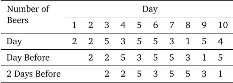
Thus, we estimated the model of independence of the two observation series. For the cell-wise CFA tests, we set the significance level to α = 0.05, and we used the z-test and theHolland and Copenhaver(1987)α protection. Ta-ble 2 displays the results of this analysis.

Table 2. First order CFA of beer consumption of Respondent 3004

with a lag of seven days.

Configuration Xt Xt−7 m mˆ z p 0 0 85.00 25.165 11.9279 .000000 T 0 1 15.00 5.921 3.7311 .000095 T 0 2 16.00 6.661 3.6184 .000148 T 0 3 8.00 5.181 1.2385 .107765 0 4 3.00 7.771 -1.7116 .043487 0 5 9.00 85.301 -8.2614 .000000 A 1 0 18.00 5.921 4.9639 .000000 T 1 1 3.00 1.393 1.3613 .086708 1 2 5.00 1.567 2.7419 .003055 1 3 2.00 1.219 .7073 .239685 1 4 .00 1.829 -1.3522 .088148 1 5 4.00 20.071 -3.5872 .000167 A 2 0 13.00 6.846 2.3519 .009340 2 1 7.00 1.611 4.2461 .000011 T 2 2 1.00 1.812 -.6034 .273134 2 3 1.00 1.410 -.3449 .365070 2 4 5.00 2.114 1.9846 .023595 2 5 10.00 23.207 -2.7415 .003058 3 0 9.00 5.551 1.4639 .071614 3 1 3.00 1.306 1.4821 .069151 3 2 2.00 1.469 .4377 .330790 3 3 3.00 1.143 1.7372 .041176 3 4 2.00 1.714 .2182 .413630 3 5 11.00 18.816 -1.8019 .035779 4 0 3.00 7.956 -1.7572 .039445 4 1 .00 1.872 -1.3683 .085617 4 2 .00 2.106 -1.4512 .073355 4 3 3.00 1.638 1.0641 .143645 4 4 3.00 2.457 .3463 .364553 4 5 34.00 26.970 1.3537 .087922 5 0 8.00 84.561 -8.3257 .000000 A 5 1 4.00 19.897 -3.5638 .000183 A 5 2 12.00 22.384 -2.1948 .014091 5 3 11.00 17.410 -1.5361 .062251 5 4 29.00 26.114 .5647 .286140 5 5 393.00 286.635 6.2825 .000000 T

Note.T= Type, A = Antitype;

The overall goodness-of-fit LR-X2_{for the base model of} the cross-classification in Table 2 is 498.81. For d f = 25, this value indicates poor fit (p < 0.001). We reject the base model and proceed to the CFA tests. The results of these tests are given in Table 2. For illustration purposes, we just interpret the two most extreme types and the two most extreme antitypes, where ’extreme’ is based on the magnitude of the z-statistic.

Type 0 0: The most extreme type is one of stability of stay-ing sober on correspondstay-ing days of the week. More often than expected under the assumption of independence be-tween the reports a week apart, Respondent 3004 reported that he consumed no beer at all on two corresponding days of the week. This pattern occurred 85 times, but the base model led one to expect only 25.17 times.

Type 5 5: The second-most extreme type is one of sta-bility of drinking excessively on corresponding days of the week. More often than expected under the assumption of independence between the reports a week apart, Respon-dent 3004 reported consuming five beers or more on two corresponding days of the week. This occurred 393 times but had been expected to occur on only 286.64 days.

Antitype 5 0: The most extreme antitype suggests that drinking excessively after having consumed nothing seven days before is extremely unlikely. This pattern occurred eight times, but had been expected to occur 84.56 times.

Antitype 0 5: This is the reverse pattern to Antitype 5 0. It suggests that drinking nothing after having consumed excessively seven days before is extremely unlikely as well. This pattern occurred nine times, but it had been expected to occur 85.30 times.

From these results, we draw the conclusion that Respon-dent 3004’s beer consumption behavior is very predictable from one day to the same day, one week later. CFA results suggest that patterns of heavy drinking, patterns of staying sober, and patterns shifting from drinking to staying sober and vice versa occur at extreme rates. However, not all patterns deviate from expectancy. The number of extreme patterns is, from a CFA perspective, not out of the ordinary. The patterns that are well represented by the model of in-dependence of drinking from one day to the corresponding day of the following week suggest that, in most cells of the table, there is independence. CFA tells the user where, in the table, local associations exist.

There are many other questions than the one concerning local associations. For example, one can ask whether there are patterns of multiple types or patterns of multiple anti-types for Respondent 3004. We will come back to this ques-tion later, in this article. One could also ask whether this respondent changes his drinking behavior over the course of the 3.5 years that he provided data for. In the next sec-tion, we focus on a third quessec-tion, also within the context of person-oriented research. This is the question concerning the comparison of two respondents.

Comparing Two Individuals’ Lag

Pat-terns

In the last section, we illustrated that CFA can well be used to identify longitudinal behavioral patterns for the individ-ual (cf.von Eye et al.,2010;von Eye & Mun,2012). In this section, we illustrate that CFA can also be used to compare individuals in such patterns. We present two approaches. The first involves estimating the same base model for two or more individuals, in separate runs, and then heuristically compare the resulting type and antitype patterns. The

sec-ond approach involves performing a variant of 2-group CFA to the comparison individuals.

These two approaches help answer different questions. The first approach runs individual-specific CFAs. Results indicate whether the comparison individuals’ behavior ex-hibits local associations. These associations may or may not exist, regardless of the patterns that describe the respec-tive other individuals. The second approach answers the question whether comparison individuals differ in particu-lar configurations, regardless of whether this configuration constitutes a type or antitype (or nothing) for one or both of the individuals.

In this section, we illustrate both approaches. We begin with the first. It simply involves running CFAs as illustrated in the last section, for two or more individuals. For the purpose of comparison, the base models, the test used for the CFA hypotheses, and the protection ofα in the multiple CFA runs must be exactly the same.

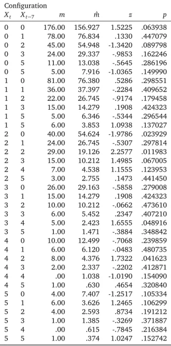
Data Example. In this data example, we use data from the same study as in the first example. We use data from respondent 3000. As for Respondent 3004, we estimate the base model of variable independence, use the z-test, and apply the Holland-Copenhaver strategy of α-protection. The results of this analysis appear in Table 3.

The overall goodness-of-fit LR-X2for the base model of the cross-classification in Table 3 is 35.36. For d f = 25, this value indicates solid fit (p= 0.08). We retain the base model and see no point in proceeding to the CFA tests. In-deed, the results in Table 3 suggest that not a single cell constitutes a type or an antitype. The drinking habits of Re-spondent 3000 are unpredictable when one compares cor-responding days of the week.

This result and the one reported in Table 2 are in accor-dance with the ones presented by von Eye and Bergman (2003), for the same individuals. The authors had calcu-lated autocorrelations for these two respondents, over a wide range of lags. The results of that analysis suggested that the two respondent differ in volume and predictability of beer consumption.

The interpretation of the CFA results in Table 3, in com-parison with those in Table 2, is straightforward. Whereas Respondent 3004 is well predictable in a number of pat-terns, Respondent 3000 shows no local associations at all, for a lag of seven days. Note, however, that the present re-sults may be specific to the chosen lag of one week. von Eye and Bergman(2003) showed that, for lags that only cover drinking patterns from one day to the next, Respondent 3000 is well predictable. The visual comparison of z-values indicate where individual-specific local associations exist (see Figure 1), and it becomes evident that such associa-tions do exist for Respondent 3004 but not for Respondent 3000. In the next section, we discuss how to statistically compare these two respondents with the aim of identifying those lag patterns in which the two respondents differ.

Table 3. First order CFA of beer consumption of Respondent 3000

with a lag of seven days.

Configuration Xt Xt−7 m mˆ z p 0 0 176.00 156.927 1.5225 .063938 0 1 78.00 76.834 .1330 .447079 0 2 45.00 54.948 -1.3420 .089798 0 3 24.00 29.337 -.9853 .162246 0 5 11.00 13.038 -.5645 .286196 0 5 5.00 7.916 -1.0365 .149990 1 0 81.00 76.380 .5286 .298551 1 1 36.00 37.397 -.2284 .409652 1 2 22.00 26.745 -.9174 .179458 1 3 15.00 14.279 .1908 .424323 1 5 5.00 6.346 -.5344 .296544 1 5 6.00 3.853 1.0938 .137027 2 0 40.00 54.624 -1.9786 .023929 2 1 24.00 26.745 -.5307 .297814 2 2 29.00 19.126 2.2577 .011983 2 3 15.00 10.212 1.4985 .067005 2 4 7.00 4.538 1.1555 .123953 2 5 3.00 2.755 .1473 .441450 3 0 26.00 29.163 -.5858 .279008 3 1 15.00 14.279 .1908 .424323 3 2 10.00 10.212 -.0662 .473610 3 3 6.00 5.452 .2347 .407210 3 4 5.00 2.423 1.6555 .048916 3 5 1.00 1.471 -.3884 .348842 4 0 10.00 12.499 -.7068 .239859 4 1 6.00 6.120 -.0483 .480735 4 2 8.00 4.376 1.7322 .041623 4 3 2.00 2.337 -.2202 .412871 4 4 .00 1.038 -1.0190 .154090 4 5 1.00 .630 .4654 .320840 5 0 4.00 7.407 -1.2517 .105334 5 1 6.00 3.626 1.2465 .106299 5 2 4.00 2.593 .8734 .191212 5 3 1.00 1.385 -.3269 .371887 5 4 .00 .615 -.7845 .216384 5 5 1.00 .374 1.0247 .152742

Statistically Comparing Lag Patterns

In the simplest case, there is one additional variable in a configural lag comparison, the variable that indicates the comparison units. Let this variable be labeled P. Let the two lag variables be labeled Xt and Xt−l. For these three variables, the following base models are conceivable (again excluding models with covariates or special effects, and also excluding models that are as hard to interpret as the second and the third, above):

1. log m= λ + ",

2. log m= λ + λXt+ λXt−lλP+ ", and

3. log m= λ + λXt+ λXt−l+ λP+ λXt,Xt−l_.

It should be noted that many other log-linear mod-els could be considered for these three variables,

includ-ing hierarchical, non-hierarchical, and nonstandard models (Mair & von Eye,2007). None of these, however, qualifies as a CFA base model (cf. the criteria for CFA base models listed above; von Eye,2004). Therefore, we only discuss these three models. The first of the three base models is, as before, the null model. It allows one to answer the ques-tion where, in the cross-classificaques-tion of P, Xt, and Xt−l, observed frequencies deviate significantly from the grand mean of frequencies. As in the first two examples, how-ever, we focus on local associations.

Therefore, we are more interested in the second and the third base models. The second is that of variable indepen-dence. If it fails and types and antitypes emerge, we know that local associations exist. These associations may rep-resent different patterns for the comparison units. That is, they can be respondent-specific. However, they do not al-low us to answer the question concerning the differences between the comparison units. To answer this question, we need the third base model. It corresponds to that of 2-group CFA. It includes the association between the com-parison variables. However, it posits that no qualification of this association is needed that is related to the comparison units. In other words, this model posits that the associa-tion between the comparison variables is the same across all comparison units.

If this model fails and types and antitypes emerge, there is only one reason for their existence: Individual patterns differ across the comparison units. This could have been captured only by the three-way interaction among P, Xt,

and Xt−l and the two two-way interactions P× Xt and

P× Xt−7. These terms are not part of the base model. They were omitted for two reasons. First, including these terms and specifying the base model such that it is hierarchical would result in a saturated model. Here, we are not inter-ested in this model because we focus on individual pairs of cells (when there are two comparison units; when there are more, the number of cells in each comparison increases; see von Eye, 2002a). Second, finding that the three-way interaction is significant will not allow one to answer the CFA-specific question of where exactly in the space of the three variables P, Xt, and Xt−ldifferences are located. This question can be answered only with CFA.

In general, the model to be used for the comparison of lagged information from two or more individuals contains the following terms:

1. all main effects of all variables in the analysis; 2. all possible interactions among the variables used for

comparison; the model is, thus, saturated in the com-parison variables;

3. all possible interactions among the variables used to classify the comparison units; usually, there is only one such variable; however, there are instances in which more than classification variable is used (e.g., age, gender, and extraversion); in these instances, the model is saturated in the classification variables as well.

Including all these terms implies first that this base model posits that the comparison variables are independent of the

Figure 1. Comparison of Type/Antitype-configurations for the two individuals. The solid lines refer to the Bonferroni-adjusted critical

z-values.

comparison units. If this proposition fails, CFA allows one to determine the patterns of the comparison variables in which comparison units differ from each other. The sec-ond implication is that any of the comparison variables and any combination of comparison variables can be associated with the classification variables. This issue will be taken up again later, in this article. We now proceed to the real-world data example.

Data Example. In the following example, we continue the analysis of lagged drinking behavior patterns of respon-dents 3000 and 3004. We estimate the above third base model, which is, in the present example,

log m= λ + λXt+ λXt−7+ λP+ λXt,Xt−7

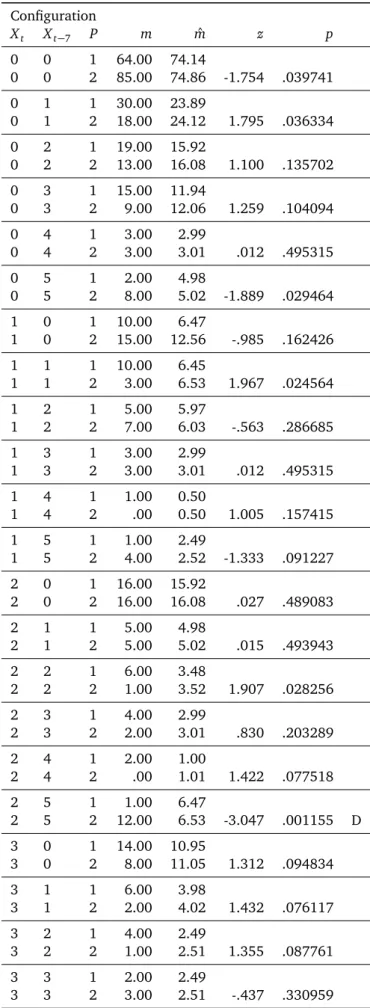
where P distinguishes between Respondents 3000 and 3004, and Xt, and Xt−l represent the original drinking variables and the ones after invoking the shift operator B(xt) = xt−7. For the CFA, we use, as in the first examples, the z-approximation of the binomial test, and, to protect α, we employ the Holland-Copenhaver procedure. Table 4 displays the results of the comparison of Respondents 3000 and 3004.

The overall goodness-of-fit LR-X2_{for the base model of} the cross-classification in Table 2 is 1014.16. For d f = 35, this value indicates poor fit (p< 0.001). We reject the base model and proceed to the CFA tests. The results of these tests are given in Table 4.

Table 4 is structured so that the comparison pairs are presented in one cell each. For example, in the first cell, we compare Respondents 3000 and 3004 (labeled as 1 and 2) in Pattern 0 0. For each comparison, there is only one

test. This implies that the protected significance thresh-old is less extreme than when each cell is subjected to a CFA test. Therefore, 2-group CFA of lagged data has more statistical power than the corresponding CFA that performs one test per pair of observed and expected cell frequen-cies. Table 4 shows nine discrimination types. This indi-cates that Respondent 3000 differs from Respondent 3004 in nine lagged drinking patterns. To illustrate, we interpret the two most extreme discrimination types, where ’extreme’ is, as above, based on the magnitude of the test statistic.

Discrimination Type 5 5 1/ 5 5 2: As shown in Table 2, Pattern 5 5 constituted a lagged drinking type in the sep-arate analysis of Respondent 3004. Here, we see that the two respondents differ extremely in this pattern. Respon-dent 3004 reported having consumed five or more beers on corresponding days of consecutive weeks 393 times. In contrast, Respondent 3000 reported this pattern only 10 times.

Discrimination Type 5 0 1/ 5 0 2: Pattern 5 0 also stood out in the separate analysis of Respondent 3004. There, it constituted an antitype. Here, we see that the two respon-dents differ in this pattern as well. Whereas Respondent 3000 switched 218 times from drinking nothing to drink-ing 5 or more beers on corresponddrink-ing days of two weeks, Respondent 3004 did this only nine times. It is interest-ing to note that Pattern 0 5, which constituted an antitype in the separate analysis of Respondent 3004 as well, does not emerge as extreme in the present analysis. This pattern occurs equally rarely for both respondents.

From the results in Table 4, we conclude that

• patterns that constitute types or antitypes in the sepa-rate analysis of individuals do not necessarily also con-stitute discrimination types in the comparison of

indi-viduals; examples include Patterns 0 5, 5 2, and 5 3; • patterns that fail to constitute types or antitypes in

the separate analysis of individuals, can constitute dis-crimination types nevertheless; examples include Pat-tern 4 5.

In sum, results from the separate analysis of individuals are not predictive of results from the statistical comparison of the same individuals. Reasons for this are (1) that the base models for these two configural analyses take different information into account, and (2) that the base models are specified so that they speak to different questions.

Patterns of Patterns: Compound Patterns

directly compare individuals but to also answer questions concerning individual cells and groups of cells. In this sec-tion, we discuss questions concerning groups of cells – also a first in the context of CFA of lagged data. Specifically, one can ask whether the cells in a selected group of cells jointly stand out. If this question is answered in the affirmative, these cells constitute a joint CFA type or a joint CFA anti-type. When two or more individuals are compared, these joint types_{/antitypes indicate where the comparison units} differ in the sense that the total number of observations in the cells in a group of cells is significantly larger/smaller than expected for one of the comparison units. This inter-pretation results from the characteristics of the base model. The only terms not included in the base model are the in-teractions between the comparison variables and the com-parison units. Therefore, if groups of cells stand out, these interactions are the only possible causes.

A number of test statistics has been proposed that allow one to test the null hypothesis that a group of cells jointly has an occurrence rate that deviates from the expected (cf. Darlington & Hayes,2000;von Eye,2002a). They all take into account that the test statistics for individual cells, e.g., X2 _{values or z scores, cannot simply be averaged or} summed because the resulting scores would not approxi-mate a known sampling distribution closely enough. Each of these statistics can be used to test the present null hy-pothesis. However, we consider Stouffer’s (Stouffer, Such-man, DeVinney, Star, & Williams,1949) Z-statistic as being most suitable. The main reasons for this choice are (1) that Stouffer’s Z is as powerful as the other statistics, and, more important in the present context, (2) that it can be used for one-sided testing. Z approximates the standard normal, that is, a symmetrical distribution.

The statistic can be described by

Z= X i mi− N ˆpi q N ˆp_iqˆ_i ! /pnc g= Pt izi p_n c g

where i goes over the cells that constitute the group un-der examination, nc gis the number of cells in the group, p

is estimated asmˆi

N, and ˆq= 1 − ˆp.

Table 4. 2-Group CFA for the comparison of beer consumption of

Respondents 3000 and 3004, with a lag of seven days (Respon-dent 3000 labeled as 1, Respon(Respon-dent 3004 labeled as 2).

Configuration Xt Xt−7 P m mˆ z p 0 0 1 64.00 74.14 0 0 2 85.00 74.86 -1.754 .039741 0 1 1 30.00 23.89 0 1 2 18.00 24.12 1.795 .036334 0 2 1 19.00 15.92 0 2 2 13.00 16.08 1.100 .135702 0 3 1 15.00 11.94 0 3 2 9.00 12.06 1.259 .104094 0 4 1 3.00 2.99 0 4 2 3.00 3.01 .012 .495315 0 5 1 2.00 4.98 0 5 2 8.00 5.02 -1.889 .029464 1 0 1 10.00 6.47 1 0 2 15.00 12.56 -.985 .162426 1 1 1 10.00 6.45 1 1 2 3.00 6.53 1.967 .024564 1 2 1 5.00 5.97 1 2 2 7.00 6.03 -.563 .286685 1 3 1 3.00 2.99 1 3 2 3.00 3.01 .012 .495315 1 4 1 1.00 0.50 1 4 2 .00 0.50 1.005 .157415 1 5 1 1.00 2.49 1 5 2 4.00 2.52 -1.333 .091227 2 0 1 16.00 15.92 2 0 2 16.00 16.08 .027 .489083 2 1 1 5.00 4.98 2 1 2 5.00 5.02 .015 .493943 2 2 1 6.00 3.48 2 2 2 1.00 3.52 1.907 .028256 2 3 1 4.00 2.99 2 3 2 2.00 3.01 .830 .203289 2 4 1 2.00 1.00 2 4 2 .00 1.01 1.422 .077518 2 5 1 1.00 6.47 2 5 2 12.00 6.53 -3.047 .001155 D 3 0 1 14.00 10.95 3 0 2 8.00 11.05 1.312 .094834 3 1 1 6.00 3.98 3 1 2 2.00 4.02 1.432 .076117 3 2 1 4.00 2.49 3 2 2 1.00 2.51 1.355 .087761 3 3 1 2.00 2.49 3 3 2 3.00 2.51 -.437 .330959

Table 4. (continued) Configuration Xt Xt−7 P m mˆ z p 3 4 1 1.00 1.99 3 4 2 3.00 2.01 -.992 .160648 3 5 1 1.00 5.97 3 5 2 11.00 6.03 -2.882 .001976 4 0 1 17.00 9.95 4 0 2 3.00 10.05 3.174 .000753 D 4 1 1 13.00 6.47 4 1 2 .00 6.53 3.639 .000137 D 4 2 1 5.00 4.98 4 2 2 5.00 5.02 .015 .493943 4 3 1 3.00 2.49 4 3 2 2.00 2.51 .459 .323224 4 4 1 3.00 2.99 4 4 2 3.00 3.01 .012 .495315 4 5 1 1.00 14.93 4 5 2 29.00 15.07 -5.139 .000000 D 5 0 1 218.00 112.96 5 0 2 9.00 114.04 15.171 .000000 D 5 1 1 101.00 52.25 5 1 2 4.00 52.75 9.876 .000000 D 5 2 1 79.00 44.29 5 2 2 10.00 44.71 7.594 .000000 D 5 3 1 36.00 23.39 5 3 2 11.00 23.61 3.740 .000092 D 5 4 1 17.00 25.38 5 4 2 34.00 25.62 -2.388 .008463 5 5 1 10.00 200.54 5 5 2 393.00 202.46 -22.301 .000000 D

Note.D= Discrimination Type; Discrimination types result from the comparison of the two frequencies in the same row pair, relative to the total sample sizes for the comparison respondent.

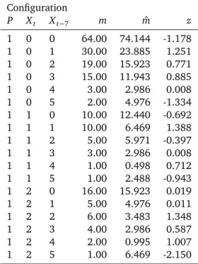
Data Example. In the following data example, we con-tinue the analysis of the data obtained from Respondents 3000 and 3004. The base model used for the comparison of the predictability of beer drinking of these two respondents via 2-group CFA of lagged data yields the expected cell fre-quencies given in Table 5 (these are also the expected cell frequencies that underlie the analyses for Table 4).

Table 5 does not display any tests for types or antitypes. These would reflect the results from examining individual cells. Here, we ask questions concerning groups of cells. Specifically, we ask the following two questions:

1. Considering that Respondent 3000 drinks, on average, less beer than Respondent 3004, is it more likely than one would expect under the assumption that there are no interindividual differences in the effects that describe the data in Tables 4 and 5 that Respondent

3000, in comparison with Respondent 3004, exhibits, on corresponding days of the week, drinking patterns in which he combines drinking fewer beers before or after he consumed large numbers of beers on the cor-responding day the week before (or after)?

2. In turn, considering that Respondent 3004 drinks, on average, more beer than Respondent 3000, is it partic-ularly less likely than one would expect under the as-sumption that there are no interindividual differences in the effects that describe the data in Tables 4 and 5 that Respondent 3004 exhibits, on corresponding days of the week, drinking patterns in which he combines drinking fewer beers before or after he consumed large numbers of beers on the corresponding day the week before (or after)?

These two questions may sound similar. However, in the first question we consider the drinking pattern of Respon-dent 3000, relative to the drinking of ResponRespon-dent 3004. In contrast, in the second question, we consider the drinking pattern of Respondent 3004, relative to the drinking of Re-spondent 3000. These relations usually do not correspond. The cells that speak to the first question are 1 5 0, 1 5 1, 1 5 2, 1 5 3, and 1 5 4 (see Table 5). The cells that speak to the second question are 2 5 0, 2 5 1, 2 5 2, 2 5 3, and 2 5 4 (see also Table 5). Inserting into the formula for Z to answer the first question, we obtain

Z= (9.884+6.744+5.216+2.608−1.663)/p5= 10.192. This value is more extreme than compatible with the one-sided 0.05 significance threshold of 1.645 (p< 0.01), and we conclude that Respondent 3000 does indeed more of-ten than expected return to drinking nothing after having consumed at least one beer on the corresponding day of the week before. The five configurations 1 5 0, 1 5 1, 1 5 2, 1 5 3, and 1 5 4 thus constitute a joint CFA type. This is in contrast to Respondent 3004.

This statement can be formulated even more specifically after answering the second question. Inserting into the for-mula for Z to answer this question, we obtain

Z= (−9.836−6.712−5.191−2.596+1.655)/p5_{= −10.143,} a value that also exceeds the critical one-sided value for a significance threshold ofα = 0.05 (p < 0.01). We conclude that it is not only more likely that Respondent 3000 returns to drinking nothing from having consumed one or more beers on the corresponding day the week before, it is also less likely than expected that Respondent 3004 does the same. The five configurations 2 5 0, 2 5 1, 2 5 2, 2 5 3, and 2 5 4 thus constitute a joint CFA antitype. Please note that, in both cases, the hypotheses are one-sided. This was one of the reasons why we selected Stouffer’s test.

Base Models and Interpretation of Joint Types and An-titypes. In the last section, we discussed joint types and antitypes for configural lag analysis of interindividual dif-ferences in intraindividual change of drinking patterns. We examined the interplay of the three variables P, Xt, and

Xt−7 from a configural, person-oriented perspective. The interpretation of the joint type and the joint antitype was based on omitting all interactions from the base model that would include Variable P. That is, we used the base model log m = λ + λXt + λXt−7+ λP + λXt,Xt−7_{. This base model}

proposes that neither the original series nor the one that re-sults from invoking the backshift operator B(xt−1) = xt−7is respondent-specific, and neither is the interaction between the two series. There are three interactions that involve P. These are the interactions[Xt, P], [Xt−7, P], and [Xt, Xt−7,

P]. Omitting all three of them is in line with the rules set up for 2- or more-group CFA.

This decision, however, may be discussable, in the present context. For example, it may be the case that[Xt−7,

P] exists when [Xt, P] also exists. Differences will solely be

due to the size of the lag because the second series, Xt−7, will be shorter than the first by a number of days that is given by the size of the lag. Therefore, one of the interac-tions may be redundant, given the other. Because of this redundancy, the three-way interaction plus one of the two-way interactions may be sufficient for the interpretation of resulting joint types and joint antitypes. Specifically, and extending the series of models considered by (von Eye & Mun,2012), four base models are conceivable:

1. Model 1: log m_{= λ + λ}X_{t+ λ}X_{t−7+ λ}P_{+ λ}X_t,Xt−7_{; this is}

the standard base model used in 2-group CFA, it was used for the analyses in Tables 4 and 5; this model pro-poses that the comparison respondents differ in their original and lagged series of scores;

2. Model 2: log m= λ+λXt+λXt−7+λP+λXt,Xt−7+λXt,P_;

this is the base model that searches for types and an-titypes under the assumption that the first of the two series is not specific to the comparison individuals; this model considers the first of the two-way interactions redundant;

3. Model 3: log m_{= λ+λ}X_t+λX_t−7+λP_+λX_t,Xt−7+λXt−7,P_;

this is the base model that searches for types and an-titypes under the assumption that the second of the two series is not specific to the comparison individu-als; this model considers the second of the two-way interactions redundant; and

4. Model 4: log m= λ+λXt+λXt−7+λP+λXt,Xt−7+λXt,P+

λXt−7,P_{; this is the model of all two-way interactions; it}

is parallel to a logit model (for a comparison of logit models and CFA, seevon Eye, Mair, & Bogat,2005); in standard modeling, this model is of interest when one assumes that the three-way interaction does not make an important contribution to explaining the frequency distribution in the cross-classification; from the per-spective of a configural analysis of interindividual dif-ferences in intraindividual change, however, this may be the most important effect; this model suggests that the two comparison respondents differ in the relation between the original and lagged series of scores. Indeed, estimating these four base models yields dif-ferent goodness-of-fit results. Specifically, we obtain, for Model 1, LR-X2= 1041.16 (d f = 35; p < 0.01), for Model

2, LR-X2_{= 1041.04 (d f = 30; p < 0.01), for Model 3,}

LR-X2= 250.24 (d f = 30; p < 0.01), and for Model 4, LR-X2 = 94.39 (d f = 25; p < 0.01). None of these models fits, and one can expect types and antitypes to emerge. How-ever, whereas the difference between the first two models is minimal, the difference between the first and the third is significant. We can conclude that the interaction[Xt, P]

does make a strong contribution to the emergence of types and antitypes. The difference between Models 1 and 4 is significant as well. Considering that Model 4 is rejected, we conclude that the three-way interaction does also play an important role in the explanation of the frequency distribu-tion in Table 4, and may be the main cause for discrimina-tion types to emerge (for more detail on the comparison of log-linear models, see (von Eye & Mun,2013)).

Note that the model without the[Xt, Xt−7] is not a viable option because this model would leave the door open for types and antitypes to emerge because of the part of the association between the two time series that is shared by the comparison respondents. This is not desirable because here, we are interested in interindividual differences, that is types and antitypes that result from interactions with P. Looking at the three two-way interactions in more detail, we find the following Wald statistics (all estimated from Model 4). For the _[Xt, P] interaction, we obtain a Wald

statistic of 130.20 (d f _{= 5; p < 0.01), for the [X}t−7, P] interaction, the value is 371.96 (d f = 5; p < 0.01), and for the [Xt, Xt−7] interaction, the value is 249.31 (d f = 25;

p < 0.01). Evidently, none of these interactions is non-significant, but the only one that cannot be removed from the 2-group base model is the last, that is, [Xt, Xt−7], the interaction between the comparison variables.

Table 5. Observed and expected cell frequencies for base model

log m= λ+λXt+λXt−7+λP+λXt,Xt−7_{where t indicates the}

obser-vation point in time (same data as in Table 4; Respondent 3000 labeled as 1; Respondent 3004 labeled as 2).

Configuration P X_t X_t−7 m mˆ z 1 0 0 64.00 74.144 -1.178 1 0 1 30.00 23.885 1.251 1 0 2 19.00 15.923 0.771 1 0 3 15.00 11.943 0.885 1 0 4 3.00 2.986 0.008 1 0 5 2.00 4.976 -1.334 1 1 0 10.00 12.440 -0.692 1 1 1 10.00 6.469 1.388 1 1 2 5.00 5.971 -0.397 1 1 3 3.00 2.986 0.008 1 1 4 1.00 0.498 0.712 1 1 5 1.00 2.488 -0.943 1 2 0 16.00 15.923 0.019 1 2 1 5.00 4.976 0.011 1 2 2 6.00 3.483 1.348 1 2 3 4.00 2.986 0.587 1 2 4 2.00 0.995 1.007 1 2 5 1.00 6.469 -2.150

Table 5. (continued) Configuration P Xt Xt−7 m mˆ z 1 3 0 14.00 10.947 0.923 1 3 1 6.00 3.981 1.012 1 3 2 4.00 2.488 0.959 1 3 3 2.00 2.488 -0.309 1 3 4 1.00 1.990 -0.702 1 3 5 1.00 5.971 -2.034 1 4 0 17.00 9.952 2.234 1 4 1 13.00 6.469 2.568 1 4 2 5.00 4.976 0.011 1 4 3 3.00 2.488 0.325 1 4 4 3.00 2.986 0.008 1 4 5 1.00 14.928 -3.605 1 5 0 218.00 112.957 9.884 1 5 1 101.00 52.249 6.744 1 5 2 79.00 44.287 5.216 1 5 3 36.00 23.388 2.608 1 5 4 17.00 25.378 -1.663 1 5 5 10.00 200.536 -13.455 2 0 0 85.00 74.856 1.172 2 0 1 18.00 24.115 -1.245 2 0 2 13.00 16.077 -0.767 2 0 3 9.00 12.057 -0.880 2 0 4 3.00 3.014 -0.008 2 0 5 8.00 5.024 1.328 2 1 0 15.00 12.560 0.689 2 1 1 3.00 6.531 -1.382 2 1 2 7.00 6.029 0.396 2 1 3 3.00 3.014 -0.008 2 1 4 0.00 0.502 -0.709 2 1 5 4.00 2.512 0.939 2 2 0 16.00 16.077 -0.019 2 2 1 5.00 5.024 -0.011 2 2 2 1.00 3.517 -1.342 2 2 3 2.00 3.014 -0.584 2 2 4 0.00 1.005 -1.002 2 2 5 12.00 6.531 2.140 2 3 0 8.00 11.053 -0.918 2 3 1 2.00 4.019 -1.007 2 3 2 1.00 2.512 -0.954 2 3 3 3.00 2.512 0.308 2 3 4 3.00 2.010 0.699 2 3 5 11.00 6.029 2.025 2 4 0 3.00 10.048 -2.223 2 4 1 0.00 6.531 -2.556 2 4 2 5.00 5.024 -0.011 2 4 3 2.00 2.512 -0.323 2 4 4 3.00 3.014 -0.008 2 4 5 29.00 15.072 3.588 2 5 0 9.00 114.043 -9.836 2 5 1 4.00 52.751 -6.712 2 5 2 10.00 44.713 -5.191 2 5 3 11.00 23.612 -2.596 2 5 4 34.00 25.622 1.655 2 5 5 393.00 202.464 13.391

Discussion

In the following discussion, we first extend the models that can be used for lag CFA. This is followed by a discussion of questions that can be answered with lag CFA and a discus-sion of statistical and design implications.

More Complex Models for Lag CFA

In this article, we extended the methods of lag CFA that had been proposed byvon Eye et al. (2010) and von Eye and Mun(2012) in two domains. First, we proposed and provided interpretation for more models than previously considered. Second, we proposed considering groups of cells that represent particular patterns of intraindividual change. For the sake of simplicity and manageability of data examples, we kept all models and examples basic in the sense that we used the smallest possible number of vari-ables. Naturally, more complex models are conceivable.

To give an example of such models, we now illustrate how lag CFA can be combined with existing CFA models. Specifically, we propose prediction lag CFA. This is an ap-proach that combines prediction CFA, moderator CFA, lag CFA, and multiple group CFA. Again for the sake of simplic-ity, consider that there are just two series of scores, Xt and

X_t−l, one variable that indicates the comparison individu-als, P, and one discrimination variable, D. For these three variables, we consider the following five CFA base models.

1. log ˆm= λ + λX t + λ Xt−l+ λP+ λD_; 2. log ˆm= λ + λX t + λ Xt−l+ λP+ λD+ λXtXt−l_; 3. log ˆm= λ + λX t + λ Xt−l+ λP+ λD+ λXtXt−l+ λP D_; 4. log ˆm = λ + λX t + λ Xt−l + λP + λD+ λXtXt−l + λXtP + λXt−lP+ λXtXt−lP_{; and} 5. log ˆm = λ + λX t + λ Xt−l + λP+ λD+ λXtXt−l + λXtD+ λXt−lD+ λXtXt−lD_.

The first of these models is the standard base model of first order CFA. This model is used to determine whether there are types and antitypes at all. If they exist, one can ask whether they are specific to the comparison individuals or to categories of the discrimination variable. This ques-tion can find a preliminary answer through the results of the second model. If this model yields types and antitypes, they can be caused by interactions of the series of observations with the person-identifier, P, and the discrimination vari-able, D, and the interaction between these two variables. The second model, however, will not help answer the ques-tion whether the interacques-tions of the two series with D and Pare the only causes for the emergence of types and anti-types. The model that includes the interaction between D and P does answer this question. All it leaves out of the base model are the interactions of the two series with the person-identifier and the discrimination variable.

Questions Answered by Lag CFA

Two additional questions concern the contributions made by the person-identifier and the discrimination variable. Base Model 4 includes the interactions among the series and the person-identifier, P. Only interactions among the two series and the discrimination variable are not part of this model. If types and antitypes emerge, they must be caused by these interactions. In other words, these types and antitypes must be specific to categories of the discrimi-nation variable. Similarly, Base Model 5 includes the inter-actions among the series and the discrimination variable, D. Only interactions among the two series and the person identifier are not part of this model. If types and antitypes emerge, they must be caused by these interactions. In other words, these types and antitypes must be specific to indi-viduals.

There are many other questions concerning the patterns that can be found in lagged series. For example, one can ask whether the lag types and lag antitypes are stable over time. This can be of importance, for instance, when inter-vention effects are studied, when the transition from one developmental stage to the next is investigated, or when custom tailored therapy programs are devised. When ques-tions of this kind are considered, one can split series into parts that cover the time periods (1) before the begin of an intervention, (2) during the intervention, and (3) after the intervention. Crossing the series that result from splitting, allow one to test or explore hypotheses concerning tempo-ral stability and change in lagged patterns.

It is important to realize that all these questions can also be asked in the context of variable-oriented research. An-swering these questions by applying standard methods of lag analysis, time series analysis, or structural modeling to aggregated raw data requires, however, strong assump-tions. The two most important ones are that (1) relations among variables hold across all categories or levels of these variables (methods of, for example, piecewise regression do exist, but they are rarely applied and, when they are ap-plied, they usually operate in a variable-oriented research context), and (2) the theorems of ergodicity apply. As Mole-naar (2004; cf. Molenaar & Campbell, 2009) has shown, these theorems apply only rarely, if ever. Therefore, appli-cation of person-oriented analysis is de rigeur. The meth-ods discussed and presented in this article are one step in the development of methods that allow researchers to make comparative statements about the development of individ-uals.

Statistical and Design Implications

An important question often asked in the context of CFA applications concerns statistical power. For CFA, the study sample is distributed over the cells of the cross-classification of the categorical variables of interest. This distribution is, usually, rather non-uniform. By implication, some of the cells that are subjected to CFA tests will contain no observed cases or just a few. Other cells will contain larger numbers of cases. Similarly, most CFA base models result in non-uniform distributions of expected cell frequencies (only the

zero-order base model will always result in a uniform dis-tribution of expected frequencies). The power of statisti-cal tests to detect significant deviations from expectancy will, therefore, vary with the numbers of observed and ex-pected cases. This is exacerbated by application of the strict CFA-specific rules ofα protection. In all, large samples are needed for CFA, in particular when multiple variables and variables with many categories are cross-classified.

A second problem is that one would expect that types are more readily detected than antitypes because the cell-wise tests for types tend to have more power than the tests for antitypes. This is to be expected because, in the typical case, cells for which one anticipates antitypes contain fewer cases than cells for which one anticipates types.

Fortunately, there are three developments that alleviate these two problems. First, some of the tests that have been proposed for use in CFA are particularly sensitive to anti-types (von Eye, 2002b). These tests counterbalance, to a degree, the disadvantage of smaller cell frequencies.

Second, modern methods of data collection make it much more realistic than ever before to design studies with many observation points. Examples of such meth-ods include automated interview techniques, and studies in which participants are asked via text messages to re-spond to questions that then appear on the screens of smartphones. These methods of data collection enable re-searchers to collect series of observations that are as long as the ones in the Perrine et al. study, in which some of the respondents provided data from 800 daily interviews.

The third development, for the first time proposed by von Eye et al. (2010) in the context of CFA, involves us-ing fractional factorial designs in the analysis of categor-ical data. In the present context, this type of design is based on the Sparsity of Effects Principle (seeWu & Hamada, 2000). According to this principle, higher order effects usually are so weak that they contribute little or nothing to the explanation of the joint frequency distribution in a cross-classification. This implies for CFA that tables and de-signs that allow one to estimate higher order effects are not needed for the detection of CFA types and antitypes. Omitting these effects on the level of the design of a study allows one to collect data in a way that is more parsi-monious. Specifically, fractional designs allow researchers to construct cross-classifications with fewer cells for more variables, and the same types and antitypes will emerge as for complete tables (if higher order effects are indeed not needed for the detection of types and antitypes). For a com-plete data example, seevon Eye et al.(2010, Ch. 12).

Producing reduced, fractional, longitudinal designs opens the door to addressing a key issue of person-oriented research. This is the issue of describing individuals by pat-terns of behavior or functioning instead of individual vari-able scores. Automated data collection allows one to col-lect very long time series of patterns, that is, of multivariate descriptors of individuals. These patterns can then be sub-jected to configural analysis. It can be asked, for example, whether patterns in one behavioral domain, say personal-ity, are related to patterns in a second behavioral domain, say emotion, whether these relations change over time, and

whether these changes are the same for individuals and groups of individuals. These exciting options still need to be specified and are topics for future work in the develop-ment of statistical methods of analysis for person-oriented research.

References

Baltes, P. B., Reese, H. W., & Nesselroade, J. R. (1977). Life-span

developmental psychology: Introduction to research methods.

Monterrey, CA: Brooks/Cole.

Bergman, L. R., & Magnusson, D. (1997). A person-oriented ap-proach in research on developmental psychopathology.

De-velopment and Psychopathology, 9, 291–319.

Bergman, L. R., Magnusson, D., & El-Khouri, B. M. (2003).

Study-ing individual development in an interinidividual context: A person-oriented approach. Mahwah, NJ: Erlbaum.

Bergman, L. R., von Eye, A., & Magnusson, D. (2006). Person-oriented research strategies in developmental psy-chopathology. In D. Cicchetti & D. J. Cohen (Eds.),

Devel-opmental psychopathology(2nd ed., pp. 850–888). London, UK: Wiley.

Darlington, R. B., & Hayes, A. F. (2000). Combining independent

pvalues: Extensions of the stouffer and binomial methods.

Psychological Methods, 5, 496–515.

Havránek, T., & Lienert, G. A. (1984). Local and regional versus global contingency testing. Biometrical Journal, 26, 483– 494.

Holland, B. S., & Copenhaver, M. D. (1987). An improved se-quentially rejective Bonferroni test procedure. Biometrics,

43, 417–423.

Lienert, G. A. (1969). Die "Konfigurationsfrequenzanalyse" als

Klas-sifikationsmethode in der klinischen Psychologie.(Paper pre-sented at the 26. Kongress der Deutschen Gesellschaft für Psychologie in Tübingen 1968)

Lienert, G. A., & von Eye, A. (1989). Die Konfigurationsclus-teranalyse als Alternative zur KFA. Zeitschrift für Klinische

Psychologie, Psychopathologie, und Psychotherapie, 37, 451– 457.

Mair, P., & von Eye, A. (2007). Application scenarios for non-standard log-linear models. Psychological Methods, 12, 139– 156.

McCullagh, P., & Nelder, J. A. (1983). Generalized linear models. London, UK: Chapman and Hall.

Molenaar, P. C. M. (2004). A manifesto on psychology as id-iographic science: Bringing the person back into scientific psychology - this time forever. Measurement:

Interdisci-plinary Research and Perspectives, 2, 201–218.

Molenaar, P. C. M., & Campbell, C. G. (2009). The new person-specific paradigm in psychology. Current Directions in

Psy-chology, 18, 112–117.

Nelder, J. A., & Wedderburn, R. W. M. (1972). Generalized linear models. Journal of the Royal Statistical Society, A, 135, 370– 384.

Perrine, M. W., Mundt, J. C., Searles, J. S., & Lester, L. S. (1995). Validation of daily selfreport consumption using interactive voice response (IVR) technology. Journal of Studies on

Al-cohol and Drugs, 56, 487–490.

Popper, K. (1959). The logic of scientific discovery. New York, NY: Basic Books.

Stouffer, S. A., Suchman, E. A., DeVinney, L. C., Star, S. A., & Williams, R. M. J. (1949). The american soldier (Vol. 1:

Adjustment during Army Life). Princeton, NJ: Princeton University Press.

von Eye, A. (2002a). Configural Frequency Analysis - Methods,

Models, and Applications. Mahwah, NJ: Lawrence Erlbaum. von Eye, A. (2002b). The odds favor antitypes - a comparison of

tests for the identification of configural types and antitypes.

Methods of Psychological Research - online, 7, 1–29. von Eye, A. (2004). Base models for Configural Frequency

Anal-ysis. Psychology Science, 46, 150–170.

von Eye, A., & Bergman, L. R. (2003). Research strategies in devel-opmental psychopathology: Dimensional identity and the person-oriented approach. Development and

Psychopathol-ogy, 15, 553–580.

von Eye, A., Bergman, L. R., & Hsieh, C.-A. (2015). Person-oriented methodological approaches. In W. F. Overton & P. C. M. Molenaar (Eds.), Handbook of child psychology and

developmental science – theory and method(pp. 789–841). New York, NY: Wiley.

von Eye, A., & Gutiérrez-Peña, E. (2004). Configural Frequency Analysis - the search for extreme cells. Journal of Applied

Statistics, 31, 981–997.

von Eye, A., & Mair, P. (2008a). A functional approach to Config-ural Frequency Analysis. Austrian Journal of Statistics, 37, 161–173.

von Eye, A., & Mair, P. (2008b). Functional Configural Frequency Analysis: Explaining types and antitypes. Bulletin de la

So-ciété des Sciences Médicales, Luxembourg, 144, 35–52. von Eye, A., Mair, P., & Bogat, G. A. (2005). Prediction models

for Configural Frequency Analysis. Psychology Science, 47, 342–355.

von Eye, A., Mair, P., & Mun, E.-Y. (2010). Advances in Configural

Frequency Analysis. New York: Guilford Press.

von Eye, A., & Mun, E.-Y. (2012). Interindividual differences in in-traindividual change in categorical variables. Psychological

Test and Assessment Modeling, 54, 151–167.

von Eye, A., & Mun, E.-Y. (2013). Log-linear modeling - Concepts,

Interpretation and Applications. New York: Wiley.

Wu, C. F. J., & Hamada, M. (2000). Experiments: Planning,

anal-ysis and parameter design optimization. New York: John Wiley & Sons. (Table 1: Beer Consumption of an individ-ual)