Does higher education
lead to higher house
prices?
MASTER THESIS WITHIN: Economics NUMBER OF CREDITS: 30 ECTS PROGRAMME OF STUDY: Civilekonom AUTHOR: Stephanie Jugovac
JÖNKÖPING 08/2019
A study based on the 290 municipalities in Sweden
Master Thesis within Economics
Title: Does higher education lead to higher house prices? Author: Stephanie Jugovac
Tutors: Charlotta Mellander & Orsa Kekezi Date: 2019-08-05
Key terms: House prices, Human capital theory, Income, Population, Crime, Consumer
amenities
Abstract
Understanding which factors influence and work as determinants for house prices have been of interest for scholar during some time now. The purpose of this study is to examine if there is a positive relationship between higher human capital acquired with higher education and house prices in Sweden, using data from all 290 municipalities. The study is based on previous literature done on human capital theory and agglomeration economies. Following studies which have distinguished the most prominent determinants for house prices, this study has measured impact of various explanatory variables, such as education, income, population, crime and consumer amenities. This study comes to a result using Pooled OLS as method for measuring if higher education does have a positive impact on house prices. The findings show that higher education does have a positive relationship to the house prices in Sweden. This research can only confirm that the two variables have a significant relationship, however not that higher education is the main determinant of house prices in Sweden.
Table of content
1 INTRODUCTION ... 1
2 THEORY ... 3
2.1 PREVIOUS RESEARCH ... 4
3 DATA AND METHODOLOGY ... 7
3.1 DATA ... 7 3.1.1 Variables ... 8 3.1.2 Descriptive statistics ... 9 3.1.3 Correlation analysis ... 10 3.2 EMPIRICAL MODEL ... 11 3.3 METHOD ... 11 4 EMPIRICAL RESULT ... 13 5 DISCUSSION ... 16 6 CONCLUSION ... 19 6.1 FUTURE RESEARCH ... 20 REFERENCES ... 21
TABLES
TABLE 1. VARIABLES AND DEFINITIONS ... 7
TABLE 2. DESCRIPTIVE STATISTICS ... 10
TABLE 3. CORRELATION ANALYSIS ... 11
1 Introduction
People with higher human capital and higher income have tendencies to cluster, looking for a location to reside that can offer the consumer amenities that they value. This is because the consumer amenities represent the quality of life that a person can attain at that location. Therefore, as people with higher education and a higher income have the freedom to choose, they will choose a city that can offer them a higher quality of life (Shapiro, 2006). However, as most cities have limited supply of space, people with higher income and people with higher human capital tend to drive up the housing prices in the city as the population increases in those regions at a fast pace. Gyourko, Mayer and Sinai (2006) conducted a study on cities in the United States that concludes that the supply of housing and the space cannot keep up with the demand as the population increases. This results in that people with higher income and the higher willingness to pay for housing push out people with lower income and a lower willingness to pay for housing, causing the rent premium in those cities to further increase.
Research regarding which determinants are the most prominent in the Swedish house market has been done (see e.g. Hort, 1998; Barot, 2001; Claussen, 2013; Asal, 2018). The studies come to different conclusion regarding what is the most influential factor in the house prices. Whilst the majority has concluded that income is the main determinant influencing the house prices in Sweden, others claim that the quickly increasing population in some regions makes the demand for housing so high that the house prices are driven up. Following the human capital theory, people with high human capital have higher income, which in turn leads to higher house prices. In addition to income, higher education leads to higher human capital, therefore this paper sets out to examine if higher education has an increasing impact on house prices in Sweden. If education increases income, education should indirectly be an increasing factor for house prices.
The purpose of this study is to examine if higher education leads to higher house prices, with results based on a panel data regression on the span of ten years, between 2008-2017. The paper tests if education level at a bachelor’s degree and above has a significant effect on the average housing prices in Swedish municipalities. The control variables are average income, population as well as the number of crimes reported in the municipalities. Consumer amenities that can be provided to residents in certain city increases the attractiveness for people with high human capital to relocate to those cities (Glaeser, Kolko & Saiz, 2001; Shapiro, 2006). Hence, the variables culture and music are also included to account for the consumer amenities in the municipalities. The hypothesis of this study is that regions with a higher share of people with education at a bachelor’s degree or above makes the house prices increase in those regions.
This study shows that higher education and house prices have a positive relationship, indicating that municipalities which have a higher share of people with a bachelor’s
degree or above also has higher house prices. The result does not only confirm the hypothesis that higher education has an increasing impact on house prices, but income does as well, which is not unexpected as the two variables are highly correlated. Contradicting to previous research (Glaeser et al. 2001; Shapiro, 2006), consumer amenities do not have a positive impact on house prices in Sweden, even when year effects are considered.
Sweden is a country that performs at a high level in many of the measures of quality of life compared to many other member countries in the Organization for Economic Co-operation and Development (OECD). Education, income and wealth are some of the variables tested in the “Better Life Index”1, as it gives an indication of the overall living
standards in the country (OECD, 2019). The Swedish government decided to put a bigger focus on education after the Second World War, making school enrollment mandatory up to secondary level as well as making the education free of charge. These are some of the policies implemented by the Swedish government when Sweden decided to become a welfare-state, in addition to making the healthcare accessible to everyone (Schön, 2008). These two factors represent the investment that the Swedish government made in human capital, making the economic growth faster. Scholars argue that it was indeed these polices that made the Swedish economy grow, and the investment in education being one of the main reasons to why the quality of life has increased so rapidly during the 20th
century (Henrekson, Jonung and Stymne, 1996).
The outline of this study is as follows. Section 2 covers the theoretical framework, as well as presentation of previous research done on human capital theory and the impact of higher education on income and consumption behavior. Section 3 presents the data used in this paper, descriptive statistics and as well as the method used. Section 4 presents and summaries the result. In section 5 the result presented is compared to the previous research discussed in the paper, showing how this research is used to complete the research in this field. Finally, section 6 concludes the paper and discusses the future research that can be conducted regarding this question.
1 ”Better Life Index” is an index comparing the quality of life across nations, based on 11
topics the OECD identifies as essential for peoples well-being and material living conditions (OECD, 2019).
2 Theory
Capital, both physical and human, yield returns in terms of income and other useful outputs (Becker, 1994). However, when discussing human capital there is a difference compared to physical capital. The knowledge and training which results in human capital cannot be separated from the person that has attained the knowledge, whereas the physical capital is mobile. Nevertheless, human capital still affects the changes in the market place as it has an impact on wages people with high human capital may earn. The increase in the income is viewed as the return from the investment in the human capital (Schultz, 1961). This is why education is an investment in human capital, as the return of the investment outweighs the cost of schooling (Becker, 1994).
The personal choice, the choice to invest in education and training, will result in a delay in earnings, meaning that income will come at later age compared to those that choose work instead of choosing further education. However, for those that have a higher education and more training will have a higher annual income once staring to work. The personal choice of sacrificing immediate income for higher income later in time is based on what the person in question values greater. These reasonings are some explanations for the cause of the differences in income that result from the differences in human capital (Mincer, 1958).
A big part of what is considered to be consumption establishes the investment in human capital, such as expenditures on education and health. The differences in personal income has a strong corresponding to differences in education, and the assumption is that the former is a result of the latter. Furthermore, as personal income rises it improves the health and education further, therefore human capital is a variable that should be taken into account when discussing economic growth and the overall quality of life (Schultz, 1961). Making these investments by the government would be a wise investment as the returns are high. Scholars have stated that population growth makes an economy richer by contributing with more human capital and therefore contributing to further production of goods. Higher education has been spread in the modern economics as the additional knowledge and training is important in the technical advance economies in today’s society (Becker, 1994).
The belief that one can distinguish specific inputs which result in profitable outputs is questioned, making human capital theory slightly unstable. Human capital theorists do not take reproduction into account, making human capital theory partial in terms of production. Whilst education is an important input in human capital, this is not the only factor making a worker productive; work force with high human capital does not need to be a profitable one. Thus, education produces human capital, but it does not however explain the differences in personal income (Bowles and Gintis, 1975). The idea that only education is the cause to a higher income is further challenged by the signaling theory developed by Spence in 1973. This theory suggests that it is not the education itself that
is the reason to higher income but what a person with a higher level of education signals to an employer. The level of education implies certain personal characteristics that may be attractive for an employer, such as time management skills or ability to follow instructions (Tan, 2014).
2.1 Previous research
Clustering of high human capital
Florida (2002) defines talent as people with high levels of human capital, measured as the percentage of the population with bachelor’s degree or above. He concludes that it is not the knowledge specifically which makes people with high human capital cluster, but the consumer amenities that result as people with higher human capital cluster. As diversity is created in a city and high human capital cluster, the knowledge spillovers can in turn be related to the growth in a city and the high-technology industry. Glaeser et al. (2001) argue that even though there is a congestion cost that may discourage people to move to a larger city, the positive externalities that result from clustering exceed the cost. When choosing to live in a city, workers pay higher rent, as well as commute longer and have to face higher crime rates. However, Glaeser et al. (2001) conclude that too little attention has been shed on the consumption in a city, such as restaurants, cultures facilities and diversified entertainment opportunities. Instead of production being the driving force in regional growth, it is the variety in consumption that a city provides for its residents that is important. Storper and Scott (2009) state that it is consumer amenities in a city which attracts high human capital. This is supported by Shapiro (2006), as he states that it is indeed the consumer amenities and not the policy-based ones that are the ones that attract human capital to cluster in cities.
Higher human capital and higher wages
Wu and Gopinath (2008) state that the inequality in average wages and other quality of life indicators is caused by remoteness. However, if infrastructure and skilled labor is present in a city, it will in turn attract more firms. This results in a higher demand for labor, as well as higher wages in those cities. This is in line with Eaton and Eckstein (1997) conclusion, stating that larger cities have higher level of human capital, which in turn leads to higher wages and housing costs. Glaeser and Gottelieb (2009) discuss how housing supply elasticity has an impact on the population, prices and wages in a city, and as the labor force is mobile the combination of higher wages and higher prices vary. Cooper and Luengo- Prado (2015) take a different standpoint in their paper, as they discuss if living in an area where house prices are higher will make your human capital increase. People who have the economic ability to buy a house in a more expensive area should also have the ability to pay for their children’s education. This in turn gives the children a higher chance of attaining more human capital as education comes at a cost. Further it is this higher human capital that can result in higher future income. In their paper they find evidence to support this causal relationship, that the annual income of the
children to home owners in these areas are higher than average. Correspondingly, children of renters have a lower annual income compared to the average once entering the work force.
Higher wages and higher housings costs
Wu and Gopinath (2008) and Eaton and Eckstein (1997) discuss the gap in earnings between those who work in a larger city and those who work outside a large city is significant. One of the reasons why not everyone moves to a city that offers a higher wage, could be explained by the high cost of living in big cities. Moreover, as the labor force have higher wages the wage premium that the firms have to pay is also higher. The reason to why firms chooses to stay in the larger cities, even though they need to pay a higher wage premium is due to the speed of the flow of information. The information externalities that results in high human capital being clustered increase the productivity if the firms (Glaeser & Mare, 2001). For the same reason that firms want to cluster to share ideas and knowledge, people are willing to pay a higher rent as they see living in a city as an opportunity to learn from other and in turn increase their own productivity (Eaton and Eckstein, 1997). The idea that people with higher wages push out the ones that have lower incomes is discussed by Gyourko et al. (2006). As people with higher human capital, and in turn higher wages, cluster they drive up the cost of living by a higher rent premium.
House price determinants
Lyons (2012) argues that the reasonings behind why people choose to locate is important as buying a house is for most people the biggest economic decisions they make. The uneven way that population and economic activity is distributed suggests that there are reasons why people cluster, therefore understanding the consumption and investment when choosing a location to buy a house is important. In his paper, where he tests for the house prices in Ireland, he concludes that proximity to and the ease of being able to transport to consumer amenities is important when choosing locations to live. Therefore, areas that can provide this for their residents have more fluctuations in their house prices. Blaseio and Jones (2019) argue that the clustering of high human capital does create regional house price inequalities in developed countries. In both of the countries examined in their paper, Germany and the U.K., the house prices are increasing but the level of regional house price inequalities are different. The clustering of high human capital is evident in both but as the work force mobility is higher in Germany, the divergence of the regional house prices is lower. Further evidence supporting the notion of clustering of high human capital leading to increase in house prices is found by Leguizamon and Leguizamon (2017). Their paper shows that there does exist a premium in areas where there is a higher share of people with college education. As the barrier is lowered for people with high human capital to enter, the demand for housing increases, making the house values higher. The idea that regions with lower entry barriers is also discussed by Florida and Mellander (2010), as those regions offer residents amenities that are highly valued and therefore makes living there more attractive.
Crime
Jacobs (1961) argues in her work that in order to create a safe neighborhood they should be designed in a certain way. The reason why one would make the neighborhood safe is due to that lower crime rates makes the neighborhood more desirable to live in. The idea that a city is more attractive if the crime rates are lower is supported by Gibbons and Machin (2008). In their study they find that the actions taken to prevent crimes by specialized policies are appreciated by residents and potential house buyers, making crime a factor capitalized in house prices. However, this view is opposed by other scholars. Lynch and Rasmussen (2001) find in their study that certain type of crime has a positive correlation with house prices. Further, Tita, Petras and Greenbaum (2006) also come to the conclusion that crime has a positive relationship with house prices. They argue that these results could be because people living in region with low house prices do not report all crimes committed in the region. The opposite would apply for the regions with higher house prices, as the crime rates reported gives a fairer picture of the real crimes committed. This gives the result that higher crime rates will increase house prices, which is a misrepresentation of the true situation.
House price determinants in Sweden
Hort (1998) investigates the determinants of the changes and fluctuation in the house prices in Sweden. Using panel data when investigating for the years 1968-1994, she concludes that income is a big determinant for the house prices. This is in line with the findings of Claussen (2013) and Asal (2018), who in their studies conclude that it is in fact income that is the explanatory factor when discussing housing prices in Sweden. However, Barot (2001) argues that the demand and supply of private-owned houses are factors that determine the prices. He studies which factors, in addition to income, has an impact on the house prices in Sweden and concludes that population is one of the most prominent factors as they affect the demand. The way that the owner and sellers of private-owned houses differ when the housing market is affected by a shock, and the supply has a more difficult time to adjust compared to the demand, making excess demand in increasing factor to house prices.
3 Data and methodology
3.1 Data
To answer the question in this paper, if higher education has a significant positive relationship to house prices, secondary data is used. The secondary data is retrieved from two sources, Statistic Sweden and The Swedish National Council for Crime Prevention2
(Brottsforebyggande radet; Bra). The empirical result is based on a panel data set during the years 2008-2017 for all 290 municipalities in Sweden, making the dataset longitudinal. The dependent variable housing prices as well as data for the independent variables education, income and population are provided by Statistics Sweden. The data for the variable crime rates for each municipality is retrieved from Bra. The selection of the independent variables used in this paper is based on what previous research has found to be prominent factors in the determinants of house prices, research conducted in both Sweden and elsewhere.
Table 1. Variables and definitions VARIABLE DEFINITION
House price The average housing prices, measured in thousands of Swedish
Krona
Education The share of the population in a municipality that has bachelor’s degree or above
Income Average annual income, measured in thousands of Swedish Krona
Population Total population in each municipality
Crime Total number of crimes reported per capita in each municipality
Culture Total cost per capita for culture activities per capita in each
municipality
Music Total cost per capita spent on music activates in each municipality
2 Bra is an agency under the Ministry of Justice, providing official crime statistics in
Sweden based on large scale surveys (Bra, 2019).
3.1.1 Variables
House prices
The dependent variable in the empirical model is the housing prices in Swedish municipalities, and the values are measured in thousands of Swedish Krona. The variable is based on the average price of private owed houses prices in the different municipalities.
Education
Education is the independent variable in the model which represents the accumulation of human capital in the municipalities. Following Floridas (2002) definition, the higher education level used in this paper is people that studied at least three years or more after their high school education. The variable is calculated as percentage, people with higher level of education divided with all people in the municipality that have at least finished school at elementary level.
𝐸𝑑𝑢𝑎𝑐𝑡𝑖𝑜𝑛*+ = 𝑃𝑒𝑜𝑝𝑙𝑒 𝑤𝑖𝑡ℎ ℎ𝑖𝑔ℎ𝑒𝑟 𝑒𝑑𝑢𝑐𝑎𝑡𝑖𝑜𝑛 𝑖𝑛 𝑚𝑢𝑛𝑖𝑐𝑢𝑝𝑎𝑙𝑖𝑡𝑦 𝑖
𝑇𝑜𝑡𝑎𝑙 𝑝𝑜𝑝𝑢𝑙𝑎𝑡𝑖𝑜𝑛 𝑖𝑛 𝑚𝑢𝑛𝑖𝑐𝑖𝑝𝑎𝑙𝑖𝑡𝑦 𝑖 𝑤𝑖𝑡ℎ 𝑎𝑠 𝑙𝑒𝑎𝑠𝑡 𝑒𝑙𝑒𝑚𝑒𝑛𝑡𝑎𝑟𝑦 𝑒𝑑𝑢𝑐𝑎𝑡𝑖𝑜𝑛
Income
Following the previous literature by Hort (1998), Claussen (2013) and Asal (2018), income is determined as a factor influencing the house prices in Sweden and is therefore included in the empirical model in this model. The independent variable income used in this paper is expressed in thousands of Swedish Krona and the values are the average income for the population in each municipality.
Population
The variable population is the total population in each municipality, and the data is gathered at the end of each year. Following previous research by Barot (2001), population does play an important role when discussing house prices in Sweden, stating that the demand is high but the supply is limited, the house prices can increase. Therefore, adding the variable population, it makes it possible to test if this is a factor that affects the house prices in this empirical model. Further, these values are used when some of the variables are changes into per capita values.
Crime rates
Following previous literature by Gibbons and Machin (2008), crime rates in the municipalities can have a negative relationship to house prices. However, according to Tita et al. (2006) crime can take on a positive result as well. The type of crimes committed are not discussed in this paper, only the number of crimes reported in in each municipality. The values are expressed in crime rates per capita to give a fairer picture, as bigger cities will naturally have higher crime rates. The total number of crimes reported annually have been divided by the total population in each municipality, expressing the crime rate per capita.
Culture
Culture is an independent variable that represents the impact that consumer amenities have on house prices in municipalities. The variable is measured how much each municipality spend annually on culture activities such as museums and art. The values are expressed in money spent per capita in each municipality. The amount spent on these activates are different in each municipality as they each decide on their own how much focus is spent on these municipality.
Music
The variable music is used as a proxy for consumer amenities as well, in addition to the variable culture. However, the values in this variable are based on the money spent in each municipality on activities within music as well as music education. This variable is also expressed in money spent per capita in the municipalities.
3.1.2 Descriptive statistics
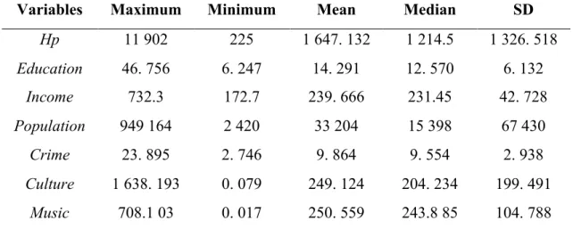
Table 2 presents the descriptive statistics for all the variables tested. As mentioned before, the house prices are expressed in thousands of Swedish Krona. During the period examined one can observe that there is a large difference between the mean value of house prices compared to the maximum. Further, education is a variable the has a large difference between its maximum value 46. 756 and its minimum 14.291, which is interesting as the education policies in Sweden should make the share of people with higher education more equally distributed. The mean annual income does not show much fluctuations, as it ranges from the values 172.7 and 732.3 and has a mean value of 239.666. However, for the independent variable population there is a large difference between the maximum and the minimum values at 949 164 and 2 420 respectively. Crime is a variable that has very little fluctuations, as the maximum value at 23.895 is not much larger than the minimum value at 2.746. In addition, the mean value at 9.864 is not far
from either maximum or minimum compared to the other variables which show bigger fluctuations. The fluctuations in the variable music are not as big as the fluctuations in the variable culture. The mean values for the two variables are rather equal, with music and culture have the mean values of 250.559 and 249.124 respectively. However, the maximum values are not as close to each other as the spending on culture has a maximum value that is two times higher than the maximum value for how much each municipality spend on music per capita. Further, for both of the variables the minimum values are very low and close to each other, again showing that the variable culture has larger fluctuations compared to the variable music.
Table 2. Descriptive statistics
Variables Maximum Minimum Mean Median SD
Hp 11 902 225 1 647. 132 1 214.5 1 326. 518 Education 46. 756 6. 247 14. 291 12. 570 6. 132 Income 732.3 172.7 239. 666 231.45 42. 728 Population 949 164 2 420 33 204 15 398 67 430 Crime 23. 895 2. 746 9. 864 9. 554 2. 938 Culture 1 638. 193 0. 079 249. 124 204. 234 199. 491 Music 708.1 03 0. 017 250. 559 243.8 85 104. 788 3.1.3 Correlation analysis
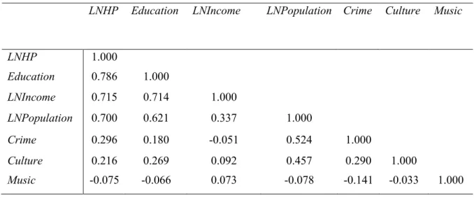
As shown in Table 3, the correlation between the variable income and education is rather high, which is predicted following the previous research on human capital. To see if the result changes, one regression will be estimated without the variable income and another without education as robustness checks. Further, the correlation between income and house prices is also high, also supported by previous research regarding the determinants for house prices. Further, there is a negative correlation between income and crime, which is also in line with the theories on human capital.
N=2900.
Variables house prices and income are expressed in thousands of Swedish Krona. Variable education is expressed in percent.
Table 3. Correlation analysis
LNHP Education LNIncome LNPopulation Crime Culture Music
LNHP 1.000 Education 0.786 1.000 LNIncome 0.715 0.714 1.000 LNPopulation 0.700 0.621 0.337 1.000 Crime 0.296 0.180 -0.051 0.524 1.000 Culture 0.216 0.269 0.092 0.457 0.290 1.000 Music -0.075 -0.066 0.073 -0.078 -0.141 -0.033 1.000 3.2 Empirical model
As this paper examines the relationship between house prices and education, the model has house price as a function of education. In addition to education, other explanatory variables that has been mentioned in previous literature to influence house prices is included in the model. The estimation model used in this paper is as follows:
𝐿𝑁𝐻𝑜𝑢𝑠𝑒 𝑝𝑟𝑖𝑐𝑒*+ = 𝛽>+ 𝛽@𝑒𝑑𝑢𝑐𝑎𝑡𝑖𝑜𝑛*+ + 𝛽A𝑙𝑛𝑖𝑛𝑐𝑜𝑚𝑒*++ 𝛽B𝑙𝑛𝑝𝑜𝑝𝑢𝑙𝑎𝑡𝑖𝑜𝑛*++
𝛽C𝑐𝑟𝑖𝑚𝑒*++ 𝛽D𝑐𝑢𝑙𝑡𝑢𝑟𝑒*++ 𝛽E𝑚𝑢𝑠𝑖𝑐*++ 𝑢*+
where 𝐿𝑁𝐻𝑜𝑢𝑠𝑒 𝑝𝑟𝑖𝑐𝑒*+ is the house price in municipality 𝑖 at time 𝑡 in logarithm form. 𝐸𝑑𝑢𝑐𝑎𝑡𝑖𝑜𝑛*+ is the share of higher education in municipality 𝑖 at time 𝑡. 𝐿𝑛𝑖𝑛𝑐𝑜𝑚𝑒*+ and 𝑙𝑛𝑝𝑜𝑝𝑢𝑙𝑎𝑡𝑖𝑜𝑛*+ are the variables income and population, in logarithm form as they are
the only variables in this model that are not expressed as shares. The remaining variables are crime per capita, as well as culture and music spending per capita in each municipality. 𝑈*+ is the error term that capture other factors that may influence house prices that the explanatory variables used in this paper have not.
3.3 Method
Using panel data can measure effects that cannot be detected by using pure time series or cross-section data. Panel data makes it possible to study to more complicated cases as it combines both time and cross-section observations as it gives more informative data and more variability. The method used in this paper for the empirical testing is Pooled Ordinary Least Squares (OLS), estimating relationship between house prices and higher education levels, using a longitudinal dataset over the years 2008-2017. When using the method pooled OLS there may be a risk that the uniqueness of the data is missed as all
the data is lumped together. To take into account the uniqueness in this model, even though the data has been pooled, year dummies are added in one of the models estimated. As shown in the correlation table, the independent variables education and income are highly correlated, therefore having both of them in a regression will expose the results to multicollinearity. Because of this there will be four different models tested in this paper. Model (1) includes the independent variables education, population, crime, culture and music. Model (2) tests for the independent variables are income, population, crime, culture and music. Model (3) includes all the independent variables; education, income, population, crime, culture and music. As shown in the correlation table, the variable income and education are correlated, therefore the possibility of the model suffering from multicollinearity is to be taken into consideration. Finally, model (4) includes all explanatory variables excluding income. In addition, year variables are added to give an indication if the pattern changes throughout the years. The year dummies will capture the influence of time-series trends in the model. Further, the year dummies are added in order to capture aggregate trends which have been failed to be detected by the independent variables in the model.
4 Empirical result
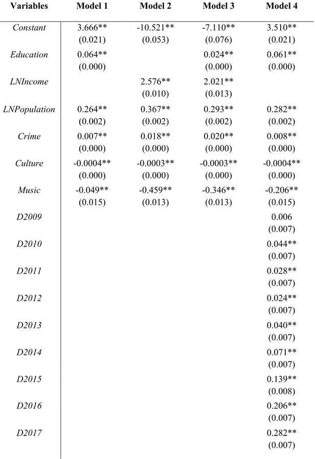
Table 4. Pooled OLS regression outputs. Dependent variable House prices in
logarithmic form.
Variables Model 1 Model 2 Model 3 Model 4
Constant 3.666** -10.521** -7.110** 3.510** (0.021) (0.053) (0.076) (0.021) Education 0.064** 0.024** 0.061** (0.000) (0.000) (0.000) LNIncome 2.576** 2.021** (0.010) (0.013) LNPopulation 0.264** 0.367** 0.293** 0.282** (0.002) (0.002) (0.002) (0.002) Crime 0.007** 0.018** 0.020** 0.008** (0.000) (0.000) (0.000) (0.000) Culture -0.0004** -0.0003** -0.0003** -0.0004** (0.000) (0.000) (0.000) (0.000) Music -0.049** -0.459** -0.346** -0.206** (0.015) (0.013) (0.013) (0.015) D2009 0.006 (0.007) D2010 0.044** (0.007) D2011 0.028** (0.007) D2012 0.024** (0.007) D2013 0.040** (0.007) D2014 0.071** (0.007) D2015 0.139** (0.008) D2016 0.206** (0.007) D2017 0.282** (0.007)
Obs. 2 900 2 900 2 900 2 900
Adj. 𝑅A 0.6953 0.7370 0.7798 0.7111
Model (1) shows that all the results are statistically significant for all independent variables at a significance level of 1%. The log-level relationship between house prices and education shows that 𝛽@ takes on the value of 0.064, indicating that one unit increase
in the coefficient will increase house prices with 6.4%. In this model the variable income is omitted as a robustness check, as its high correlation with variable education may cause multicollinearity, making it possible for wrong interpretations of the result. For the variable population, the result is interpreted differently as the relationship between that independent variable and house price is log-log. With one percent increase in population, house prices will only increase by 0.264%. The independent variable crime takes on a positive coefficient, the value for 𝛽C being 0.007 at a 1% significance. This states that a one unit increase in crime will increase house prices by 0.7%. Even though the value is low, it is still statistically significant. As for the variables culture and music, they take on negative values in the regression output. They indicate that a one unit increase in culture and music will cause a decrease in house price by 0.4% and 4.9%, respectively.
In model (2) the most visible difference is the negative coefficient for the constant, which could be interpreted as the house price being negative when all independent variables are zero, which is not likely to be possible in reality. Further, this model includes income as an independent variable, showing that one percent increase in income causes an 2.576% increase in house prices. In this model the coefficients for both the independent variables population and crime are higher than in model (1). Again, the coefficients for culture and music take on negative values in the regressions output, indicating that one unit increases in those independent variables cause decreases in house prices.
Model (3) includes all independent variables in the regression and looking at the adjusted 𝑅A values, this model appears to be the best. The value for the variable education is lower
than at the value 0.024 compared to the value in model (1) at 0.064. The same applies for the variable income in this model as the value has lowered to 2.021 compared to the values in model (2) at 2.576. For the variable population, the value in model (3) is higher than model (1), at the value 0.293. The independent variable crime takes on the highest value in model (3) at 0.020. This regression output indicates that at one unit increase in crime, house prices increase by 2% as this variable has a log-linear relationship with the dependent variable. For the remaining coefficients in model (3), they take on negative values as they have in model (1) and (2).
** Denotes significance at a 1% level. * Denotes significance at a 5% level.
Source: Statistics Sweden (2019) and Bra (2019). Source: Statistics Sweden (2019) and Bra (2019). Source: Statistics Sweden (2019) and Bra (2019).
The final model, (4), includes all independent variables except income in order to ensure that there will be no multicollinearity in the model. In addition, model (4) includes year dummies for all years in the dataset, excluding the first year. When the year dummies are added, some of the coefficients may change signs as it controls for the year effects. The results in model (4) shows that house prices have an increasing trend throughout the years, and all the results are statistically significant at 1% except for year 2009. Further, one can see that the increases becomes larger through the years, starting for year 2009 with a coefficient value of 0.006 to the final year 2017 with the coefficient value of 0.282. However, even though the year dummies are added in the model estimated, the coefficients for the education, population and crime variables continue to be positive. This shows that even though the year effects are controlled for the signs of the coefficients do not change. The same idea applies for the coefficients for the variables culture and music, as they remain negative.
5 Discussion
This paper sets out to examine if higher education levels, bachelor’s degree or above, has an increasing effect on house prices in Sweden. As shown in table 4, for the 290 municipalities in Sweden this idea holds. The idea that higher human capital acquired through education leads to higher income is not new (Eaton & Eckstein, 1997; Cooper & Luengo- Prado, 2015). However, this paper shows that not only does income have an increasing effect on house prices, but higher education does as well. Model (1) in the regression results show that education does indeed have a positive relationship with house prices. But, in contrast to the study done by Cooper and Luengo-Prado (2015), the result in this paper does not show the causality relationship between human capital and house prices. Cooper and Luengo (2015) take the standpoint in their paper that living in regions where house prices are higher, will give the residents a higher inclination to obtain higher human capital whereas this paper takes the standpoint that the causality is the other way around. Further, people living in areas with higher house prices often have higher income, driving up the house prices. This could be the way higher human capital acquired by higher education influences the house prices.
Becker (1994) states that investing in education is a wise investment done by the government as the return is high. This is also confirmed by Schultz (1961), arguing that education is a variable that should be taken into account as this improves economic growth and the overall quality of life. This is something that Sweden has done, in an effort to become a welfare-state (Schön, 2008). The fact that education in Sweden is free and has been for a while should make the argument stated by Cooper and Luegno-Prado (2015) not hold for the case of Sweden. This is because they state that children living in areas with higher house costs have families which can provide their school cost, but in Sweden all education is free. This implies that the location of your residence should not affect your ability to acquire higher human capital through education. However, as shown in the descriptive statistics in table 2 the difference between the minimum and maximum value for the variable education is quite big, meaning that the residence does seem to matter as people with higher education is clustered in one place. A different way to reason this result could be to view the cost of education the way Mincer (1958), as an opportunity cost. This is because people choosing to pursue a higher education make an active choice to forgo immediate income, which is not a possibility for all students.
Higher income leads to higher house prices, as the two variables are highly correlated. In addition to the result from the correlation analysis in table 3, the regression outputs in table 4 shows also that higher income leads to higher house prices. Model (2), where income is included and the variable education excluded, exhibit a regression result that is in line with Claussen (2013) and Asal (2018), stating that in Sweden income is an influential variable in house prices. The regression result shows that as income increases so does the house prices, making it possible to draw the conclusion that there may be outliers creating cities where the ones that have higher income push out residents with
lower income, creating the a higher cost of living as well as a higher rent premium as discussed by Gyourko et al. (2006).
Following the human capital theory, higher human capital may lead to higher quality of life as well as higher income. This could be a reason why crime and income are negatively correlated as people with higher quality of life have lower incentives to commit crime. The regression result show in table 4, where crime takes on positive sign in relation to house prices is not unique (see e.g. Lynch & Rasmussen, 2001; Tita et al., 2006). The reasoning behind it is that the areas with higher house prices have more crimes reported because they are more willing to report the crimes to authorities. This does not mean that in regions with lower house prices, fewer crimes are committed, only that the crimes are not reported to authorities. If this idea discussed by Tita et al. (2006) holds for Sweden it can lead to a skewed result in this paper, implying that higher crime rates increases house prices. The idea that higher crime rates would attract people to move to those regions, and in turn increase the demand for housing, is contradicting to the research done by Glaeser et al. (2001) and Gibbons and Machin (2008). They state that if the crime rates are lower, this will attract more people to move into those regions, increasing the demand for housing.
The previous research concerning which factors have the biggest impact, and Barot (2001) argues that population is one of the main factors for the influences in the Swedish house market. That increasing population has an increasing effect on the Swedish house markets is also confirmed by this paper as the result in table 4 shows. The inclination is that if the population increases, the demand for housing will increase at a rate that the demand cannot keep up with. However, this paper does not take into the consideration if the house prices are a result of the demand for housing or if the demand is based on the house prices that already exist in an area. This is discussed by Barot and Yang (2002), which way the causality goes. The implications are that the higher housing cost could discourage people to cluster into bigger cities, even though studies by Eaton and Eckstein (1997) shows that living in a big city might lead to higher income. Nevertheless, as the table 4 shows, the regression results show that increases in population does indeed result in increase in house prices. Blaseio and Jones (2019) and Leguizamon and Leguizamon (2017) discuss about the fact that clustering of higher human capital will lead to increasing house prices. However, the population variable in this paper is not exclusively people with higher human capital, therefore this paper cannot make the same conclusion as Blaseio and Jones (2019) and Leguizamon and Leguizamon (2017).
Scholars argue that lowering the entry barrier into a region will increase its attractiveness and thereby increase house prices. By creating more diversity, meaning not only having residents with high income and high human capital, which is defined by higher education levels, is the way to make it more attractive (Florida & Mellander, 2010). This can be done by creating more consumer amenities (Glaeser, 2001; Shapiro, 2006; Storper & Scott, 2009). This paper shows how the variables culture and music, which represent the
consumer amenities in each municipality, affects house prices. The result in table 4 shows the values contradicting previous literature, as the results in this paper shows that consumer amenities does not increase house prices. These results do not change for model (4) either, even when year effects are taken into account. Further, the high concentration of high human capital that table 2 shows with the high maximum value of variable education confirms what Florida (2002) argues about clustering of high human capital. Taking this into account, this study has proven that education has an increasing impact on house prices, which is in line with Blaseio and Jones (2019), contradicting Glaeser (2001) regarding consumer amenities making a residence attractive.
6 Conclusion
This paper examines if higher education leads to higher house prices in Sweden. Studies have shown that clustering of high human capital has a tendency to drive up the house prices in those regions, driving out people with lower income as the living costs are too high. The hypothesis for this study is as follow; higher education leads to higher human capital, people with higher human capital cluster leading to cities offering higher income and which in turn increases the living costs in cities.
The data used in this paper is secondary retrieved from Statistics Sweden and Bra in order to examine the 290 municipalities over a ten-year span between 2008-2017. The method used is Pooled OLS, and the result is divided into for different models. The main difference in the models is that the independent variables education and income are substituted in model (1) and (2) as they are highly correlated to each other. This is done as a robustness check in order to isolate the model from problems with multicollinearity. Model (3) includes both variables as well as population, crime, culture and music. As shown in table 4 the regression results do not change drastically from the previous models tested. The final model, (4), includes all independent variables excluding income but adds year dummies. This in included to make sure that the previous models results have not been affected by aggregate trends that have failed to be detected by the independent variables. Throughout the models tested in this paper, the explanatory variable education shows an increasing effect in house price. The same applies for the explanatory variable income, which is in line with previous research.
Education in Sweden is free and has been for a long time due to the policy changes made in the first half of the Second World War. This policy should have made the inequality lower between the different municipalities, as the location of living should not have affected the ability to acquire higher human capital. However, as shown in the descriptive statistics in table 2, the share of people with higher education is rather unequal between the municipalities as the gap between the maximum value of 46. 756% and the minimum value of 6. 247% is big.
Consumer amenities provided in some regions should according to theory make it more desirable to move there, increasing the demand for housing in those regions. However, this paper comes to the conclusion that consumer amenities are not the driving forces for higher house prices in Swedish municipalities as the variables culture and music, which are the estimators used to test for consumer amities are negatively related to the house prices.
In conclusion, this paper has only shown that higher education has a positive relationship with house prices house prices. Education is not the only factor influencing, nor has this paper proven that it is the most prominent determinant for house prices. As education and income are highly correlated, the result is not surprising. The reason why education has a
positive relationship with house prices could be due to the fact that people with higher human capital move to cities which offer higher wages, a positive agglomeration effect. This could be high enough to outweigh the negative agglomeration effects such as the high living cost in a clustered city.
6.1 Future research
For future research, more factors that influence house prices could be included in the model. Moreover, dummies could be included to divide the municipalities in larger areas and test if the natural amenities have an effect on the housing prices. If crime is to be used in future research as an explanatory variable, the different types of crime could be divided as this may lead to different results instead of summarizing all types of crimes into one variable as done in this paper.
References
Barot, B. (2001). An Econometric Demand-Supply Model for Swedish Private Housing.
European Journal of Housing Policy 1(3), pp. 417-444.
Barot, B. & Yang, Z. (2002). House Prices and Housing Investment in Sweden and the UK: Econometric Analysis for the Period 1970-1998. Review of Urban and Regional
Development Studies 14(2), pp. 189-216.
Becker, G. (1994). Human capital (3rd ed.). Chicago: The University of Chicago Press. Blaseio, B. & Jones, C. (2019). Regional Economic Divergence and House Prices: A Comparison of Germany and the UK. International Journal of Housing Markets and
Analysis.
Bowles, S. & Gintis, H. (1975). The Problem with Human Capital Theory—A Marxian Critique. The American Economic Review 65 (2), pp 74-82.
Brottsforebyggande Radet. (2019). About Bra. Retrieved March 3, 2019 from https://www.bra.se/bra-in-english/home/about-bra
Brottsforebyggande Radet. (2019). Gör Din Egen Sokning. Retrieved 14 August 2019, from http://statistik.bra.se/solwebb/action/anmalda/urval/sok
Claussen, C. (2013). Are Swedish Houses Overpriced?. International Journal of Housing
Markets and Analysis 6(2), pp. 180-196.
Cooper, D. & Luengo-Prado, M. (2015). House Price Growth When Children Are Teenagers: A Path to Higher Earnings?. Journal of Urban Economics 86(1), pp 54-72. Duranton, G. & Puga, D. (2003). Micro-foundations of urban agglomeration economics. In J. Henderson & J. Thisse, Handbook of Regional and Urban Economics (4th ed.), pp
2061-2117.
Eaton, J. & Eckstein, Z. (1997). Cities and growth: Theory and evidence from France and Japan. Regional Science and Urban Economics 27, pp 443-474.
Florida, R. (2002). The Economic Geography of Talent. Annals of the Association of
American Geographers, 92 (4), 743-755.
Florida, R. & Mellander, C. (2010). There Goes the Metro: How and Why Bohemians, Artists and Gays Affect Regional Housing Values. Journal of Economic Geography
Gibbons, S. & Machin, S. (2008). Valuing School Quality, Better Transport, and Lower Crime: Evidence From House Prices. Oxford Review of Economic Policy 24(1), pp. 99-119.
Glaeser, E. (2011). Triumph of the city. New York: Penguin Books.
Glaeser, E. & Gottelieb, J. (2009). The Wealth of Cities: Agglomeration Ecnomies and Spatial Equilibrium in the United States. Journal of Economic Literature 47 (4), pp 982-1028.
Glaeser, E., Kolko, J. & Saiz, A. (2001). Consumer City. Journal of Economic Geography
1, pp. 27-50.
Gujarati, D. & Porter, D. (2009). Basic Econometrics (5th ed.). New York: McGraw-Hill
Education.
Gyourko, J., Mayer, C. & Sinai, T. (2006). Superstar Cities. NBER Working Paper (12355) National Bureau of Economic Research.
Henrekson, M., Jonung, L. & Stymne, J. (1996). Economic growth and the Swedish model. In: N. Crafts and G. Toniolo, ed., Economic Growth in Europe since 1945, 1st ed. Cambridge: Cambridge University press, p.240-289.
Hort, K. (1998). Determinants of Urban House Price Fluctuations in Sweden 1968-1994.
Journal of Housing Economics 7(1), pp. 93-120.
Leguizamon, J.S. & Leguizamon, S. (2017). Disentangling the Effect of Tolerance on Housing Values: How Levels of Human Capital and Race Alter the Link Within the Metropolitan Area. The Annals of Regional Science 59(2), pp 371-392.
Lynch, A., & Rasmussen, D. (2001). Measuring the impact of crime on house prices. Applied Economics, 33(15), pp. 1981-1989.
Lyons, R.C. (2012). The Real Value of House Prices: What the Cost of Accommodation Can Tell People. Journal of the Statistical and Social Inquiry Society of Ireland 41(1), pp 71-91.
Magnusson, L. (2000). An economic history of Sweden. (8 edition). Chicago: Harvard 1. Mincer, J. (1958). Investment in Human Capital and Personal Income Distribution.
Myndigheten för Kultur Analys. (2019). Samhällets Utgifter för Kultur. Retrieved 11 April 2019, from https://kulturanalys.se/statistik/samhallets-kulturutgifter/
Oecd.org. (2019). Better Life Index. Retrieved February 10, 2019 from http://www.oecdbetterlifeindex.org/countries/sweden/
Schön, L. (2008). Sweden – Economic Growth and Structural Change, 1800-2000. Retrieved January 02, 2019, from Lund University. Retirved from: http://eh.net/encyclopedia/sweden-economic-growth-and-structural-change-1800-2000/
Schultz, T. (1961). Investment in Human Capital. The American Economic Review 51 (1) American Economic Association, pp. 1-17.
Shapiro, J. (2006) Smart Cities. The Review of Economics and Statistics 88 (2) The MIT Press, pp. 324-335.
Spence, M. (1973). Job market signaling. Quarterly Journal of Economics, 87(3), pp. 355-374.
Storper, M. & Scott, A. (2009). Rethinking human capital, creativity and urban growth.
Journal of Economic Geography 9(2), pp. 147-167.
Sweetland, S. (1996). Human Capital Theory: Foundations of a Field of Inquiry. Review
of Educational Research 66 (3) American Educational Research Association, pp.
341-359.
Tan, E. (2014). Human Capital Theory: A Holistic Criticism. Review of Educational
Research 84(3), pp. 411-445.
Tita, G., Petras, T., & Greenbaum, R. (2006). Crime and Residential Choice: A Neighborhood Level Analysis of the Impact of Crime on Housing Prices. Journal of
Quantitative Criminology, 22(4), pp. 299-317.
Wu, J. & Gopinath, M. (2008). What Causes Spatial Variations in Economic Development in the United States? American Journal of Agricultural Economics 90 (2), pp. 392-408.