Green Bond’s co-movement with the treasury bond, corporate bond, stock, and carbon markets during an economic recession

(1)

Green Bond’s co-movement with the

treasury bond, corporate bond,

stock, and carbon

markets during an economic

recession

MASTER DEGREE PROJECT

THESIS WITHIN: Business Administration NUMBER OF CREDITS: 15

PROGRAMME OF STUDY: International Financial Analysis AUTHORS: Isac Lago, Niousha Karimi

TUTOR:Haoyong Zhou

(2)

I

Master Thesis Project in Business Administration

Title: Green Bond’s co-movement with the treasury bond, corporate bond, stock, and carbon markets during an economic recession

Authors: Isac Lago and Niousha Karimi Tutor: Haoyong Zhou

Date: 2021-05-24

Key terms: Green Bonds, Conventional Bond Market, Stock Market, Carbon Market, Co-movement, DCC-GARCH, Economic Crisis

Abstract

Background: With the tremendous growth of the Green Bond (GB) market, understanding the relationship of the GB market with other financial markets gains importance. The Covid-19 pandemic causing a recession in most major economies creates an opportunity to see the co-movements of the GB market with other financial markets under a period of economic crisis. Purpose: This study aims to use the economic contraction catalyzed by the 2020’s Covid-19 pandemic as a means to investigate the co-movements between the GB and the treasury bond, corporate bond, stock, and carbon markets during an economic recession. Through this, we intend to find if co-movements of the GB market have changed, and if so, how.

Method: As the collected data is time-series data, Augmented Dickey-Fuller and Ljung-Box tests are utilized for preliminary testing. Thereafter, a univariate-GARCH model is used for volatility modeling. Moreover, the DCC-GARCH model has been conducted to determine the co-movements between the markets.

Conclusion: The results of the study show that in the case of GB, treasury, and corporate bond markets, no considerable changes were observed in the co-movement among the two different sample periods. Moving to the stock and GB markets, it was found that the co-movement increased at the beginning of the crisis. However, for the whole crisis period, no substantial changes can be seen in comparison to the pre-crisis period. Furthermore, the co-movement between the two markets was found to be weak in general. Moving on to the results obtained for GB and carbon markets, at the start of the crisis, a sharp fall can be observed. When compared to the pre-crisis period, the co-movement showed a slight increase, yet very weak. Furthermore, it was observed that the co-movement between the two markets has been weak during the whole sample period.

(3)

II

Acknowledgments

We would like to express our gratitude to the people who have supported and encouraged us during the process of writing this thesis. Firstly, we would like to express our sincere gratitude to Toni Duras for his help with the methodology. We would also want to thank Haoyong Zhou for his supervision. Lastly, we would like to thank the opposing team in the thesis seminars for providing us with insightful feedback.

(4)

III

3.1 Scientific Methodology ... 18 3.1.1 Research philosophy... 18 3.1.2 Research approach ... 19 3.1.3 Research design ... 19 3.1.4 Literature search... 20 3.1.5 Research quality ... 21 3.2 Data ... 22 3.2.1 Market representatives ... 22 3.2.2 Time period ... 29 3.3 Method of analysis ... 30 3.3.1 Preliminary tests... 30 3.3.2 Modeling volatility... 31 3.3.3 Capturing co-movements ... 34

4. Analysis and results ... 36

4.1. Returns ... 36

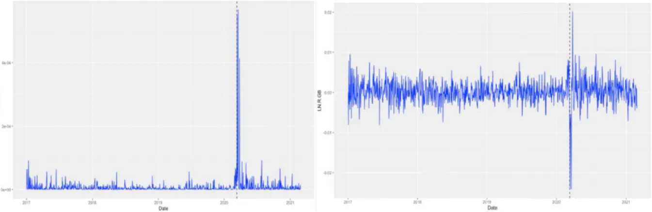
4.1.1 Green bond market ... 36

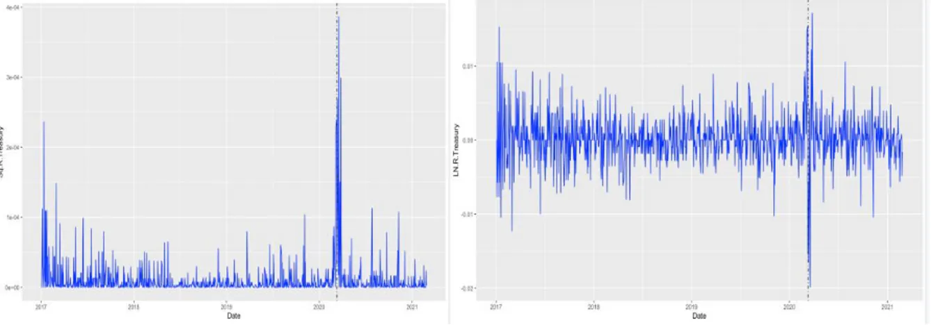
4.1.2 Treasury bond market ... 37

4.1.3 Corporate bond market ... 38

4.1.4 Stock market ... 38

4.1.5 Carbon market ... 39

4.2 Descriptive statistics ... 40

4.2.1 Correlation analysis ... 41

(5)

IV

4.3.1 Augmented Dickey-Fuller test ... 42

4.3.2 Ljung-Box test, ACF and PACF ... 43

4.4 Modelling volatility ... 45

4.5 DCC-GARCH model ... 52

4.7 Discussion ... 56

4.7.1 GB and CB markets ... 56

4.7.2 GB and stock markets ... 57

4.7.3 GB and carbon markets ... 58

5. Conclusions ... 60

6. Implications ... 62

6.1 Theoretical contributions ... 62

6.2 Practical contribution ... 63

6.3 Limitations ... 63

6.4 Areas of future research ... 64

References ... 66

Appendices ... 72

Appendix A: Correlation tables ... 72

Appendix B: Augmented Dickey-Fuller (ADF) test outputs... 74

ADF for S&P Green Bond Index... 74

ADF for State Street Global Treasury Bond Index Fund ... 75

ADF for iShares Global Corp Bond UCITS ETF ... 76

ADF for MSCI World ... 77

ADF for EEX-EUA Co2 Emissions ... 78

Appendix C: Q-statistic and p-values of Ljung-Box test ... 79

(6)

V

List of Figures

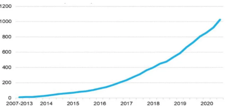
FIGURE 1.CUMULATIVE GREEN BOND ISSUANCE BY QUARTER (2007Q3-2020) ...3

FIGURE 2.RESEARCH ONTOLOGY ... 18

FIGURE 3.RESEARCH PROCESS ... 19

FIGURE 4. ISHARES GLOBAL CORPORATE BOND ... 24

FIGURE 5.RETURNS OF S&PGREEN BOND INDEX... 36

FIGURE 6.RETURNS OF STATE STREET GLOBAL TREASURY BOND INDEX FUND ... 37

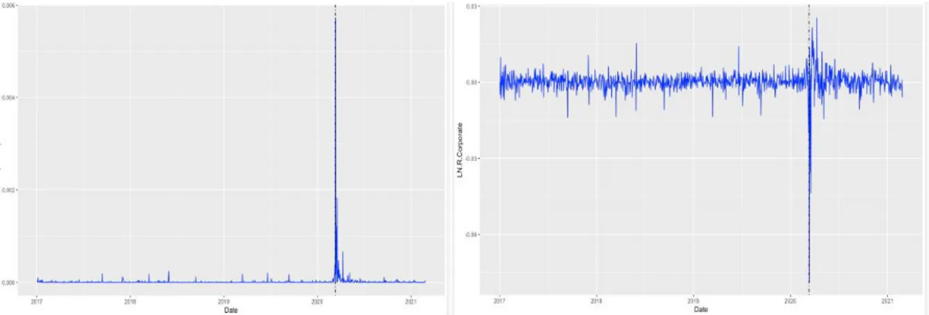
FIGURE 7.RETURNS OF ISHARES GLOBAL CORPORATE BOND UCITSETF ... 38

FIGURE 8.RETURNS OF MSCIWORLD ... 38

FIGURE 9.RETURNS OF EEX-EUACO2EMISSIONS ... 39

FIGURE 10.ACF AND PACF ... 44

FIGURE 11.CONDITIONAL STANDARD DEVIATION ... 51

FIGURE 12.DYNAMIC CONDITIONAL CORRELATION ... 55

List of Tables

TABLE 1.SUMMARY OF THEORETICAL FRAMEWORK ... 17

TABLE 2.RETURNS FOR ISHARES GLOBAL CORPORATE BOND ... 25

TABLE 3.GEOGRAPHICAL DISTRIBUTION OF ISHARES GLOBAL CORPORATE BOND UCITSETF ... 25

TABLE 4.PERFORMANCE OF STATE STREET GLOBAL TREASURY BOND INDEX ... 26

TABLE 5.GEOGRAPHICAL EXPOSURE OF STATE STREET GLOBAL TREASURY BOND INDEX ... 26

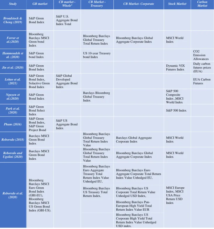
TABLE 6.PREVIOUS LITERATURE MARKET PROXIES ... 28

TABLE 7.DESCRIPTIVE STATISTICS OF LOG RETURNS ... 40

TABLE 8.CORRELATION ANALYSIS ... 41

TABLE 9.ADF TEST ... 42

TABLE 10.ARMA(0,0)-ARCH(3) RESULTS... 47

TABLE 11.ARMA(1,0)-ARCH(3) RESULTS... 47

TABLE 12.ARMA(0,0)-GARCH(1,1) RESULTS ... 48

TABLE 13.ARMA(1,0),GARCH(1,1) RESULTS... 48

TABLE 14.LJUNG-BOX TEST ON RESIDUALS WEIGHTED STANDARDIZED ... 49

(7)

1

Abbreviations

ACF: Autocorrelation Function ADF: Augmented Dickey-Fuller

ARMA: Autoregressive Moving Average

ARCH: Autoregressive Conditional Heteroskedasticity CBs: Conventional Bonds

DCC: Dynamic Conditional Correlation EEX: European Energy Exchange ETF: Exchange Traded Fund EUA: European Union Allowance

GARCH: Generalized Autoregressive Conditional Heteroskedasticity GBs: Green Bonds

GFC: Global Financial Crisis NAV: Net Asset Value

PACF: Partial Autocorrelation Function TER: Total Expense Ratio

(8)

2

1. Introduction

_____________________________________________________________________________________________

This chapter familiarizes the reader with green bonds and provides a general overview of the topic researched in this thesis. Moreover, an explanation of the identified problem is provided. The last part of this chapter focuses on clarifying the research purpose as well as the research question.

1.1 Background

Sustainable development is gaining more importance in today's world. When talking about sustainability, environmental protection and climate awareness are among the main concerns. Phenomena such as climate change, which is mainly due to greenhouse gas emissions created by human activities, have affected the environment in various ways (NASA Global Climate Change, 2021). As the issue calls for well-thought and deliberate actions, in recent years more attention has been brought to environmental topics. An example is the Paris Agreement, adopted in December 2015 by 196 parties, which is an international legal bind on climate change with the purpose of limiting global warming, with an ultimate goal of reaching a climate-neutral world. Through the nationally determined contributions (NDCs), participant countries are required to communicate their action plans regarding reducing green gas emissions (United Nations Framework Convention on Climate Change [UNFCCC], n.d.).

Together with this movement towards sustainable development, remarkable growth in sustainable finance is seen. Sustainable finance is when investors consider social, environmental, and governance factors in their investment decisions, leading them to make long-term investments in activities and projects that are targeted towards sustainability (Boffo & Patalano, 2020). Global Sustainable Investment Alliance (GSI Alliance, 2018) has indicated in their 2018 report that sustainable investments in the five1_{major markets have reached USD 30.7 trillion, showing a 34} percent increase in comparison to 2016. A concept that has been developed due to the increased demand for sustainable investments and the growing importance of climate concerns is Green Bonds (henceforth GBs). GBs were developed by Skandinaviska Enskilda Banken (SEB), a Swedish bank, and The World Bank in 2007/2008 (SEB Group, n.d.; The World Bank, n.d.). The GB market allows investors to perform conscious investments financing climate-related projects

(9)

3

while still receiving the benefits of conventional fixed-income markets (SEB Group, n.d.). As it can be seen in Figure 1, the market has been growing progressively, reaching the milestone of cumulative issuance of USD 1 trillion in early December of 2020 (Jones, 2020; BloombergNEF, 2020). In 2020, 17 nations issued GBs to an aggregate value of 71.5 million and it is predicted that 14 additional countries will begin issuing GBs in 2021 (Jones, 2020). As new countries consider the issuance of GBs and more serious actions, such as the Paris Agreement, are being taken towards reducing negative environmental impacts, it is expected that the GB market will continue to grow.

Figure 1.Cumulative green bond issuance by quarter (2007 Q3 -2020)

Source: BloombergNEF (2020)

The remarkable growth of the GB market has motivated the authors to investigate the topic further. When investigating topics related to financial markets, a particularly important aspect is the co-movement between the markets, which can reveal important information for issuers, policymakers, as well as investors. Hence, determining the co-movements of the GBs market with other key financial markets is a crucial topic to examine.

1.2 Problem

When looking at the research on the relationship and connectedness of the GB market with other financial markets, the studies mainly look into the conventional bonds, henceforth CBs, market (Broadstock and Cheng, 2019; Ferrer et al., 2021; Nguyen et al., 2020; Pham, 2016; Reboredo & Ugolini, 2020; Reboredo et al., 2020; Reboredo, 2018) stock market (Ferrer et al., 2021; Jin et al., 2020; Park et al., 2020; Nguyen et al., 2020; Reboredo & Ugolini, 2020; Reboredo et al., 2020; Reboredo, 2018), as well as energy (Hammoudeh et al., 2020; Jin et al., 2020; Leitao et al., 2021; Liu et al., 2021; Nguyen et al., 2020; Reboredo & Ugolini, 2020; Reboredo et al., 2020; Reboredo,

(10)

4

2018), commodity market (Jin et al.,2020; Lee et al., 2020; Nguyen et al., 2020; Reboredo, 2018) and carbon (Hammoudeh et al., 2020; Jin et al., 2020; Leitao et al., 2021).

Even though the previously mentioned studies have been able to provide some insight on co-movements among GBs and some key financial markets, the literature investigating the GB market is still limited (Hachenberg & Schiereck, 2018), specifically when it comes to the period of economic recession. The study by Nguyen et al. (2020) is among the only studies investigating the co-movements of GBs with CBs, stocks, clean energy, and commodities during a world economic recession by including data from the 2007-2009 global financial crisis (GFC). At the time of the GFC, the GB market was only a fraction in size of what it is today. This can be seen by comparing the USD 0.9 billion issued in 2009 with the USD 223 billion that had been issued during 2020 as of 13th_{of December that year (Jones, 2020). Due to the GB market being relatively small during} the time of GFC, it was more likely to be influenced by the development of other markets (Nguyen et al., 2020). Furthermore, studies have shown that the co-movement changed during the market expansion of 2013 (Broadstock & Cheng, 2019; Nguyen et al., 2020; Pham, 2016). A year in which the issuance of GBs reached USD 11 billion, a 550% increase when compared to the USD 2 billion issued in 2012 (Kidney, 2014).

Considering the growth of the GB market, the results of Nguyen et al. (2020) found for the small GB market does not have to apply to the matured GB market. Hence, a study on the co-movement of the GB market with other markets under the 2020’s recession caused by Covid-19 (The World Bank, 2020a) would provide a more accurate understanding of the GB market’s co-movement with other markets in times of economic crisis. It is expected that this study will add to the existing literature, as the literature investigating the GB market is still limited (Hachenberg & Schiereck, 2018). Besides, a vast number of the current research on the topic is from the period of 2018-2021, showing that at the time the current study is being conducted (2021), the topic is still very new and offers potential. Furthermore, the increased knowledge within the GB market provided in this research can be used by GB issuers, as well as policy makers and investors. Finally, as GBs are financial instruments focused on environmental projects, research on this topic is a positive step towards reaching sustainable development.

(11)

5

1.3 Purpose

This study aims to use the economic contraction catalyzed by the 2020’s Covid-19 pandemic as a means to investigate the co-movements between the GB and other financial markets during an economic recession. Through this, we intend to find if the co-movements of the GB market have changed, and if so, how. Hence, this study is divided into the two periods of pre and during crisis. The markets included in this study are the treasury bond market, corporate bond market, stock market, and the Carbon (Co2) emission rights market, henceforth carbon market. With GBs having fixed-income markets’ fiduciary elements and the CB market being one of the largest financial markets, it would be of high interest to see how the two markets co-move during a period of recession. Since the CB market consists of a variety of different bonds, including treasuries, corporates, government-backed, and super-nationals, we have chosen to focus on the two largest parts of the CB market, namely the corporate and treasury bonds. Moving on to the stock market, the Covid-19 pandemic has caused high volatility and steep falls among global stock market indices (Statista Research Department, 2020). Hence, looking at co-movements of GB and the stock market under the period of recession can create crucial knowledge within the field. The GB and carbon markets’ prices both being affected by green policies (European Commission, 2021) and regulatory changes (European Commission, n.d.) makes it interesting to investigate the relationship between the two markets. Furthermore, only a few studies look specifically into the relationship between GB and carbon emission rights markets (Hammoudeh et al., 2020; Jin et al., 2020; Leitao et al., 2021), which creates a chance for this study to contribute to the literature on the field. Altogether, we hope to find robust results which conclude how a mature GB market co-moves with other markets during times of economic recession. As the Covid-19 pandemic has affected the global economy and most major economies have suffered from the crisis (Szmigiera, 2021), the focus of this study will be on the global markets rather than a specific geographical region.

1.4 Research question

What are the differences in the co-movements between the GB market and the treasury bond, corporate bond, stock, and carbon markets pre and during the Covid-19 crisis period?

(12)

6

2. Theoretical Framework

_____________________________________________________________________________________________

The theoretical framework presents the state of the current literature in the field and presents the reader with a deepened knowledge of the relationship between the green bond market with conventional bonds, stock, and carbon markets. The focus is on the co-movements, connectedness, and spillover effects between the assets. Furthermore, the chapter provides an overview of co-movements during the crisis period.

______________________________________________________________________________

2.1 Co-movement, connectedness, and spillover effects between GB and CB markets

Applying a DCC-GARCH model using data almost stretching as far back as the intercept of the GB market, Broadstock and Cheng (2019) examine the co-movement of GBs and CBs during the period November 2008 to July 2018. In their study, they find a shift in the conditional correlation, which measures the co-movement, during mid-2013. From the beginning of their time period until the shift, the conditional correlation is about -.04, whereas it has a value of about 0.7 post the shift until the end of their time period. Broadstock and Cheng (2019) believe this shift is a cause of the vast GB market expansion in 2013. Using DCC-GARCH for the time period November 2008 to July 2018, Pham (2016) also investigates the co-movement of the GB and CB market. Similar to Broadstock & Cheng (2019), Pham (2016) finds that the co-movement is negative from the beginning of the study’s time period until around mid-2013, after which it stays strong until the end of her time period. Using copula functions, for the time period October 2014 to August 2017, Reboredo (2018) investigates the co-movement of the GB and CB market. However, in contrast to Broadstock and Cheng (2019), as well as Pham (2016), which investigate the aggregate CB market, Reboredo (2018) looks at the individual co-movements of the treasury and corporate bond markets share with the GB market. In the study, he finds that treasury as well as corporate bonds strongly co-move with the GB market during both periods of normal price movements as well as during the tails of the distributions.

While the previous paragraph focused on the co-movement of the GB and CB market, this paragraph will be focusing on findings of the spillover effects between the GB and CB market. Reboredo’s (2018) results indicate that the GB prices are substantially affected by spillovers from

(13)

7

the treasury and corporate bond markets. Pham (2016) also investigates spillover effects between the CB and GB market. However, while Reboredo (2018) only investigated how the CB market can spill over to the GB market, Pham (2016) investigates the spillovers in both directions. The results show that shocks in the GB or CB market can cause spillover effects to the other market. Reboredo and Ugolini (2020) use a structural vector autoregressive model to investigate the price connectedness between GB and other markets. In the study, they find that the GB market is strongly affected by spillovers from corporate and treasury bonds. While the largest spillovers are found from the treasury market to the GB market, the reverse oscillations are negligible. The price spillovers are considerable in both directions between GBs and corporate bonds, a relation in which GBs are net receivers. The results show that shocks in the GB or CB market can cause spillover effects to the other market. Moreover, the spillover effects become more frequent for later observation in the time series used (Reboredo & Ugolini, 2020). Hammoudeh et al. (2020) investigates if treasuries affect the GB market prices. Specifically, they are using a time-varying Granger causality test to see if the US 10-Y treasury bills are affecting the US GB market prices during the time period 30 July 2014 to 10 February 2020. In the study, they found that from the end of 2016 to February 2020, the US 10-Y treasury bond has explanatory power for US GB market prices.

In this paragraph, the literature investigating GB and CB’s price relationships over different time horizons will be presented. Using the methodology of Křehlík and Baruník (2017). on data during October 2014 to 2019, Ferrer et al. (2021) find that the connectedness of GBs and investment-grade corporate bonds, as well as treasury bonds, are most prominent during a shorter time horizon. Specifically, a shock in the treasury or investment-grade market is usually incorporated in the GB market, or vice versa, within 5 days. They also find a strong connectedness in return and volatility between GBs and these CB markets. Based on this, they conclude that GB does not seem as a unique asset class, but it mirrors that of the treasury and investment grade corporate bond markets. Applying a rolling-window wavelet correlation framework on data within the time period November 2008 to July 2018, Nguyen et al. (2020) examine the conditional correlation of the GB and CB market over 4 different time horizons, represented by D1 to D4. D1 is used for 2-4 days, D2 for 4-8 days, D3 for 8-16 days and finally D4 represents 16-32 days. Where D1-D3 is considered as the short-run perspective and D4 as the long-run. For all time scales, they found a

(14)

8

shift in 2013, which is similar to the findings of Broadstock and Cheng (2019). Post the shift, the correlation is about 0.8, which is close to the conditional correlation found by Broadstock and Cheng (2019). However, the correlation during 2008 up until the shift is positive around 0.45, which substantially deviates from the -0.4 reported by Broadstock and Cheng’s (2019). Reboredo et al. (2020) investigate the network connectedness between GBs and different assets during different time horizons in EU and US markets during the time period October 2014 to December 2018. The study consists of different asset classes including investment-grade corporate bonds, high-yield corporate bonds, and treasury bonds. Using wavelet coherence, Reboredo et al. (2020) find that, in the EU markets, GBs strongly co-move with the treasury as well as investment-grade corporate and high-yield corporate bonds in the medium and long- term from early 2015 to late 2016. While the co-movement diminishes for the high-yield corporate bonds in late 2016, it stays strong for the investment-grade and treasury bonds until the end of the time period in 2018. For the US markets, the GB strongly co-move in the medium-term with the treasury and corporate bond markets from the beginning of 2015 to the end of their time period in 2018. The high-yield bonds have a strong and significant medium and long-term co-movement during 2015 and 2016, which then drops for the remaining time period. After investigating the co-movement of the markets, Reboredo et al. (2020) use a multivariate autoregressive model of decomposed compositions to analyze the market spillovers. The results from this process indicate that treasury and corporate bonds in the short run together explain 24% and 28% of the volatility in the EU and US markets respectively. In the long run, these numbers are 18% and 24% respectively. The price oscillations from the GB market to the corporate and treasury markets are negligible in the short and long term.

To summarize, the previous literature has found that the co-movement of the GB and aggregate CB market has remained strong since its substantial increase in mid-2013 (Broadstock & Cheng, 2019; Nguyen et al., 2020; Pham, 2016). When the co-movement of the GB market has been investigated with the treasury and corporate bond markets separately, it has been found that the co-movement of GBs and these two segments of the CB market are strong (Reboredo, 2018). When the co-movement has been analyzed during different time horizons, Reboredo et al. (2020) found that in the EU market GBs strongly co-move in the medium-term with investment-grade corporate bonds as well as treasury bonds from 2015 to 2018. For the same region, the co-movement of GBs

(15)

9

and high-yield corporate bonds was strong from 2015 to 2016. For the US markets, the GB strongly co-move in the medium-term with the treasury and corporate bond markets from the beginning of 2015 to 2018 (Reboredo et al., 2020). Literature investigating spillover effects has found that the treasury bond market transmits substantial volatility spillovers to the GB market (Hammoudeh et al., 2020; Reboredo & Ugolini, 2020; Reboredo, 2018), whereas the transmissions in the opposite directions are negligible (Reboredo & Ugolini, 2020). The previous literature has also found that that corporate bond transmits substantial spillovers (Reboredo, 2018). Similar literature has found that the spillovers are considerable in both directions (Pham, 2016; Reboredo & Ugolini, 2020). Ferrer et al. (2020) found that the connectedness of GBs and investment-grade corporate bonds, as well as treasury bonds, are so strong that it seems as GB prices mirror the prices of these markets. The previous literature has been using data including observations up until 2018(Broadstock & Cheng, 2019, Nguyen et a., 2020; Reboredo et al., 2020), 2019 (Ferrer et al., 2021; Reboredo & Ugolini, 2020), and 2020 (Hammoudeh et al., 2020).

2.2 Co-movement, connectedness, and spillover effects between GB and stock markets Various studies look at the co-movements, dependence structure, and spillover effects between GB and stock markets (Ferrer et al., 2021; Jin et al., 2020; Park et al., 2020; Nguyen et al., 2020; Reboredo & Ugolini, 2020; Reboredo et al., 2020; Reboredo, 2018). In this section of the literature review, the focus will be on the studies investigating the relationship between the GB and stock market in regard to the two markets’ co-movements, time-varying dependence, as well as spillover effects.

The study by Reboredo (2018) evaluates the dependence structure between the GB and stock market by using copula functions during the sample period of October 2014 to August 2017. After running a Pearson correlation, low coefficients have been observed between GBs and the stock market. The results from conducting copula tests, including Student-t, Gaussian, SJC, Gumbel, and Rotated Gumbel models, show a weak co-movement among the prices of stock and GB market. Furthermore, the dependence between stock and GB market is found to be time-varying and a weak symmetric tail-dependence between the two markets is detected (Reboredo, 2018). In another study conducted by Jin et al. (2020), a large and significant negative correlation is seen

(16)

10

between the returns of GB market and VIX index. Jin et al. (2020) consider the time period of December 2008 to August 2018.

Using a sample period from October 2014 up to December 2018, Reboredo et al. (2020) also confirm that there is a weak co-movement between the stock and GB market through analyzing network connectedness between GB and stock markets using wavelet coherence. The focus of the study is on the US and EU GB markets, as they have had the most active GB markets in recent years. In addition, the authors find that the co-movement shows variety in intensity over the time period as well as time horizons, with the dependence being mainly focused on the medium scale time-frequency in both EU and US markets. In addition, a study conducted by Nguyen et al. (2020) also looks into the time-frequency domain through wavelet analysis within the time period of December 2008 to December 2019. The study uses 4 different scales for the time-frequency, which are represented by D1 to D4. D1 is used for 2-4 days, D2 for 4-8 days, D3 for 8-16 days and finally D4 represents 16-32 days. Where D1-D3 is considered as the short-run perspective and D4 as the long-run. According to Nguyen et al. (2020), from 2013, the correlation between GB and the stock market has been weak, with a slight increase in the 2016-2018 time period. However, the increase in the mentioned period has been negligible. The start period of the study, namely 2008-2013, has been under the influence of the GFC, and hence a significant positive correlation has been seen. The effect of the crisis on co-movements and market relationships will be discussed in more detail in section 2.4 of this literature review. Furthermore, the GB market has been relatively small during the 2008-2013 period, making it more likely to be under the influence of other markets (Nguyen et al., 2020). All in all, Nguyen et al. (2020) report a weak co-movement between the two markets, where a lower correlation can be seen in the short-term scales rather than the long-term one. Another study by Ferrer et al. (2021) conducted on the sample period of October 2014 to December 2019 aims to analyze the time-frequency connectedness between GB and other markets, including the general stock market. The findings of the study reveal a rather weak link between GB and the stock market regardless of the time period and frequency.

Looking further into the studies, Reboredo and Ugolini (2020) use structural vector autoregression (VAR) to investigate the lagged interdependence and contemporaneous causal relations between price changes in GB and other markets. The use of the VAR model has enabled the authors to

(17)

11

perform an accurate analysis of the network links between the markets, characterize multivariate dependence, and capture indirect and direct financial shocks among the markets. Similar to the previous studies, Reboredo and Ugolini (2020) also confirm that the connection between the stock and GB market is weak. Furthermore, Reboredo and Ugolini (2020) explain that GBs can be used for the purpose of minimization of downside risk and hedging the risk of portfolios containing stocks.

When looking at the spillover effects between the two markets, it can be observed that most studies explain that there are negligible price spillovers between the stock and GB market (Reboredo & Ugolini, 2020; Reboredo et al., 2020; Reboredo, 2018). Reboredo and Ugolini (2020) measure price return spillovers between markets by decomposing the forecast error variance of the structural VAR model. Through this, it is revealed what fraction of the forecast error variance of GB prices is explained by shocks in other markets within the period of October 2014 to June 2019. Reboredo and Ugolini (2020) find negligible price spillovers between the stock and GB market. Another study by Reboredo (2018) confirms that the impact of a large price swing in the stock market would be minor on the GB prices. In addition, Reboredo et al. (2020) investigate spillover effects between GBs and the stock market through a connectedness framework, which is based on the error variance decomposition of a VAR model. Through this analysis, the transmission of price shocks between the two markets is also found to be imperceptible both in the long and short term.

In a slightly different study, Park et al. (2020) examine spillovers as well as volatility dynamics between the GB and stock market. Furthermore, the authors investigate if the asymmetric volatility seen in the return dynamics of most financial products is also true for GBs. To test the volatility spillover between the two markets, DCC-GARCH and Baba-Engle-Kraft-Kroner (BEKK) models are used within the sample period of January 2010 to January 2020. The authors find that GBs show asymmetric volatility, however, GBs’ volatility exhibits a unique characteristic of sensitivity to positive shock which is not normally seen in other financial instruments. This can be due to the increasing growth of the GB market which leads the investors to have a hopeful view towards GBs and therefore have stronger reactions to minor good news, which then results in the volatility increasing. Regarding the volatility spillovers, Park et al. (2020) report that even though some

(18)

12

volatility spillovers are seen between the two markets, neither of the markets shows a significant response to a negative shock in the other market.

From the studies, it can be concluded that there is a weak co-movement between GB and the stock market (Ferrer et al., 2021; Jin et al., 2020; Nguyen et al., 2020; Reboredo & Ugolini, 2020; Reboredo et al., 2020; Reboredo, 2018). When looking at the time-frequency, Nguyen et al. (2020) state that there is a lower correlation in the short-term scales rather than the long-term one. Whereas Reboredo et al. (2020) discuss that the time-varying dependence is mainly focused on the medium scale time-frequency in the US and EU markets. In a contradicting study, Ferrer et al. (2021) state that regardless of time period and frequency, the relationship between the two markets is weak. Whereas both studies by Reboredo et al. (2020) and Reboredo (2018) confirm that the dependence between GBs and stocks is time-varying. In addition, Reboredo (2018) finds a weak symmetric tail-dependence between the two markets. When it comes to the spillover effects between GB and the stock market, it can be said that the effects are negligible (Reboredo & Ugolini, 2020; Reboredo et al., 2020; Reboredo, 2018). Even though the study by Park et al. (2020) shows some volatility spillover, it is confirmed that there are no significant responses from the GB or stock market in case of a negative shock in either of the markets. Furthermore, Park et al. (2020) explain that the return dynamics of GBs are similar to those of other assets, with the exception of sensitivity to positive shocks.

2.3 Co-movement, connectedness, and spillover effects between GB and carbon markets While some studies are looking at the relationship between energy and the GB market (Jin et al., 2020; Liu et al., 2021; Nguyen et al., 2020; Reboredo & Ugolini, 2020; Reboredo et al., 2020; Reboredo, 2018) as well as GB and commodity market (Jin et al.,2020; Lee et al., 2020; Nguyen et al., 2020; Reboredo, 2018), the number of studies that specifically focus on GB and carbon (Co2) are scarce. This section of the literature review will focus on the research on the relationship between the carbon and GB market to provide a better overview of the link between the two markets.

Jin et al. (2020) aim to investigate the market connectedness between GB and the carbon market and try to reveal what role GBs have in hedging the risk of the carbon market using

(19)

DCC-GJR-13

GARCH, DCC-T-GARCH, and DCC-APGARCH during the time period of December 2008 to August 2018. Due to the integrated structure of financial, commodity, and energy markets, the study uses five variables including green, carbon, stock, energy, and commodity markets. Through the analysis, Jin et al. (2020) find a correlation coefficient of 0.25 between the GB index returns and carbon features return. Thereupon, the asymmetric effect and directional connectedness were tested by the authors. The findings of the article by Jin et al. (2020) suggest that GB index returns and carbon features returns have the highest connectedness among the tested variables, which are especially pronounced during periods of market volatility. Furthermore, as a hedging instrument against the risk of the carbon market, GBs are found to be suitable and effective, even in times of crisis. When looking at the GBs price movement effects on Co2 emissions, Leitao et al. (2021) provide evidence of a positive and significant effect in both low and high volatility regimes. Another study in the field by Hammoudeh et al. (2020) looks at the time-varying causality relationship between prices of the Co2 emission allowances and GBs using causality algorithms with a sample period of July 2014 to February 2020. The findings of Hammoudeh et al. (2020) show that from the beginning of the sample period until the end of 2015, a significant time-varying causality from prices of the Co2 emission allowances to GBs can be found. In 2015, the highest level of allowances was reached with a drop in oil prices, resulting in high Co2 permit demands, spelling over to the GB market. When it comes to causality from GBs to Co2 Emission Allowances, no significant causality was found by Hammoudeh et al. (2020). Park et al. (2020) found that neither the stock or CB market transmits any spillovers during negative shocks.

According to Jin et al. (2020), GBs are found to be an effective hedging instrument against the risk of the carbon market. When looking at the connectedness between the GB and Carbon feature returns, a fairly high connectedness is found especially during volatile periods (Jin et al., 2020). Leitao et al. (2021) also looks at market volatility and states that the price movements of GBs have a positive and significant effect on Co2 emissions in both low and high volatility regimes. While inspecting time-varying causalities between the two markets, Hammoudeh et al. (2020) find no significant causality from GBs to Co2 emission prices, whereas a significant time-varying causality is detected from Co2 emission allowances to GBs during the period of July 2014 (beginning of study’s sample period) to end of 2015.

(20)

14

2.4 Economic crisis and markets’ co-movements

As our study will look into if the ongoing economic crisis is accompanied by a shift in the co-movement of the GB market, researching the previous literature of GB co-co-movement during previous crises and market turbulence is of particular interest. However, the literature focusing on GB co-movement during economic crises is limited. To our knowledge, Nguyen et al. (2020) is the only study conducted with the purpose of investigating co-movements during such times. While not the main purpose of the article, Le et al. 's (2021) research which includes data up until 29 June 2020 can provide some insight into how GB co-movement with other assets during the Covid-19 economic crisis. Other studies, which disclose information regarding GBs co-movements during times of high market turbulence and its downward tail distribution are also of relevance when investigating co-movements of GBs during an economic crisis. As this literature is limited as well, we will also bring up how markets in general behave during times of recession.

Nguyen et al. (2020) found that GB co-movement with conventional bonds, commodities, and clean energy reached its peak during the last GFC. Using VIX to measure market volatility, Broadstock and Cheng (2019) concluded that the conditional correlation of GBs and CBs becomes stronger during volatile time periods. Le et al. (2021) use the methods from Diebold and Yilmaz (2012) as well as Barunik et al. (2017) to examine co-movement and spillovers between GBs, fintech stocks, cryptocurrency, and the overall stock market during the time period November 2018 to end of 2019. Then, a robustness check was done in which the results were compared with the same metrics retrieved using the time period 1 January 2020 to 20 June 2020. The results indicate that general stocks, represented by MSCI US and MSCIW are net distributors of shocks whereas GBs are net receivers from November 2018 to the end of 2019. Specifically, it is shown that GBs have the lowest transmitting effects of all the assets analyzed during this period. However, during 2020, all asset transmission effects increased, meaning that the markets’ movements became more intertwined. During this time period, GBs were a net spillover transmitter to the USD market. Although the markets became more intertwined, Le et al. (2021) show that the co-movement of stocks and GBs was weak for all analyzed time periods. Furthermore, it is seen that the long-term volatility transmissions are weaker than the short-term transmissions regardless of the time period. Jin et al. (2020) which investigated the co-movement of GBs and carbon futures finds that the co-movement is especially strong during crisis times.

(21)

15

Studies investigating how co-movements in markets in general are affected by economic or financial crises can bring some insight into how GBs co-movement possibly behaves during such times. Using wavelet decompositions of return time series, Benhmad (2013) investigated co-movements and contagion of international stock markets under different time scales during the last GFC 2007-2009. The analyzed time period is from July 2005 to June 2011. The results indicate that the co-movement is stronger during times of declining market prices than during times of rising prices. Mun and Brooks (2012) investigate how volatility affected the correlation within 15 different national stock markets during the last GFC. In the study, they split their sample, from 23/02/2007 to 26/02/2010 into the four sub-samples P1:27/02/2007 to 19/05/2008, P2:20/05/2008 to 15/09/2008, P3:16/09/2008 to 19/02/2009, and P4: 20/02/2009 to 26/02/2010. The correlation is then examined using an APARCH model. Their results indicate that during P1-P3, 75 to 77 percent of the correlation is explained by the markets’ volatility, whereas this metric for P4 was 28 percent. Based on these results, they draw the conclusion that when the GFC was more severe, and volatility more persistent, the correlation became stronger. Silvennoinen and Thorp (2013) assess the dynamic co-movements between stocks, bonds, and commodity futures from May 1990 to July 2009. In their study, they find that the assets co-movement increases over time and reached its peak during the last GFC. Using STCC-GARCH and DSTCC-GARCH models, Öztek and Öcal (2017) seek to find determinants for the correlation of stocks and commodities. The two commodity groups of interest are agricultural commodities and precious metals. The results show that during the analyzed time period, 4 January 1990 to 20 December 2012, financial crises and other volatile periods are accompanied by the strongest correlations.

2.5 Summary of the theoretical framework

To conclude the previous literature’s findings regarding the spillover effects between the GB and CB market, Pham (2016), Reboredo (2018) as well as Reboredo and Ugolini (2020) indicate that the GB prices are substantially affected by spillovers from the treasury and corporate bond markets. Reboredo and Ugolini (2020) further explain that while the largest spillovers are found from the treasury market to the GB market, the reverse oscillations are negligible. The price spillovers are considerable in both directions between GBs and corporate bonds, a relation in which GBs are net receivers. Looking at the connectedness between the two markets, Ferrer et al. (2021)

(22)

16

and Reboredo et al. (2020) confirm that CB and GB markets show strong connectedness in return and volatility. When investigating the co-movement of the GB and the aggregate CB market, previous research has found that the relationship becomes stronger over time (Broadstock & Cheng, 2019; Nguyen et al., 2020; Pham, 2016). The same conclusion has been drawn when corporate and treasury bonds co-movements with the GBs have been investigated separately (Hammoudeh et al., 2020; Reboredo, 2018; Reboredo et al., 2020). Taking a look at the relationship between these two markets during volatile time periods, Broadstock and Cheng (2019) concluded that the conditional correlation of GBs and CBs becomes stronger during times of market volatility. Furthermore, Nguyen et al. (2020) found that GB co-movement with conventional bonds reached its peak during the GFC. A finding that was confirmed by Silvennoinen and Thorp (2013) in the case of stocks, bonds, and commodities.

In the case of GB and the stock markets, the spillover effects between the two markets were found to be negligible (Reboredo & Ugolini, 2020; Reboredo et al., 2020; Reboredo, 2018). Furthermore, previous studies find a weak co-movement between GB and the stock market (Ferrer et al., 2021; Jin et al., 2020; Nguyen et al., 2020; Reboredo & Ugolini, 2020; Reboredo et al., 2020; Reboredo, 2018). The studies by Reboredo et al. (2020) and Reboredo (2018) confirm that the dependence between GBs and stocks is time-varying. When looking at the time-frequency, Nguyen et al. (2020) state that there is a lower correlation in the short-term scales rather than the long-term one. Whereas Reboredo et al. (2020) discuss that the time-varying dependence is mainly focused on the medium scale time-frequency in the US and EU markets. In contrast, Ferrer et al. (2021) state that regardless of time period and frequency, the relationship between the two markets is weak. When the relationship of the two markets is evaluated during times of market volatility, Le et al. (2021) show that even though the markets’ movements became more intertwined in 2020, the co-movement of stocks and GBs was weak for all the analyzed time periods. Analyzing the international stock market, Benhmad (2013) discusses that the co-movement is stronger during times of declining market prices than during times of rising prices. Silvennoinen and Thorp (2013) as well as Mun and Brooks (2012) also confirm that when the GFC was more severe, and volatility more persistent, the correlation became stronger.

(23)

17

Summarizing the previous literature on the connectedness of Carbon and GB markets, we found that the study by Jin et al. (2020) indicates a correlation coefficient of 0.25 between the GB index returns and carbon features return. They further confirm that the connectedness is especially pronounced during periods of market volatility. Leitao et al. (2021) also looks at market volatility and states that the price movements of GBs have a positive and significant effect on Co2 emissions in both low and high volatility regimes. While inspecting time-varying causalities between the two markets, Hammoudeh et al. (2020) find no significant causality from GBs to Co2 emission prices, whereas a significant time-varying causality is detected from Co2 emission allowances to GBs during the period of July 2014 (beginning of study’s sample period) to end of 2015.

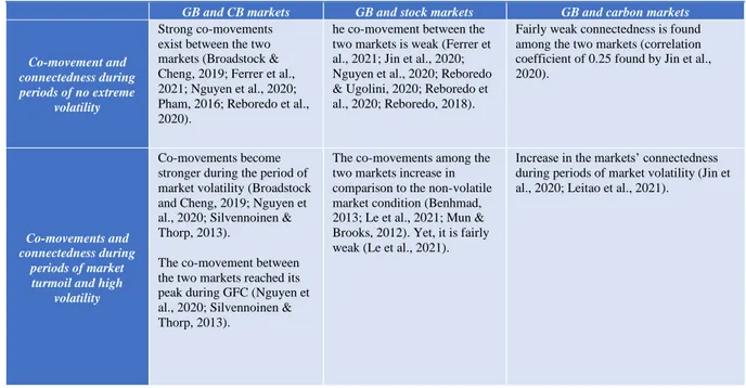
Table 1 presents a brief summary of previous literature’s overview regarding the co-movements of the markets. To make a last conclusion remark of the previous literature, as both Nguyen et al.’s (2020) and Le et al.’s (2021) results of GBs co-movements becoming greater during times of economic crises is in line with the findings of literature investigating the co-movements of other markets during these market conditions (Mun & Brooks, 2012; Öztek & Öcal, 2017; Silvennoinen & Thorp, 2013), we believe that we will find stronger co-movements during the time period capturing the covid-19 economic crisis than for the earlier subsample.

GB and CB markets GB and stock markets GB and carbon markets

Co-movement and connectedness during periods of no extreme

volatility

Strong co-movements exist between the two markets (Broadstock & Cheng, 2019; Ferrer et al., 2021; Nguyen et al., 2020; Pham, 2016; Reboredo et al., 2020).

he co-movement between the two markets is weak (Ferrer et al., 2021; Jin et al., 2020; Nguyen et al., 2020; Reboredo & Ugolini, 2020; Reboredo et al., 2020; Reboredo, 2018).

Fairly weak connectedness is found among the two markets (correlation coefficient of 0.25 found by Jin et al., 2020).

Co-movements and connectedness during

periods of market turmoil and high

volatility

Co-movements become stronger during the period of market volatility (Broadstock and Cheng, 2019; Nguyen et al., 2020; Silvennoinen & Thorp, 2013).

The co-movement between the two markets reached its peak during GFC (Nguyen et al., 2020; Silvennoinen & Thorp, 2013).

The co-movements among the two markets increase in comparison to the non-volatile market condition (Benhmad, 2013; Le et al., 2021; Mun & Brooks, 2012). Yet, it is fairly weak (Le et al., 2021).

Increase in the markets’ connectedness during periods of market volatility (Jin et al., 2020; Leitao et al., 2021).

(24)

18

3. Methodology and method

_____________________________________________________________________________________________

In this chapter, firstly, a description of the scientific methodology of the paper, including the research philosophy, approach, and design is provided. Thereupon, the literature search and research quality are discussed. In the second part of this chapter, the details regarding the data used in the study are presented. Lastly, the method of data analysis is introduced.

______________________________________________________________________________

3.1 Scientific Methodology

3.1.1 Research philosophy

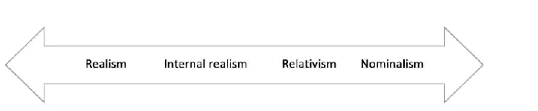
Looking at the continuum below in Figure 2, we can say that this study would be positioned on the left side, close to a realistic ontology. The reason for this is that the authors of this thesis assume that the nature of reality is external and exists independently of the observations and perceptions made about it (Easterby-Smith et al., 2018). When investigating the co-movements of the GB market with the other selected financial markets under an economic crisis, we assume that hard facts exist regarding the markets’ relationships. These facts and the science behind them can be revealed through observations that directly correspond to the topic being investigated (Easterby-Smith et al., 2018). We believe that as researchers, we are not a part of what is being observed, but rather independent from it and we view the nature of reality as external. Furthermore, we use hypothesis testing and objective methods to be able to answer the research question of the study. Thus, it would be appropriate to say that this study has a positivist epistemology, which is in line with the realistic ontology (Easterby-Smith et al., 2018).

Figure 2. Research ontology

(25)

19

3.1.2 Research approach

The current study is descriptive research, where the authors aim to obtain information on the characteristics of a particular phenomenon (Collis & Hussey, 2013). More specifically, it is aimed to reveal the co-movements of selected assets with GBs under an economic crisis. When analyzing the co-movements of GBs with other selected financial markets under an economic crisis, first, a theoretical framework of what the previous studies within the field have found was developed. Thereafter, based on the understanding of the topic provided by the previous literature as well as the literature gap, assumptions were formulated with the expectation that the co-movements would increase during the time of crisis. Further on, data was collected for each market to be able to investigate the movements. Through time series analysis, particular conclusions regarding co-movements of markets under an economic crisis were drawn. Hence, it can be said that in this paper, we move from more general interfaces to particular ones. Thus, this study has a deductive approach where first a conceptual framework is built, and then it is investigated through observations (Collis & Hussey, 2013).

Figure 3. Research process

3.1.3 Research design

As previously mentioned, hypothesis testing and objective methods are used in this paper to be able to answer the research question of the study and fulfill the purpose. Furthermore, the collected data is analyzed using statistical methods. These characteristics are in accordance with the design for quantitative research (Collis & Hussey, 2013). The quantitative research design is also in line with the realistic ontological and the positivist epistemological nature of this study, as well as the deductive research approach (Easterby-Smith et al., 2018). The main reason for using this research design is that reaching the objective of revealing the co-movements among the markets under an economic crisis would be achievable through quantitative and statistical methods. The use of qualitative methods such as case studies, grounded theory, or ethnographic research would not provide us with the proper and sufficient tools to answer the research question. As the collected

(26)

20

data in this thesis is time-series data, we conducted preliminary tests to determine the stationarity and choose an appropriate model accordingly. This type of analysis would not be feasible if a qualitative method was chosen.

3.1.4 Literature search

To conduct the literature review, the following keywords were identified: “green bond”, “co-movement”, “co“co-movement”, “spill-over effects”, spillover effects”, “correlation”, and “dependence structure”. Based on these keywords, different basic searches were conducted in the Scopus database. Firstly, the following words were searched "green bond*" and "co-movement*" or "comovement*" or "inter-relationship*" or "correlation*" or "diversification*", resulting in 15 documents. For articles related to spillover effects, the search words were “green bond*” and “tail dependence*” or “spillover effect*” or “Spill-over effect*” or “spillover*” from which 11 documents were obtained. The search was within article titles, abstracts, and keywords. No data range was chosen as the green bond market is very young and hence it was expected that the studies in the field would be mainly recent. The results from the searches were carefully inspected with regards to their relevance, and the irrelevant studies were henceforth not considered. As the literature on the GB market is still quite limited (Hachenberg & Schiereck, 2018), the references of the obtained articles were also reviewed to see if any more relevant studies could be found.

To assure that the articles used in this study are reliable, only peer-reviewed journals have been used. Besides, the 2018’s Academic Journal Guide (AJG) ranking has also been taken into consideration. The AJG ranking is a guide to the quality of the journal within the field of business and management. The ranking is from 1-4, with 4 representing the highest quality and best-executed journals. A 4* ranking represents a journal with distinction (Academic Journal Guide [AJG], 2018). This study mainly includes journals with a 2 and above ranking, meaning that the studies are of an original and acceptable standard (AJG, 2018). In the case of the Journal of Sustainable Finance and Investment with an AJG ranking of 1, the source’s normalized impact per paper (SNIP), has been checked. This is a measure of citation with a weighting based on the subject field (Massey University, 2021). The Journal of Sustainable Finance and Investment has a SNIP of 1.032 (Scopus, n.d.). A SNIP of 1 shows that the journal is cited at an average rate within the

(27)

21

journals in the same subject area (Massey University, 2021). Hence, we decided to keep the studies by Pham (2016), even though the criteria of an AJG ranking of 2 or above was not met in this case.

3.1.5 Research quality

In order to produce a study of high quality, the first aspect that has been taken into consideration is controllability. The primary condition for ensuring research controllability is that the research products, as well as the processes used to produce the outcomes, are public (Swanborn, 1996). To achieve this, the authors have clearly presented the procedures, implemented methods, as well as outcomes of all the statistical tests. Furthermore, the EViews test outputs have been provided in this thesis’s appendices. The second condition is that the products of the research should be expressed in a precise language (Swanborn, 1996). In order to fulfill this, vague expressions have been avoided when describing the outcomes. In addition, it has been taken into consideration that the results are presented in accordance with academic standards to achieve high precision. The last criterion is falsifiability. In this paper, as the research products are clearly stated and are testable, the research outcomes are falsifiable.

The next criterion for research quality is reliability. For the research to be reliable, the inter-researcher reliability needs to be legitimate, meaning that the research products should be independent of the researchers conducting the study (Swanborn, 1996). In this study, it has been ensured that the statistical tests and research processes follow a replicable and standard procedure, meaning that if any other researcher would try to reproduce the study, they would obtain the same results. In addition to being researcher independent, this study is time-independent, meaning that if the tests were conducted on the collected data at any point in time, the same outcomes would be achieved. Moreover, the products of this research are instrument independent. This means that regardless of the software and tools used to conduct the analysis, the outcomes would remain the same. Many of the tests, such as the Augmented Dickey-fuller (ADF) test have been conducted in both EViews and RStudio and the same results have been obtained. Thus, it is concluded that this research meets the reliability criteria proposed by Swanborn (1996).

Moving on to research validity, Swanborn (1996, p. 22) defines this criterion as “our propositions describe and explain the empirical world in a correct way; in a stricter sense: that they are free

(28)

22

from random as well as systematic errors”. To be able to produce research with valid outcomes, the interpretations of the research have been strictly based on the results of the statistical tests. In the case of the GARCH model, previous studies in the field have been investigated to get a clear overview of a correct interpretation of the model. When it comes to having propositions that are free of random and systematic errors, it can be hard to determine what is or is not a systematic error. Nonetheless, to minimize the chances of error, a strong foundation and understanding regarding the legitimate procedures of conduction and interpretation of the models have been attained based on the origins and the accepted standards of each model. Henceforth, these procedures have been followed as closely as possible, to ensure that the required conditions and standards are met when interpreting the results. The authors' effort has been towards describing the empirical world correctly throughout the whole research process. Thus, the validity of this study has been of high importance to the researchers, and it is expected that the outcomes are valid.

To increase the quality of the research further, we have used Microsoft Excel, EViews, and RStudio for the calculations, which has increased the objectivation of the thesis. This is in line with this study’s research philosophy, design, and approach, as we view the nature of reality as objective and external. Hence, we minimize the effect of researchers’ subjectivity. As briefly mentioned before, standardized approaches and procedures have been used in this study, which is another factor that helps with achieving better quality in the research (Swanborn, 1996). In addition, the measurements and tests have been repeated in many cases using different software to confirm no errors have been associated with conducting the tests. To ensure the transparency of the communications and the research procedures between the two authors, a research diary has been kept, in which the development of the thesis as well as any relevant notes have been constantly updated. Altogether, the paper has been constantly checked to be in line with the controllability, reliability, and validity factors.

3.2 Data

3.2.1 Market representatives

In this study, the S&P Green Bond Index was selected to measure the price movements of the GB market. State Street Global Treasury Bond Index Fund was used as a proxy for the treasury bond market and the iShares Global Corporate Bond UCITS ETF for the corporate bond market. To

(29)

23

represent the stock market, MSCI World Index was chosen. Finally, for the carbon market, EEX-EUA Co2 Emission Allowances were selected. The data for all the indices were retrieved from Thomson Reuters DataStream. As the volatility tends to be high during times of crises, we have chosen to use daily data since longer periods between the observations could cause the tests to miss abrupt changes in the co-movement. Furthermore, using daily data brings up the number of observations and thus the robustness of the statistical tests as well. When choosing the indices, the global representability has been taken into consideration. The values for all the indices were expressed in USD, except for EEX-EUA Co2 Emission Allowances which were expressed in Euros. Hence, the values of this asset were converted to USD by using European Central Bank exchange rates (European Central Bank [ECB], 2021). The time period chosen for this study is 02/01/2017 to 26/02/2021, resulting in 1085 observations for each market. The time period and the starting date of the economic crisis are discussed in detail in section 3.2.2. Due to the EEX-EU market being closed during certain holidays in which other markets were open, the time series of EEX-EU CO2 Emissions had 23 missing observations when compared to the time series of the other markets in this study. In order to have the same number of observations for all the selected assets, the missing dates for the carbon market were added to the time series and attained the value of the day before the missing date. Each of the selected market representatives is explained thoroughly in the proceeding sections.

3.2.1.1 Green Bond market

Only including bonds that have received a green flag from the Climate Bond Initiative, the S&P Green Bond Index consists only of those bonds which capital is used to fund projects having an environmentally friendly impact (S&P Global, 2021). As of October 31, 2018, 20% of the bonds comprising the index were sub-investment grade, a proportion equal to the maximum limit the index is constructed to include (S&P Global, 2019; S&P Global, 2021). On October 31, 2019, this ratio had sunk to 19% (S&P Global, n.d.). During this date, corporate bonds constituted 47% of the index, sovereign bonds 11%, local government or government-backed entities 24%, and supranational bonds 17% (S&P Global, n.d.). Debt issued from any country denominated in any currency is allowed for inclusion in the index (S&P Global, 2021). In order to account for changes in foreign exchange rates, all debt is calculated to its value in USD on a daily basis. Thus, an appreciation or depreciation of the USD in relation to other currencies could cause the index to move up or down. However, since a broad variety of currencies are included, the foreign exchange

(30)

24

exposure should be unbiased. Due to this, price movements in foreign exchange markets will not be taken into consideration when analyzing the price fluctuations of the GB market.

3.2.1.2 Treasury and corporate bond markets

Due to the previous literature’s persistent usage of the Bloomberg Barclays Global Treasury Index and the Bloomberg Barclays Global Aggregate Corporate Index as representatives for the global treasury bond and global corporate bond markets, these indices were initially considered (Ferrer et al., 202; Nguyen et al., 2020; Reboredo, 2018; Reboredo et al., 2020; Reboredo & Ugolini, 2020). However, due to issues with accessibility to the daily prices of these two indices, we had to find other time series representing these markets. Thus, the State Street Global Treasury Bond Index Fund (P)2_{and iShares Global Corporate Bond UCITS ETF were chosen instead. Both of} these funds are constructed to track the movements of the Bloomberg Barclay indices (iShares, 2021; State Street Global Advisors [SSGA], 2021).

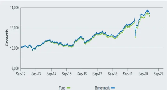
Figure 4. iShares Global Corporate Bond

Notes: development of 10,000 USD over time for iShares Global Corporate Bond UCITS ETF and its benchmark Bloomberg Barclays Global Aggregate Corporate index from Sep 2012 to Feb 2021.

Source: iShares (2021).

2_{Letters are used by State Street Global to identify the fund investor group, where P indicates that it is traded by All}

Investors and I that the fund is traded by institutional investors. SSGA has a State Street Global Treasury Bond Index fund (I) as well. The fund traded by all investors was considered as a better market proxy. Since the Pearson correlation of the log returns for the two funds is 0.99 over the time period, the choice of P instead of I would not make a considerable difference.

(31)

25 31/12/2015-31/12/2016 31/12/2016- 31/12/2017 31/12/2017- 31/12/2018 31/12/2018- 31/12/2019 31/12/2019- 31/12/2020 2020 Calendar Year Fund 4.13% 8.87% -3.37% 11.37% 9.98% 9.98% Benchmark 4.27% 9.09% -3.57% 11.51% 10.37% 10.37%

Table 2. Returns for iShares Global Corporate Bond

Notes: annual returns for iShares Global Corporate Bond UCITS ETF and its Benchmark Bloomberg Barclays Global Aggregate Corporate Index. 12 Month Performance Periods (% USD)

Source: iShares (2021)

As seen in Table 2 and Figure 4, the returns of iShares Global Corporate Bond UCITS ETF and Bloomberg Barclays Global Aggregate Corporate Index are close to identical. Due to this, it is concluded that the fund is a good mirror of the index. Furthermore, some of the discrepancies in the market movements are due to the fact that the values displayed for the fund are the net asset value (NAV) of the fund. The reason why this matters is since the NAV is set after the total expenditure costs are deducted (Avanza, n.d.). The total expense ratio (TER) of the iShares Global Corporate Bond UCITS ETF is 0.20% (iShares, 2021). Due to this, the annual returns of the fund should be approximately 0.20% higher which would bring the returns of the instruments even closer. Thus, the reliability of the fund managers’ capability in tracking the market movement of the index is increased. The fund prices reflect those returns an investor would have received from investing in the index. These are in fact about 0.20% percent lower than the growth of the prices of the underlying asset prices. Thus, the fund prices do not perfectly reflect the returns of the corporate bonds market. However, since a TER of 0.20% is low, this difference is negligible. The regional allocation of the fund seen in Table 3 ensures the suitability regarding global representability. Geographic Breakdown (%) Country United States United Kingdom

France Germany Canada Japan Netherlands Switzerland Spain Australia Other

Percentage 54.39 8.13 6.72 5.03 4.65 2.87 2.49 1.98 1.79 1.76 10.19

Table 3. Geographical distribution of iShares Global Corporate Bond UCITS ETF

Source: iShares (2021).

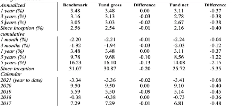
As previously mentioned, the State Street Global Treasury Bond Index Fund (P) was chosen to represent the treasury market. As seen in the column “difference” next to the column “fund gross” in Table 4, the State Street Global Treasury Bond Index Fund (P) closely mirrors the price

(32)

26

movements of the Bloomberg Barclays Global Treasury Index. Thus, the difference in the return of the index and the fund is mainly explained by the TER which is 0.36%. The geographical exposure shown in Table 5 further supports that the fund will continue to be a good mirror of the index. More importantly, the wide geographical distribution makes the fund a good fit as a global representative to the treasury bonds.

Table 4.Performance of State Street Global Treasury Bond Index

Notes: Historical returns of State Street Global Treasury Bond Index Fund and its benchmark Bloomberg Barclays Global Treasury Index.

Source: SSGA (2021) Country Allocation United States Japan United Kingdom

France China Italy German Spain South Korea

Australia Other Fund (%) 26.21 24.42 6.89 6.33 5.95 5.85 4.55 3.60 1.77 1.62 12.80

Benchmark (%) 26.17 24.43 6.81 6.33 5.99 5.89 4.56 3.60 1.83 1.61 12.78 Table 5. Geographical exposure of State Street Global Treasury Bond Index

Notes: Geographical exposure of State Street Global Treasury Bond Index Fund and its benchmark Bloomberg Barclays Global Treasury Index.

Source: SSGA (2021)

3.2.1.3 Stock market

Moving on to the index representing the stock market, the MSCI World Index captures the performance of 1583 constituents of large and mid-cap stocks of 23 developed countries, covering a free float-adjusted market capitalization of approximately 85% in each country. The country which composes the largest proportion of the index is the US which has a weight of 66.11%, followed by Japan (7.74), the UK (4.38%), France (3.39%), and Canada (3.21%). Other developing countries have a weight of 15.17% in the index (MSCI, 2021). The index also presents various sectors such as the IT sector, Financials, and Health Care. The methodology of the index is based