School of Innovation Design and Engineering
Västerås, Sweden
Thesis for the Degree of Master of Science (120 credits) in Computer
Science with Specialization in Software Engineering 30.0 credits
TOWARDS AUTOMATED ANALYSIS OF
EXECUTABLE MODELS
Jean Malm
jmm11001@student.mdh.se
Jonas Skoog
jsg11007@student.mdh.se
Examiner: Björn Lisper
Mälardalen University, Västerås, Sweden
Supervisor: Jan Gustafsson
Mälardalen University, Västerås, Sweden
Technical Advisor: Federico Ciccozzi
Mälardalen University, Västerås, Sweden
Abstract
By utilising graphical modelling languages, software developers can design large systems while keep-ing the architecture simple and understandable. Another benefit of uskeep-ing modellkeep-ing languages is the possibility to automatically generate code, saving both time and reducing human errors in code. In addition, through the usage of well defined and executable models, the system can be tested and analysed as early as during the design phase. Doing so, potential errors in the design can be found and corrected during the design phase, saving time and other resources.
In this thesis we present a method for analysing executable model representations of systems through three steps. First the model is transformed to a suitable format for analysis. The result of the trans-formation is then analysed using analysis tools. Lastly, the result of the analysis is mapped back to the source model.
The developed method was assessed through a proof-of-concept using a transformation from the action language for fUML, an executable modelling language. The target of the transformation was ALF, an intermediate language designed for analysis in the SWEET tool. The analysis of the source was performed in regards to properties of the system, such as program flow and value bounds. Through the proof-of-concept, the proposed method was shown to be a viable option for analysing fUML models.
Table of Contents
1 Introduction 4 1.1 Problem Formulation . . . 5 2 Background 6 2.1 Model-Driven Engineering . . . 6 2.1.1 Foundational UML . . . 6 2.2 Model Transformations . . . 8 2.3 Program Analysis . . . 82.3.1 SWEET and ALF . . . 9
3 Related Work 11 4 Work Method 12 4.1 Designing the Analysis Method . . . 12
5 Analysis Method 14 5.1 Model Transformation . . . 14
5.2 Analysis . . . 15
5.3 Mapping the results . . . 15
6 Proof-of-concept - fAlf to ALF 17 6.1 fAlf as source language . . . 17
6.1.1 Subsets of fAlf . . . 17
6.2 Analysis Using SWEET . . . 18
6.3 Transformation from fAlf to ALF . . . 19
6.4 Mapping between Source and Target . . . 21
6.4.1 Classes . . . 22
6.4.2 Sequences . . . 22
6.4.3 Branching . . . 23
6.5 Analysis with SWEET . . . 23
6.6 Mapping Back the Result . . . 24
6.7 Validating the Analysis . . . 25
6.8 Result of the Proof-of-concept . . . 26
6.8.1 Results from Analyses . . . 26
6.9 Evaluation of the Proof-of-concept . . . 27
6.9.1 Improvements . . . 28 7 Evaluation 29 8 Conclusion 30 9 Acknowledgments 30 References 33 Appendix A Glossary 34 Appendix B fAlf to ALF Mapping 35 B.1 Expressions . . . 35 B.1.1 Constants . . . 35 B.1.2 Unary Expressions . . . 35 B.1.3 Binary Expressions . . . 35 B.1.4 Variable Load . . . 36 B.2 Variables . . . 36 B.2.1 Variable declaration . . . 36
B.3 Assignment . . . 36 B.4 If-Statement . . . 37 B.5 While-Statement . . . 38 B.6 For-Statement . . . 39 B.7 Functions . . . 41 B.7.1 Function Declarations . . . 41 B.7.2 Function Calls . . . 42 B.8 Active Class . . . 42 Appendix C 2D Collision Test 44 Appendix D Valve Example 46 Appendix E Leap Year Calculation 49
1
Introduction
In software engineering, a good design is important as a first step to develop a software system that fulfils all requirements, as well as to mitigate unforeseen issues later in the development. In order to understand and reason about the system at a higher abstraction level, developers utilise graphical modelling languages. The major benefit of representing the design through well-defined models is the lack of ambiguity, as opposed to using natural language descriptions which can be subject to misunderstanding due to different cultural backgrounds [1]. By modelling a system at different levels of abstraction, different types of stakeholders can get the information they are interested in, without unnecessary details.
In order for models to be unambiguous, the functionality of each element needs to be defined properly, in a standardised fashion. One common and widespread modelling language is the Uni-fied Modelling Language (UML) [2].
While models aid stakeholders in understanding the system, they are often considered as just additional documentation overhead, as they do not directly contribute to the implementation. In order to increase the relevance of models and effectiveness of software development, model-driven engineering (MDE) puts greater emphasis on the models and their role throughout the develop-ment cycle. Instead of only using the models as a part of the design docudevelop-mentation, the models can be automatically transformed to concrete implementations. These transformations are made possible through formalised modelling languages with well-defined execution semantics, which in turn enables transformations to program code.
The drawback of using graphical executable models is the added complexity when graphically constructing them. In order to alleviate this issue, graphical languages, such as UML are comple-mented with textual representations. The executable modelling language known as foundational UML (fUML) is for instance accompanied by the textual action language for fUML (referred to as "fAlf" in this thesis1) [3].
While constructing executable models puts more weight on the designers, the resulting benefit can potentially outweigh the overhead [4]. The main benefit of an executable model is the poten-tial of early testing and analysis of the system. By enabling analysis of the system‘s behaviour and performance during the design phase, potential errors and issues can be addressed at the beginning of the development, saving time and resources. This is especially vital in cases where the actual implementation of the system is being generated directly from the fUML specification [5]. One kind of analysis, which is interesting to perform on design models, is static program flow analysis. The flow analysis identifies constraints related to the program flow of the system, such as possible loop bounds, infeasible paths, and branch frequency. These flow facts can then be used to estimate worst case execution time (WCET) and performance bottlenecks of the system. These system properties are especially valuable in real-time embedded systems, where predictability is key for safety reasons. A common example of predictability in real-time embedded systems is the deployment of an airbag where variance in the execution time may have fatal consequences. If the airbag is deployed too early, the airbag will already be deflating as the driver hits it, while if deployed too late, the airbag will not be inflated enough. These tight timing constraints lead to the need of timing analyses.
In this thesis, we present a method for analysing executable models in three steps. The first step of the method is to transform the source model to a format that is suitable for analysis. In the second step the result of the transformation is analysed using established tools. The last step of the method is to map the results from the analysis back to the source model for the designers to investigate. This three-step method can then be used as a template for constructing automated analysis tools of executable models.
In order to test this method, we run a proof-of-concept to statically analyse a subset of the ex-ecutable modelling language fUML through model transformations. By transforming the models into a textual format designed for static verification, we can identify non-functional properties such as the value bounds of the system. The chosen target language for the transformation is the Artist2 Language for Flow analysis (ALF). ALF is designed as an intermediate language used in the SWEET (SWEdish Execution Time) tool for flow analysis, developed at Mälardalen University [6]. In the remainder of the paper, we will begin by presenting the problem formulation of this work. In chapter 2, the background will be presented in three different parts: model-driven engineering, model transformation, and software verification. In chapter 3, we discuss related work for the process in general as well as a few subcategories such as: model-to-text transformation, model verification, and traceability of model transformations. The method used during the course of this work is then detailed in chapter 4. In chapter 5, a specification of the method developed for per-forming analysis on executable models is presented. Afterwards, in chapter 6, a proof-of-concept of the method is discussed in great depth. In chapter 7 and 8, an evaluation of the work is presented along with a summary and conclusion.
1.1
Problem Formulation
Currently there does not exist any method able to perform non-trivial analysis on executable models. A solution to this could potentially reduce development costs by introducing in-depth system analysis early in the development cycle. This work aimed to solve this by developing a method for analysing executable models and testing it by constructing and assessing a translator between a subset of fUML and ALF. By performing this work, the following research questions were answered:
• Is it possible to analyse executable models of a high abstraction level using low-level analysis tools?
• Can the result from the analysis be presented in a way that is understandable by system designers at the design level?
2
Background
In this section, we will discuss the background of this work, starting with model-driven engineering and the benefits it provides to more classical software development processes. Additionally, we will discuss fUML and its textual representation, fAlf. Following MDE and fUML a review of some of the different types of model transformation is presented. The background section ends with a discussion of static verification techniques related to this work.
2.1
Model-Driven Engineering
Developing large and complex software systems can often introduce communication problems be-tween developers because of different interpretations of the design. In MDE, these misunderstand-ings can be reduced through the use of a common, unambiguous way of expressing the design. Models provide a way of describing a system at a higher level of abstraction. The languages used for constructing models are called metamodels. A metamodel specifies concepts and rules to be used for creating well-formed models. By describing the system at a higher abstraction level, mod-els focus more on the problem to be solved rather than the technology to solve it. This allows domain experts to actively take part in the design of the system, to ensure that the developed system meets the user’s needs [7]. The use of well-defined models in the system design also gives the possibility to use model manipulations, so called model transformations in order to generate a partial or complete system implementation.
Aside from generating executable programs, well-defined metamodels provided with a well-defined execution semantics can lead to executable models. Describing an executable model can be tedious if using graphical notations only. That is why executable metamodels often provide the possibility to describe complex algorithmic behaviours through a so called textual action language [8]. These action languages are more similar to standard programming languages and offer an easier way of constructing algorithms rather than graphically modelling them.
2.1.1 Foundational UML
fUML is a subset of UML, for which an execution semantics is defined. The possibility of executing fUML models results in a huge advantage over non-executable models, as the system can be tested through early execution and in-depth analysis. However, executability adds complexity to the models, which can be tedious to define entirely through standard graphical notations. This issue is relieved through the use of the action language for fUML (fAlf), a textual representation of fUML. By mapping the languages together and allowing for automated transformation between the two, a designer can easily design parts of the model graphically while writing complex algorithms in its textual representation, fAlf. An example of this can be seen in Figure 1, which shows a quicksort algorithm in both fUML and fAlf.
Figure 1: fAlf code for a quicksort algorithm, as well as its corresponding fUML model as seen in [9], a modified figure from the official fAlf syntax documentation [10].
As seen in Figure 1, fAlf has a high resemblance with commonly used high-level languages such as C++ and Java. The supported constructs include standard ones such as: variable declaration, functions, assignment, and branch statements. In addition, fAlf also includes object-oriented con-structs like classes, access modifiers and inheritance [9].
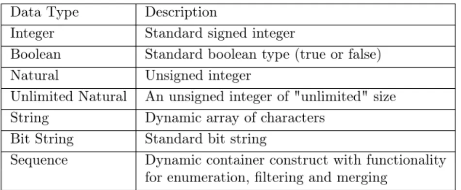
The standard data types that are supported in fAlf can be seen in Table 1. For more information regarding the syntax of fAlf, see the fAlf language specification [10].
Table 1: Standard data types supported in fAlf. Data Type Description
Integer Standard signed integer
Boolean Standard boolean type (true or false) Natural Unsigned integer
Unlimited Natural An unsigned integer of "unlimited" size String Dynamic array of characters
Bit String Standard bit string
Sequence Dynamic container construct with functionality for enumeration, filtering and merging
As for the execution of fUML models, they are separated into three execution semantics as described in the fAlf documentation [10]:
1. Interpretive Execution: fUML models are executed by a modelling tool that interprets its textual representation, fAlf.
2. Compilative Execution: The model is executed according to the semantics in the fUML specification.
3. Translational Execution: The fUML model or the fAlf code is translated into a target lan-guage that is not based on UML, then executed.
In this work, we focus on translational execution. More specifically, we provide mechanisms for transforming a subset of fUML into ALF code for analysis through execution in SWEET. By automating this process, fUML models can be analysed with regards to the previously mentioned aspects and without significant additional effort from the designers.
2.2
Model Transformations
In MDE, model transformations are used for providing automation in terms of automated manipu-lations of models. System requirements can be partially transformed to a design model [11], which in turn can be transformed into another model aimed for analysis and testing [12], and at the later stages of development, models can be transformed to executable programs [13].
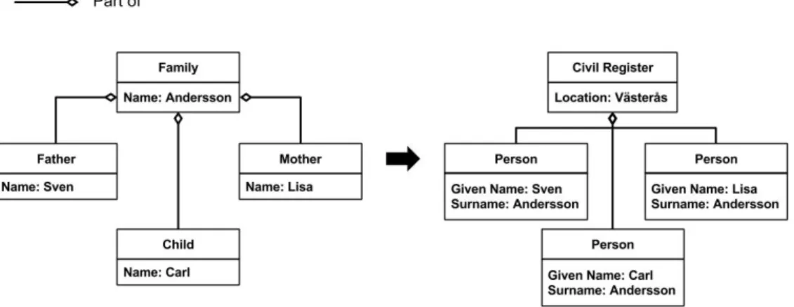
Model transformations come in three forms: model-to-model, model-to-text, and text-to-model. In the first one, both the source and the target of the transformation are models. This kind of model transformation usually transforms the source model from one metamodel to another, thus changing the modelling syntax used, as seen in the simple example in Figure 2. The second trans-formation type is where the model is used to generate some form of textual representation of the model. An example of this could be generating API documents, or even executable code, from the models. Lastly, the text-to-model transformation can be seen as code compilation where the target language is a model instead of machine code, an example is the generation of UML class diagrams from source code.
Figure 2: A model-to-model transformation converting a family model to a civil register model. As this work aims at a translational analysis of models we will take a closer look at some of the approaches for model-to-text transformations. In [14], the author presents two approaches for model-to-text transformations, visitor-based and template-based. The visitor-based approach traverses the elements of the model and writes the produced text to a text stream. The second approach uses templates to access and expand the source model into string fragments [15]. One of the benefits of the template-based approach is that it promotes an iterative implementation as the translation itself can be constructed with a preexisting template as base.
Additionally, as the overall purpose of this work is to analyse the model, it is important to be able to trace the results of the analysis back to the source model. One way of achieving traceabil-ity of model transformation is through ad-hoc intermediate metamodels used to define explicit trace models [16]. These trace models map source and target models through bidirectional relations, resulting in an easy way of tracing in both directions.
2.3
Program Analysis
In software development, the quality of a system is usually ensured through testing and static analysis of the system. The testing of a system is performed by executing its code and comparing
actual outcomes with expected outcomes. Static analysis of a system is instead performed by analysing the source code or a representation of it using some formal method(s).
In this work we focus on program flow analysis on models. This kind of analysis can be used to identify information about a program’s execution. Such properties include: what functions are called, dependencies between conditional statements, and properties of loops such as the number of times it can run. Additionally, by analysing the possible paths of execution, infeasible paths can be identified. Furthermore, by testing the system using all possible inputs (relevant to branch conditions), it is possible to identify and remove dead code.
Similarly, by analysing all of the possible paths of execution coupled with identified properties such as loop bounds, the longest path through the program can be found. By combining this path with timing information of atomic low-level parts of code (instructions) the worst-case execution time of the system can be estimated [17]. However, identifying the timing information of the low-level code is difficult and dependent on the hardware architecture used. In [18], the authors propose a method for identifying these low-level timings through the use of linear timing models. This is done by first constructing a set of training programs for the given source language. These programs can then be executed on hardware, timing the programs. In addition, the programs can also be analysed in an emulator, counting the different instruction calls. By combining the execution times and the calls to different instructions the linear timing model can be identified. Timing of the source language and hardware architecture can then be estimated from the timing model.
2.3.1 SWEET and ALF
A tool for performing flow analysis is SWEET, developed by the WCET research team at Mälardalen University [19]. The tool uses an analysis method called Abstract Execution, which is based on Abstract Interpretation and analyses an abstract representation of the program [20]. Instead of concrete variables having concrete values, the values of abstract variables are intervals, represent-ing all possible values that the variable can have at that point of execution. Abstract Execution uses this information in order to calculate relevant flow facts, such as branch selection and loop bounds [21].
In order to make the analysis independent of the source format, be it a model, code or exe-cutable file, SWEET uses an intermediate language called ALF [22], specifically created for flow analysis. The language itself has a similar structure to C-like languages, meaning that it is an imperative language with global variables and functions. As ALF is designed to be generated from a wide range of sources, meta-information, such as endianness2or the least accessible unit size3is
defined for each program [9].
The ALF data area is divided into a set of frames, each frame having a unique symbolic base address (a name) and a size. This makes it possible to mimic high-level data memory models, by allocating one frame for each variable in the program. These frames can be either globally allocated or local to a function [23]. Since ALF is meant as a flexible language, values are defined both by their value type and by the specified size of the type. There are a number of possible value types:
• Numerical values (unsigned/signed integer, float, bitstring etc.).
– Constants have an explicit syntax that defines type (how they should be interpreted) and size.
– The size inf denotes values of unlimited size.
• Frameref, the base address of a variable. Used when storing data in variables.
2If bit sequences go from most significant bit to lowest or the other way. It an impact on bit operations, for instance shifting in the wrong direction.
• Label reference, the base address of a program label. Used for program flow control instruc-tions.
• Data address, a frameref and numerical offset. Used when loading values from variables. As values in ALF include the size, operators require the size of the operand(s) to work properly. The following are some of the operator types found in ALF:
• Operators on limited size data, includes standard machine-code instructions for arithmentic expressions and comparisons.
• Operators on unlimited size, useful when modelling ”purely” mathematical operations. • Bitstring operators for concatenation and masking.
• Conversion from bitstrings to numerical data. • A load operator to read the value stored in a frame.
The executable code is logically divided into functions, which have their own scope and variables. All functions are declared globally, and like a normal programming language, consist of a number of statements which are executed sequentially. Statements and instructions are written in pre-order, with the operator first, surrounded by curly brackets. The following is a list of the most important statements found in ALF [22]:
• store, which assigns a list of values to a corresponding list of memory locations. Both values and locations are evaluated dynamically and concurrently.
• switch, which is used for conditional jumps. An expression is evaluated and compared to a list of values. Each value has a corresponding target label, and when the first match is found, the execution will jump to that label. A default label can be provided for cases where no values match.
• Function call and return. Call has three arguments: the function to be called, the function‘s parameters and the address in which the returned value should be stored. Return will transfer the execution back to where the function was called and assign the returned value to the address specified in the call statement.
• An unconditional jump, which will immediately transfer execution to the given address. Jumps are normally used for looping.
Program points in ALF are defined using named labels. Since the analysis results are connected to these labels, some care should be taken during naming in order to make the results easier to understand, for example when interpreting back-mapping results.
As ALF is primarily meant to be generated from other sources, it is quite verbose and not very suitable to write by hand. Therefore, some translators have been developed, primarily from C [24] and assembly code [25, 26].
3
Related Work
Since the use of executable models is still a relatively new field, not much has been done specifically for analysing these types of models. In order to perform analysis, some type of transformation is often required, as models usually are expressed at a level lacking information vital to the analysis. For instance, standalone WCET analysis tools expect either executable files [27] or specific low-level representations of the program [6]. In order to use these tools, the model would need to be transformed into the correct format.
In a previous work, the authors have identified a feasible subset of fAlf translatable into the representation used in the SWEET analysis tool, making it possible to perform flow analysis on fAlf code. However, this approach was done by hand using C as an intermediate language, which may introduce restrictions and dependencies on the existing software for compiling C code into SWEET input files. It also lacked a formal source-to-target mapping as well as traceability between the results from SWEET and the fAlf code [9].
Two works that, when combined, could potentially form a toolchain for early analysis of mod-els (specifically fAlf code) are [12] and [28]. The first work transforms fUML via fAlf code to an UPPAAL model, and the second work performs WCET analysis on annotated UPPAAL models. However, for this to be a viable option the output of the first translation would need to be anno-tated automatically. Additionally, the UPPAAL analysis does not scale well, making analysis of non-trivial code infeasible due to long analysis time. The work would also need to be extended to include mapping results back to the original model.
In [29], the process of going from a model to code and then automatically mapping the analy-sis results back to the model is presented. However, the timing analyanaly-sis is done by clocking the actual execution of the generated code, tying it to the underlying system performing the analysis. This is a potential constraint if the system being modelled is meant to run on different hardware configurations, where having a timing model independent of the system performing the analysis may be preferable.
One of the core principles of model-driven engineering is the ability to generate code and/or analysable artefacts directly from high-level models. In [30], a model-to-text transformation is done in order to pass the system specification to a tool for worst-case response time analysis. However, in this work the authors started from MARTE, a modelling language designed for non-functional properties, instead of an executable UML model.
There is a lot of research done in the field of system verification at model level. However, most models are usually either too large and complex, or lacking enough information to be analysed. The general approach is to first transform them in order to take advantage of existing tools [31, 32], or make it possible to combine and analyse information from different model diagrams [33]. As previously stated, for most analysis methods it is not the actual model that is analysed, but a transformed version of the model more suitable for analysis. This makes the ability to map any results back to the source vital, especially when the path from source to target may go through several intermediate steps. Most model-to-model transformation frameworks support some form of automatic traceability, by creating a separate trace model during execution of the transformation [34, 35].
Model-to-text traceability is usually achieved by annotating the generated text with necessary information to find the corresponding element in the source model, for example a unique ID [36]. While the traceability in this case is used for distinguishing between generated and non-generated code, the principle and methods presented can still be applied to this work.
4
Work Method
The work proceeded over the course of five months and was divided into four parts: information gathering, designing the process, implementing a proof-of-concept, and finally evaluating the work. Due to the lack of related research in the field of executable model analysis, the search for relevant background information was expanded to include different subcategories such as model verification, model transformation, and traceability of model transformations.
The background information was found through searching for relevant articles on Google Scholar using the different search strings, such as: "model to text" & (analysis OR testing) & traceability & -"requirements engineering".
From the top search hits based on relevance, an initial screening was done based on their titles and abstracts. Using the articles found, more were then gathered by using the snowball method [37].
4.1
Designing the Analysis Method
The analysis method was designed using the engineering design process [38], a methodical approach to designing solutions. The approach was adapted to our needs which resulted in the following steps:
1. Define the Problem 2. Do Background Research 3. Specify Requirements 4. Create Alternative Solutions 5. Choose the Best Solution 6. Develop the Solution 7. Test and Redesign
As previously stated in the problem definition, the goal was to be able to analyse executable models. Based on information gathered by researching model analysis processes, the following requirements were derived:
• As models are rarely analysed as-is, any transformations done from the source to target must preserve the source model’s logical structure as much as possible.
• In order to get a better understanding of the analysis results, it should be possible to connect them back to the source model.
With these requirements in mind, various alternatives were designed and discussed within the project group. Using the method created for feasibility testing in [9] as a base, improvement ideas were gathered through brainstorming and studying related solutions. The resulting method was achieved through the following steps:
1. Construct an intermediate metamodel to aid traceability and modularity.
2. Implement a model-to-model transformation from the source metamodel to the intermediate metamodel from step 1.
3. Implement a transformation between the intermediate model and the chosen target (code, text, binary etc.).
4. Perform the analysis using a third-party analysis tool.
To test this method, the steps would need to be implemented for some source-target pair and the analysis results will need to be verified with regards to their correctness and assured that they are understandable in the context of the source model. In order to do this, a set of test cases should be created.
5
Analysis Method
In this section, we will first go through a short overview of the analysis method and then take a closer look into each step.
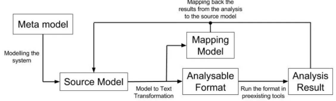
The developed method is a three-step process consisting of model transformations, analysis, and mapping back the results to the system designers, as seen in Figure 3. In the first step, the model of the system is transformed to a format more suitable for existing analysis tools. The transforma-tion itself can consist of one or more transformatransforma-tions depending on the differences in complexity between source and target, desired reusability, and/or multiple target formats.
In the second step, the actual analysis is performed. By transforming to a target format suit-able to existing tools, the second part can make use of established and tested analysis tools. This simplifies the problem by offloading the analysis itself to already functional tools and makes it possible to include various analysis methods through different tools.
The last and final step of the method is to send the analysis result back and present it to the designers. It is critical that the mappings of the result to the source model are presented in a way that can be understood by the designers.
Combining these three steps results in a translational analysis of an executable model where the result is mapped back to the source for easy interpretation of the result.
Figure 3: The analysis method from source metamodel to analysis of the model and back.
5.1
Model Transformation
The first step, consisting of transforming the source model into an analysable format, is the most complex from an implementation standpoint. A transformation can be more easily created by utilising existing concepts in MDE, such as metamodels. These concepts, if available, provide a way of easily traversing the models as opposed to classical text translations, such as compilers, where this is achieved by tokenizing and parsing [39].
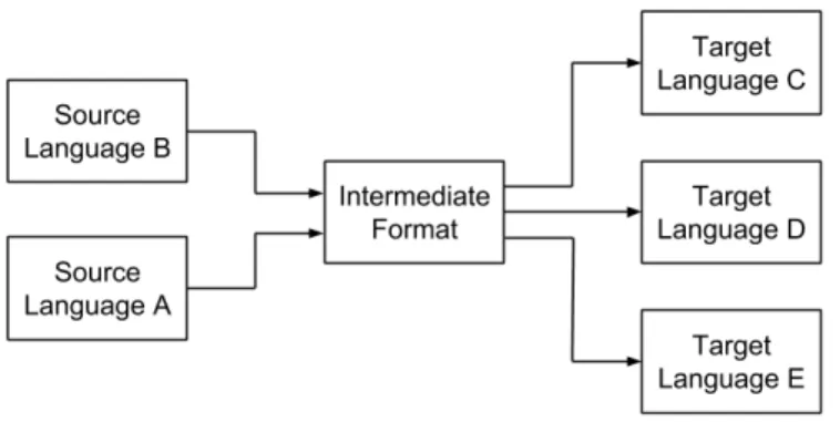
For transformations between languages with a large variance in abstraction level, it can be prac-tical to reduce this difference stepwise through the usage of intermediate languages. The usage of intermediate languages also promotes reusability of the transformation. As a result of utilising an intermediate language between the source and target, we can expand the process to include trans-formations to multiple target formats intended for different analyses (see Figure 4). In addition, it is possible to translate from different metamodels to the intermediate model, thus utilising the already defined intermediate-to-target translations.
Figure 4: By using an intermediate language, different sources can utilise the same intermediate to target transformations.
However, one of the main drawbacks of using an intermediate language is the added complexity and the potential development costs of writing the additional transformations to and from the intermediate language.
In addition to transforming the source model to the target format, this step of the method is also responsible for generating the mapping model. This is done by saving the source element and the corresponding generated element in such a way that it is possible to map back from the generated element.
One of the most important parts of this step is to test and make sure that the generated re-sult is logically equivalent to the source model. Failing to do this would compromise the integrity of the analysis and its result.
5.2
Analysis
For the analysis part of the method, the workload is shifted towards existing tools. The reuse of existing tools makes it possible to utilise different kinds of analyses by translating to multiple end formats.
Among the possible analysis methods, one of great use in real-time systems is WCET analysis, which determines the worst case execution time of a given system, usually by annotating instruc-tions or code blocks with timing information. In addition, using a similar technique, it is also possible to derive a system‘s energy consumption [40]. Furthermore, information about a system‘s value bounds at specific program points can also be obtained through analysis.
One of the main drawbacks of using third-party analysis tools can be the low abstraction level of their input format. This results in a large difference in abstraction level in comparison to the source modelling languages. The difference in abstraction adds complexity for the transformation by having to represent high-level constructs using compositions of low level constructs. Such trans-formations may introduce logical inequivalence between source and target, resulting in an invalid analysis.
5.3
Mapping the results
Due to the use of third-party analysis tools, the result from the analysis tools may or may not be directly understandable to the designers of the system. For example, the result may be presented as data that is not easily interpreted without knowledge of the analysis method itself. Additionally, analyses performed on a low-level format may lead to the results being difficult to understand from a system design viewpoint.
that the system designers can interpret them correctly. Therefore, in the last part of the model analysis method, the results from the analysis part are mapped back to the source model. To map back the result, knowing the relation between source elements and their counterparts in the transformed format is important.
By following the ideas from [34, 35, 36], a traceability model is generated in an appropriate for-mat during transforfor-mation. This model is populated with transforfor-mation data by saving what source element correlates to what resulting element for the given transformation. For example, if an assignment node in the source model is transformed into multiple store statements (some for expression evaluation and one for the actual assignment), the traceability model needs to store which element correlates to which lines of code. By traversing the traceability model, we can then map back information from the analysis to the correct element in the source.
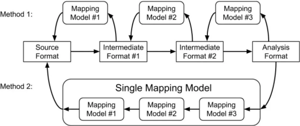
It is important to note that for each transformation, a new traceability model needs to be gen-erated, or the existing model needs to be modified (see Figure 5). Mapping back the results will then include multiple steps, to be performed in the correct order, to match the number of transformations.
Figure 5: Image depicting two different mapping formats, the first consists of multiple mappings while the second merges them into a single format.
Once we have a way to connect the result to the source model, the next step is to present it in a simple and easy to understand way. For reporting the result back to the source, two different ways of presentation were identified. The first is to present the result of the analysis independent of the source, i.e. presenting properties of the system in a separate file. The difficulties with this approach is to make sure that the presentation of the specific program point is understandable by the designer. For example, presenting the program points as low-level labels, as they may appear in the analysis tool, might lead to misunderstandings if the source itself does not contain them. It is therefore important to translate labels into a more readable representation such as the amount of times an if-statement is entered, for instance.
The idea behind the second way is to insert the result back into the source model. This can be inserted as properties in the relevant source elements, such as value bounds in function el-ements. In order to do this, an altered version of the source metamodel, that includes these additional properties, needs to be used. If the designers prefer observing the source as an action language the results may be presented as annotations or comments, displaying the loop bounds of a while-statement for example.
Both methods of presentation may be useful depending on the source language, analysis method, as well as the needs and preferences of the designers. It is therefore important to choose a method on a case-by-case basis and construct the mapping model as independent from the presentation method as possible. This especially holds true when dealing with multiple transformations and/or analyses.
6
Proof-of-concept - fAlf to ALF
As a proof-of-concept, the described analysis method was implemented as a plug-in for Eclipse4
using fAlf action code as the source and ALF as the target, with SWEET as the analysis tool. The results of the analysis were then mapped back to the original fAlf code and inserted as comment blocks. Some results of the fAlf analysis can be seen in appendices C-E where three different fAlf programs have been analysed using the method.
The reasoning for choosing the particular source language and analysis tool was to continue the work done in [9], where the transformability between fAlf and ALF was analysed. In addition, fAlf as a source language has extensive documentation and tool support. As with fAlf, the ALF documentation is also quite extensive and the tool, SWEET, is free to use and provides analyses of interest to early stage development.
The analyses supported in this proof-of-concept are the flow and value analysis. Flow facts, given by the analysis, can be used to identify bottlenecks and infeasable paths. The value analysis gives value bounds for program points, and can be used to identify possible value-related issues, such as division by zero. These kinds of properties are of interest when modelling embedded systems, and would make fUML more applicable in such domains.
The goal with the proof-of-concept is to give an example of how the method can be applied, as well as to test what kind of results can be obtained and reason about the benefits from such an analysis.
6.1
fAlf as source language
The source language chosen for the proof-of-concept is the fAlf language which is an action lan-guage for the fUML modelling lanlan-guage. The lanlan-guage itself can be used to define and annotate behaviours directly into an fUML model, leading to benefits in testability and reusability.
There is some support for development using fAlf, as the Papyrus modelling environment [41] comes pre-loaded with plugins for working with fAlf, such as an editor with syntax highlighting and some semantic verification. This includes the fAlf grammar definition as well as functionality for traversing syntax trees generated from fAlf code files, which is quite helpful for transformation, as the tokenization and parsing is performed automatically.
Aside from tools for creating fAlf code, fAlf can be used for automatic test generation or even simulate execution of UML models to see their behaviour in practice [42]. There is an open-source implementation of fAlf5, which transforms fAlf code to fUML in order to execute it. This is a
useful tool for validating the transformation, by executing fAlf and comparing it to the results of the analysis.
As a model representation of fAlf [10, p. 11], fUML models can also be considered intermedi-ate models in an fAlf-to-ALF transformation. The textual format of fAlf makes creating test cases quicker and the results are likely more understandable from a programmer‘s standpoint while the modelling aspects of fUML makes the source easier to navigate.
6.1.1 Subsets of fAlf
The specification of fAlf provides three different levels of syntactic conformance depending on how many features are needed. These subsets, in the order of size, are:
• Minimum conformance: The smallest subset to be supported. Intended to be enough for writing action code snippets inside UML models. Covers the standard procedural features found in traditional programming languages, standard numeric and Boolean types as well as
4https://www.eclipse.org/
the ability to create sequences (arrays). Minimum conformance also includes object-oriented concepts such as the ability to define and instantiate classes as well as custom data types. In addition, it is also possible to define and create associations between class instances, much like the kind between tables in a database. These associations can have different multiplicities; one-to-one, one-to-many or many-to-many. Different code constructs can also be annotated in order to change the execution behaviour: for instance by marking a loop as parallel, its execution will be parallelised.
• Full conformance: On this level, fAlf provides all the functionality necessary to represent be-haviour in an UML model. Full conformance adds operations on sequences, for example find-ing, adding or removing elements; as well as functionality found in functional programming languages, such as sequence reduction. This level also introduces asynchronous execution, where signals can be sent, waited for and received by different threads of execution.
• Extended conformance: This level introduces all the structural modelling possible in fAlf, which is useful for compartmentalising the code into logically cohesive parts. This includes defining and importing packages and namespaces.
For a full description of both conformance levels and of fAlf constructs in general, refer to [10]. For this proof-of-concept, we provide analysis for a subset of the minimum conformance. This choice of subset is due to time constraints, as well as restrictions of the analysis tool.
6.2
Analysis Using SWEET
The tool chosen to perform the analysis is SWEET, a research prototype which performs static analysis of programs using abstract execution [19]. SWEET performs several analyses, including flow analysis to derive loop bounds and infeasible paths [43]. By annotating instructions with a time cost, SWEET is able to derive BCET/WCET data. It can also perform a value analysis which shows the possible values of variables at specified program points. The source code is available on demand, but SWEET can also be run online, making it quite an accessible choice [6].
Most analyses have customisation options depending on the user’s needs. As an example, flow facts can be generated both for single nodes and node pairs. The first one is interesting for loop bounds, as it can be used to tell how many times the loop body has been entered, while the second is useful to find infeasible paths (if for all potential inputs, execution path from node A to node B is never taken). Using additional annotations, it is possible to override values of frames in specified program points. This can for instance be used to run the program using a specified range of inputs. The SWEET analysis tool has some restrictions on what it can analyse, which has an impact on what was translated:
• SWEET does not support recursion, so recursive algorithms will need to be transformed into iterative algorithms.
• SWEET cannot handle dynamic memory allocation. • SWEET currently cannot handle parallelism.
• The analysed program must terminate in order to produce analysis data. • The analysis performed by SWEET must terminate6.
ALF, the intermediate language used in SWEET, is an imperative language with a mix of high-and low-level statements [22]. This means that while there are dedicated statements for structured function calls and switch-case, instruction-level statements are also available. However, it has no
6The analysis performed in SWEET may not terminate for certain programs. The reason for this is that SWEET uses overestimations for possible values of variables. In rare cases, this leads to that analysis of loops do not terminate properly during analysis.
support for object-oriented classes and constructs. A more in-depth description of ALF can be found in section 2.3.1 or in [22].
As a consequence of ALF being meant as a generic language for flow analysis, it is actually possible to model programs using ALF that cannot be analysed by SWEET. For instance allocating and freeing dynamic memory using dyn_alloc and free are perfectly valid in ALF, while not supported by SWEET.
6.3
Transformation from fAlf to ALF
The model-to-text transformation was implemented using Xtend7, which is a ”dialect” of Java with
powerful text formatting functionality, making it well-suited for text generation. However, in order to generate code from the source model, functionality for traversing the model is necessary. For this purpose, Xtext8 was used, which is a framework for creating custom textual languages that
supports traversing and retrieving information from the language‘s syntax tree. The reason for choosing Xtext is that the fAlf grammar is already defined in Xtext, which saves a lot of develop-ment time.
For each node type in the syntax tree, a corresponding “compile“ function was created, which generates ALF code from the given node. A visitor-based translation method was then applied that recursively traversed the tree from the top. For each node, the correct compile rule is applied, generating well-formatted text using the text formatting functionality of Xtend. Once the entire tree has been processed, the result is written to a file for further processing or analysis.
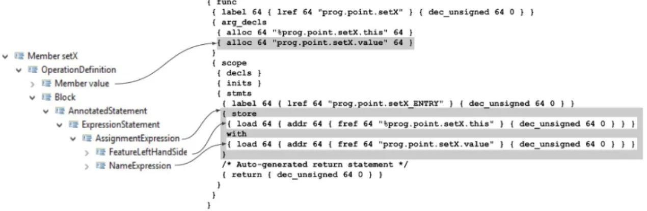
To properly translate between fAlf and ALF, information about the current scope had to be kept track of during compilation. In fAlf variables can be declared anywhere within a function body. ALF instead has a dedicated block for local variable declarations. This meant that every time a variable declaration statement was compiled, information, such as size and type of the variable was added to a list. From there, it could later be retrieved in order to fill out the ALF declare block after the entire function had been compiled. For example, the string format for function definitions can be seen in Figure 6 and a concrete example of the result can be seen in Figure 7.
7http://www.eclipse.org/xtend/index.html 8https://eclipse.org/Xtext/
Figure 6: The Xtend formatting string for function definitions in ALF. Format strings start and ends with ” ’, and everything in-between is formatted verbatim, unless written inside «», in which case it is evaluated as a string and then inserted. As seen with the addDefaultReturn flag, condi-tionals can be used inside the formatting.
Figure 7: Example of a simple set function on a 2D-Point class, on the left side we see the function‘s tree structure, while the right side shows the generated ALF code.
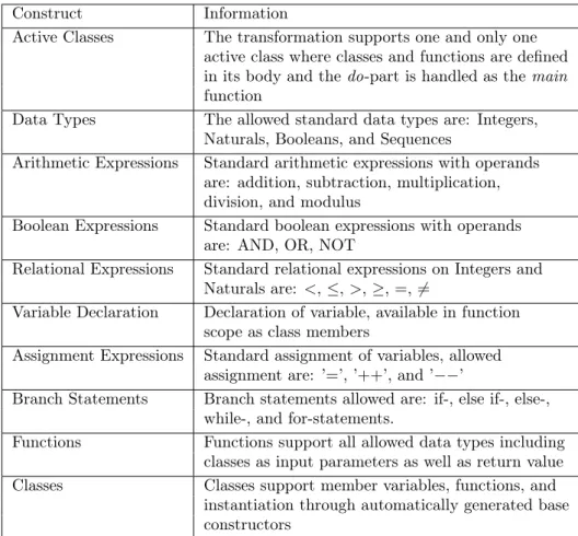
Considering the aforementioned limitations on SWEET and ALF, the transformation was limited to a subset of the minimum conformance level of fAlf. Due to time constraints, some parts were skipped, such as inheritance and defining constructors. Additionally, as an example, while the string datatype is part of the minimum conformance, since ALF does not define any I/O operations and any other usages could be done with more suitable datatypes, strings were excluded. The complete subset supported can be seen in Table 2.
Table 2: Supported subset of fAlf. Construct Information
Active Classes The transformation supports one and only one active class where classes and functions are defined in its body and the do-part is handled as the main function
Data Types The allowed standard data types are: Integers, Naturals, Booleans, and Sequences
Arithmetic Expressions Standard arithmetic expressions with operands are: addition, subtraction, multiplication, division, and modulus
Boolean Expressions Standard boolean expressions with operands are: AND, OR, NOT
Relational Expressions Standard relational expressions on Integers and Naturals are: <, ≤, >, ≥, =, 6=
Variable Declaration Declaration of variable, available in function scope as class members
Assignment Expressions Standard assignment of variables, allowed assignment are: ’=’, ’++’, and ’−−’
Branch Statements Branch statements allowed are: if-, else if-, else-, while-, and for-statements.
Functions Functions support all allowed data types including classes as input parameters as well as return value Classes Classes support member variables, functions, and
instantiation through automatically generated base constructors
6.4
Mapping between Source and Target
Mapping basic fAlf statements to ALF can be seen as a non-optimising compilation from a high-level language to instruction code. For instance, assigning a value to a variable is fully supported using the store instruction, which expects an address and a value to store. Variable addresses can be retrieved using the addr instruction and their value can be loaded using a load instruction. As can be seen in Table 3, every instruction also requires the size of the argument(s) to be provided, so here X and Y are 64-bit variables.
Table 3: Simple transformation example. The variable X is assigned to the value of Y. fAlf ALF
X = Y; {store /*assignment*/
{addr 64{fref 64 "X"}{dec_unsigned 64 0/*offset*/}} /*Address(X)*/ with
{load 64{addr 64{fref 64 "Y"}{dec_unsigned 64 0 /*offset*/}}}/*Value(Y)*/ } /*End of assignment*/
One thing that is apparent in Table 3 is that ALF code is much more verbose than fAlf, and less readable. In order to avoid having a large number of complex statements in the ALF code while working with the translation, expressions with at least one operator are compiled and the result is stored in a temporary variable, which then replaces the expression. This has the added benefit that the value of sub-expressions can be checked when debugging the ALF code, just by checking the value of that temporary variable. It is also useful when taking compiler optimisation
into account during analysis, as storing and reusing expression results is a useful optimisation. In order to ensure that temporary variables cannot overlap with an actual variable all extra variables generated during the translation have names that are illegal in fAlf, such as starting with a "%" character.
In the following subsections, we will discuss the mapping between certain constructs in greater detail, for a more concrete mapping, see Appendix B.
6.4.1 Classes
In order to create class instances, it is important to know how much data needs to be allocated for them. When a class is defined, information about all its data members such as the name and address offset from the start of the class data is stored. By going through all data members, the total size of the class instance can be calculated and stored for further use. A base constructor is automatically created for the class, which sets all data members to their initial value. Member functions are compiled as regular functions, which take a pointer to the calling object as an extra argument, which becomes the this reference found in standard object-oriented programming lan-guages.
When accessing a class member variable, its address offset is retrieved from the info about the class. The offset is then added to the base address of the class instance in order to get the correct address. For example, for a class having two variables, the address to the second will be the base address plus the size of the first variable, as they are stored directly after each other.
For this address calculation to work, class variables are generated as compositions instead of aggregations, meaning that members that are themselves classes are ”flattened”, instead of being pointers to real objects. The downside of this is that with composition, class instances cannot share the same data, and changing one instance will not affect the other. In addition, the class needs to be defined before it is used as a type. On the upside, the value analysis will be more informative if class instance objects use composition for everything. If association was used and the reference was reassigned at any point, that value would be indeterminate in the analysis result. In SWEET, this manifested itself as the value being shown as undefined, using either the top or bottom constants instead of an actual address.
What is also worth to mention about accessing class members is that checking accessibility is handled at model level, and ALF has no concept of public or private variables, so this can safely be ignored during the translation process.
Lastly, although there is currently no support for inheritance in this particular translator the same general method as proposed in [9] would most probably work. Overriding of methods would be solved by calling them through function pointers, while member variables would be handled using composition.
6.4.2 Sequences
Sequences in fAlf need to get enough space to fit, so their size needs to be known at generation time. There are two different ways of declaring a sequence, either as an inclusive range between two integers, or by providing the concrete list of elements. In the list example, calculating the size required is simple as the elements just need to be counted. For a range declaration, the translation currently requires the lower and upper values to be constants, as it is the only way to ensure that the size will be correct at the time of translation. To keep track of the sequence size, this information is stored in the beginning of the data area.
As previously stated, class member variables are allocated using composition. Sequences how-ever are an exception to this rule, instead being stored as references. The reason is that when declaring the class there is no way to tell how large the sequence needs to be, aside from giving it a static size. This means that when accessing sequence elements from a class member variable,
an extra level of load instruction must be generated to get the actual element, instead of just the address.
6.4.3 Branching
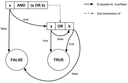
fAlf has two kinds of loop constructs, for and while. While-loops iterate while a condition is true, however for-loops in fAlf specifically iterate over a sequence (usually called for-each), each instance assigning a loop variable to the current element in the sequence. To know when to stop iterating, a temporary variable is generated and used to keep track of the current index.
Considering fAlf uses lazy evaluation for the conditional-and and conditional-or, this needs to be taken into account during the translation. Lazy evaluation means that a conditional-or expres-sion will only evaluate both sides if the left one is false, while a conditional-and will only evaluate both if the left one is true, as seen in Figure 8. Conditional expressions are essentially compiled to a sequence of switch-statements, each evaluating different clauses of the expression, in correct precedence order.
Figure 8: Statechart diagram of lazy evaluation of an expression where x, a, and b can be seen as Boolean variables or hidden sub expressions.
6.5
Analysis with SWEET
Once the fAlf code has been translated into ALF code, it can be analysed using the SWEET tool. The proof-of-concept was limited to two types of analyses, namely flow fact generation and value analysis. The flow fact analysis was done to generate both upper and lower bounds on single node pairs. This means that for each label in the program, the program will count how many times the execution has reached it. Flow facts give important information about the code execution and hopefully allow for interesting observations to be made. The value analysis will try to constrain the possible values of a variable for every label in the program. It can be used to verify that variables are within expected intervals during execution.
As SWEET is the only analysis tool used, the scope of what can be modelled and analysed is limited by what SWEET can handle. This means that workarounds for issues such as rewriting recursive algorithms or finding ways around using dynamic memory will need to be taken into ac-count during the transformation process. It is important that these workarounds affect the analysis result as little as possible.
6.6
Mapping Back the Result
For the last part of the translational analysis, the result from SWEET was mapped back to the source in a format understandable to the system designers. In order to do this, the relation between source element(s) and result element(s) was recorded. This traceability information was then used for mapping results to corresponding source model elements.
In the case of our transformation between fAlf and ALF, the mappings from the source turned out to be difficult. The reason for this was due to using the model representation of fAlf, fUML, as a means for traversing the source. While this gives an easy way of traversing the modelling elements of the source, it results in difficulties extracting information regarding its textual representation, such as line numbers for specific elements. In order to solve this, program points relevant to the analysis were mapped to their respective textual position through parsing the code in a second pass. In addition, variables were also included in the mapping format, connecting their fully qual-ified name in the source with the generated variable names in ALF.
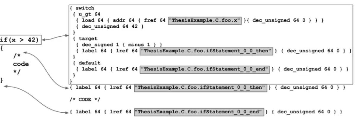
Since the mappings from fAlf were tied to program points, the generated labels were structured based on their fully qualified names. As such, function elements in fAlf would generate a label in ALF code using the following format: ‘ProgramName.ClassName.FunctionName‘, see Figure 9. This would later not only help with the traceability from ALF to fAlf but also with connecting the actual result from the analysis to the mapping format as they would be in a similar form.
Figure 9: A simple if-statement in fAlf with its generated ALF code, note the highlighted entry and exit labels for the if-statement which indicates the first if-statement in the foo function of class C.
The mapping process from result back to the source started by associating the output from SWEET with the end format from the transformation (ALF). First the output had to be parsed and converted to a format suitable for mapping and presenting. The format of the result consists of flow facts and value bounds at program points, a piece of the value analysis can be seen in Figure 10. This information was then mapped back to the correct program points in the fAlf code using the generated mappings. In addition, the variable names were translated back to their original namebindings using the stored variable mappings.
Figure 10: A snippet of a result given by the value analysis in SWEET. The highlited parts are the program point label and the variable label with its value bounds.
As the mappings connected textual positions in fAlf to program point labels in ALF and results were stored using ALF labels as identifiers, the analysis result could be presented to designers. The final presentation format can be seen in the fAlf code in Figure 11, as well as in the relevant appendices. The benefit from this form of presentation as opposed to a separate analysis format is the direct relation between the result and the source code, instead of having to manually associate certain program points with data in the analysis result.
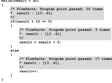
Figure 11: A code snippet of an analysed fAlf program where the highlighted comments show the analysis result.
In Figure 11, we can see that the value of result is greater or equal to 13 before entering the loop. We can also see that the if-body was entered 3 times, and the else was entered 17 times, which in turn matches with the number of times the while-loop was executed. In this simple example, we can also see why the first if-body was entered the given amount of times due to the value analysis of the result variable and the simple logical expression. When dealing with more advanced systems, this kind of information can be vital in order to find errors and to be able to reason about the system design.
6.7
Validating the Analysis
In order to validate the analysis, multiple example programs in fAlf were produced with the in-tention of testing analysis of specific fAlf constructs. By creating multiple examples for constructs such as assignments, branch-statements, data structures, classes, the testing of analysis could be aimed at specific problems. To execute fAlf code as a stand-alone program, an fAlf active class was defined as the top-level element for the transformation. Inside the active class, other classes and variables were defined, and the behaviour definition became the entry function of the program,
akin to the main function in most C-like programming languages.
These examples were then combined to form a testing suite to be used for continuous testing as both the analysis and the suite itself expanded. Unfortunately, the testing could not be easily automated due to how SWEET presents the information from the analysis. Instead, after a test had been run, the source was manually observed to see if the flow and value analysis match with the expected result.
6.8
Result of the Proof-of-concept
The proof-of-concept used the three-step analysis method of fUML models, expressed in the action language fAlf, that follows the method proposed in this thesis. First the fAlf source is trans-formed into ALF while at the same time generating mapping between the source and result. The transformation traverses the source as a syntax-tree in fUML using Xtend. For each element a transformation rule is applied and an ALF program is systematically constructed.
The resulting ALF code is then analysed in SWEET, generating facts about the system such as flow constraints and value bounds of variables. The chosen analyses are flow analysis and value analysis. These two analyses were chosen due to their relevance in embedded systems as an at-tempt to increase the application domain of fUML.
The last step was to map the result back from SWEET to the fAlf source. The mapping in-formation, generated by the transformation and a second pass on the fAlf code, contains the fAlf program points as line numbers in relation to program labels in ALF. In addition, the mapping also contain the translation of variable names in order to present the value analysis results. Using this mappings, the result given by SWEET were mapped back to the source and parsed into a suit-able format. The end result of the analysis were system properties (flow facts and value bounds) injected as comments in the fAlf code.
This proof-of-concept was then tested on multiple examples in order to test the transformations correctness and if it caused potential problems in SWEET. Some of the example analyses on fAlf code can be seen in section 6.8.1 below.
6.8.1 Results from Analyses
During the development of the proof-of-concept, multiple minor examples were constructed for specific program constructs in order to conduct continuous testing. This meant that when a new construct was allowed in the transformation we could run the old examples to see if the old con-structs were still translatable. Apart from these minor examples that tested the transformation, larger examples containing combinations of different constructs were used in order to test their cooperativeness. In addition, these examples were used to test and reason about the analysis per-formed on the source code.
While multiple examples where constructed and analysed, the ones we chose to present in this paper are the examples in Appendices C-E. These particular examples where chosen due to three different aspects. The first is the different constructs used in the examples in order to cover the allowed subset. The second is their simplicity from a presentation standpoint and the last is how interesting the results were.
The first example tests collision between rectangles in two dimensions, as seen in Appendix C. The example combines constructs such as classes, sequences, and for-loops by filling a sequence with rectangles and checks if they collide with each other through a for-loop. By observing the example, we can see that a total of 6 collisions is found by observing the flow facts of the if-statement in the main function. In addition, we can also see that the lazy evaluation is in effect as the innermost while-loop is passed 15 times but the function CollidesWith is only called 10 times. This is as much as we can infer from the example as we limited the displayed analysis to flow facts.
The reasoning for this is due to the inadequate result yielded from the value analysis. The issue being the lack of bounds given to class member variables, resulting in values mostly displayed as top and bottom. While we have not been able to pinpoint the cause of this issue, we believe it to be related to flattening out classes as a large data area in combination with the layers of references used for classes in combination with sequences.
The second example, Appendix D, attempts to emulate a simple pressure control system. This is done through two main functionalities, first a class, PressureSensor, that acts like a sensor, calcu-lating and returning the current valve pressure on demand. The second part is a update function, UpdateValve, that opens or closes the valve depending on the current and desired valve pressure. By analysing the example, we can examine the results injected as comments and in turn infer how the system will behave in the given context. According to the flow facts seen in the UpdateValve function, the pressure needs to be raised more times than lowered, suggesting it starts at a lower level than desired. Using this information, and knowing the control system maintains a desired pressure by oscillating, we can observe that the system will reach a stable state around the 100 cycle mark. This observation is based on the fact that it spends 2 ∗ 26 cycles on oscillating, and is run a total of 150 cycles.
As a general observation on functions, the analysis does not seem to generate a lower bound for the number of times the function is executed, even though this particular example was kept completely deterministic for the analysis. This is most likely not a problem, as this information can be obtained by adding together how many times each mutually exclusive path has been executed. Aside from the observations on the program’s behaviour, we can also observe some aspects of the analysis from this example. For instance, in the if-statements in the Min and Max functions, we can see that the value analysis is able to limit the value bounds inside the else-statements even though they are never passed.
Appendix E shows the results of analysing an example program that counts the number of leap years between two given years. Being a rather simple program, it is easy to understand while still covering most of the fAlf constructs that are supported in the implemented translator, such as assignments, branching and function calls. The analysis was run using the range [1885, 1992] for the start year and [2017, 2042] for the end year. By observing the resulting flow fact annotations, we can see that the while-loop is entered between 26 and 158 times, which seems valid: the value of currentyear is the interval [1885, 2042], the number of integers in the range [a, b] = b − a + 1, so there are 2042 − 1885 + 1 = 158 years to check. However, the remaining flow facts shown are not as exact. As a leap year occurs roughly once every four years, the if-statement in the loop should be true between 6 and 39 times, however the resulting flow fact shows a significant overestimation of [0, 156].
6.9
Evaluation of the Proof-of-concept
Through the proof-of-concept, we can see that it is possible to perform static analysis on executable models using our method of translational analysis. The benefits of such a tool could increase effi-ciency in designing software systems by identifying errors and bottlenecks early in the development cycle.
Despite the benefits of an automated model analysis, the current version suffers from some limi-tations caused by the implementation. Aside from general improvements to the toolchain, such as better and more optimisation of the generated ALF code, there are some specific limitations iden-tified. The first of these limitations is the way self-referencing through the this keyword is handled in combination with the analysis. As the self-referenced instance is handled as a reference, the resulting analysis encounters problems when a member function is called from different instances. This results in ambiguities when trying to derive self-referenced variable bounds in member func-tions.
This is believed to be a result of representing classes as data areas in combination with the refer-encing that happens through sequences and the self-referrefer-encing in functions.
Another observed problem is the potential information bloat that occurs when multiple variables are declared before a given program point. The result from this is that, for each relevant program point, the value bounds for all active variables are printed. The desired effect would be to only present relevant variable bounds such as the variables that are read or written in the scope. The issue with reporting all the active variables is that a lot of information will be repeated while not necessarily changing between program points.
Further issues with the proof-of-concept are the wide bounds given by the analysis when setting value ranges on variables using annotation files when analysing in SWEET. A potential reason for this could be due to some oversight in the transformation, resulting in difficulties limiting the bounds during analysis.
The final identified limit of the toolchain is the time it takes for SWEET to perform its ad-vanced value analysis. This results in difficulties when utilising references in the program code as the simple and quick analysis does not provide precise enough estimations on the value bounds. However, it is not yet identified if this is because of the analysis or the transformation itself. In case of the latter, the generation of the ALF code itself could be adapted to remove these issues. 6.9.1 Improvements
As indicated by the identified limitations of the toolchain there is a lot of space for improvement. One of the more general improvements would be to introduce additional compiler optimisations for the transformation, in order to give faster and more precise analyses.
Additional improvements would include an increase in the supported subset of the fAlf trans-formation, such as class inheritance and dynamic sequences. In the case of the latter, even though SWEET does not allow for dynamic memory allocations, sequences could theoretically be dynamic by allocating a max size for the sequence at compile time. Fortunately, this approach would not restrict the analysis as the memory size used has no effect on the result of the analysis.
A final improvement would be to tailor a new intermediate metamodel specifically for high- to low-level transformations. This intermediate metamodel can reduce the complexity of the trans-formation to ALF. In addition, using this intermediate metamodel, it should be easier to transform fAlf into other low-level analysis formats, or other modelling languages into ALF for analysis in SWEET.