Investigating the change in academic performance of university level
students after a sudden switch to digital education due to the
COVID-19 outbreak.
The Impact of Digitalization on
Student Academic Performance
in Higher Education
Case of Jönköping International Business School
BACHELOR THESIS WITHIN: Economics
NUMBER OF CREDITS: 15
PROGRAMME OF STUDY: International Economics
AUTHORS: Dina Tinjić and Meliha Halilić
Bachelor Thesis in Economics
Title: The Impact of Digitalization on Student Academic Performance in Higher Education (Case of Jönköping International Business School)
Authors: Dina Tinjić and Meliha Halilić
Tutor: Anna Nordén
Date: 2020-08-04
Key terms: Undergraduate Education, Quantitative Study, Field Experiment, Treatment Effect Model, Covid-19, Home-education
JEL: A22, B23, C93, C21
Abstract
As in any other sector, the Covid-19 outbreak has caused many changes in education, and there is a reasonable expectation for this intervention to have a significant impact on the students and their performance. The purpose of this study was to analyse the effects of the digital semester, imposed on students due to Covid-19 outbreak, on student academic success. Using a quasi-experimental methodological approach called dif-in-dif analysis, three empirical models were constructed to analyse if there is an overall effect when comparing our control and treatment groups, as well as if there were any group-specific differences when it comes to the performance across genders and educational levels. The study found a significant negative effect of the digital semester on student academic success, suggesting that students performed significantly worse after the Covid-19 outbreak caused the University to step away from face-to-face teaching and adapt to remote studies. Furthermore, it was found that gender-specific differences do not affect the academic performance of our treatment group; however, female students performed worse when the digital semester was implemented compared to the control group who had both the classes and exams face-to-face. Lastly, Master students were found to perform significantly worse compared to Bachelor students’ when the Covid-19 outbreak caused the education to transfer to the digital environment.
Table of Contents
1
Introduction ... 1
2
Literature Review ...3
2.1 Education and Economic Growth ... 3
2.2 Digitalization in Education ... 6
2.3 Covid-19 and Education ... 10
3
Hypothesis Formulation ... 11
3.1 Hypothesis 1 ... 11
3.2 Hypothesis 2 ... 12
3.3 Hypothesis 3 ... 12
4
Methodology ... 12
4.1 Data Sources and Description ... 12
4.2 Empirical Strategy ... 13
4.3 Test Instruments ... 16
4.4 Construction of Empirical Models ... 16
4.4.1 Model 1 ... 17
4.4.2 Model 2 ... 18
4.4.3 Model 3 ... 19
5
Results and Empirical Analysis ... 20
5.1 Descriptive Statistics ... 20
5.2 Research Question 1 ... 21
5.3 Research Question 2 ... 22
5.4 Research Question 3 ... 23
5.5 Interpretation of R2 ... 24
6
Discussion and Limitations ... 25
7
Conclusion ... 27
8
Reference List ... 30
1 Introduction
The global effect of COVID-19 has created an unexpected opportunity for social scientists to study a natural experiment where the behaviour of people is reflecting real life due to its natural setting. Many questions on its effects are the motivation behind a continuous number of research papers in progress looking into its impacts on different segments in the economy. As in any other sector, the Covid-19 outbreak has caused many changes in education, and there is a reasonable expectation for this intervention to have a significant impact on the students and their performance. Following the government recommendations, many educational institutions around the world have temporarily switched to digital learning methods, to contain the spread of the COVID-19 pandemic. According to the latest updates (UNESCO, 2020), this corresponds to over 91% (1.6 billion) of total enrolled learners globally who got affected by this abrupt transition. As of March 17th, 2020, all teaching at higher education in Sweden has also been transferred to remote studies (Government Offices of Sweden, 2020).
Jaime Saavedra, the Global Director of the World Bank Group’s Educational Globe Practice, referred to the COVID-19 impact as “one of the greatest threats in our lifetime to global education, a gigantic educational crisis”. Such an abrupt transition to remote studies, with a corresponding change in examinations and assessments, has never happened in the history of education. Universities and schools had to adapt to such a change by avoiding face-to-face teaching and implementing an online style of education, as this is seen as the only viable alternative during the times of a global pandemic. Since human capital is an important drive of economic growth, as later discussed in our literature review, pausing the education worldwide, or disrupting the learning environment potentially creates a chaotic situation for the educational institutions and students. On average, more than half of GDP growth in OECD countries between 2000 and 2010 was related to labour income growth among tertiary-educated individuals (OECD, 2012). Moreover, annual labour costs increase substantially with educational attainment, individuals with upper secondary education cost on average USD 46,000 to employ while individuals with tertiary education cost USD 68,000 per year (OECD, 2012). Those findings show the significance of increasing attainment levels as well as earnings that follow with higher educational attainment on growth and prosperity in OECD countries.
Considering the sudden influence of the pandemic, and its impact on educational institutions and the students, we decided to investigate the effects deeper, as it raises many interesting questions. Thus, the purpose of this study is to measure the effects of digitalization, imposed due to COVID-19, on students’ academic success. Analysing student grades, which are used as a reflection of academic success, is one of the easiest ways to obtain such an assessment which is the objective of this paper. Conducting such an analysis, and using the later described model, we focus on measuring and determining the overall effect of digital teaching due to the Covid-19, as well as the group-specific effects across genders and educational levels. Hence, this research investigates the following three questions:
1) What is the overall effect of such an unexpected and sudden switch from face-to-face to digital learning on university students’ academic success?
2) Does the impact of the digital semester affect the academic performance of male and female university students differently?
3) Which tertiary educational levels may be less or more affected by the digitalization of education imposed by Covid-19?
The remainder of this study is organised as follows: section two illustrates the theoretical aspect of quality of education on the economy; how digitalization in education has influenced students so far; as well as the potential influence the Covid-19 outbreak might have on students. In section three, we develop our hypotheses for the three research questions that this study is focusing on. Section four explains our methodological approach to such an analysis, where the data, models, and tests are explained in further detail. In section five, we present our descriptive statistics tables, results, and empirical analysis. In section six, we discuss the results and their potential implications, as well as how they relate to research done so far. Lastly, section seven brings out our conclusion, potential limitations of our research, and suggestion for further research followed by a list of references and appendix, where the data and robustness check for the models is presented more thoroughly.
2 Literature Review
The quality of education is assumed to differ between online and face-to-face studies; therefore, we start by discussing the importance of educational quality and its effects on individual productivity and earnings (microeconomic impact) and economic growth (macroeconomic impact). Next, we present findings of the most prominent studies comparing student academic performance in online versus face-to-face finance and economics courses. Lastly, we include research findings of recent articles and working papers that, similarly to our study, looked into how a sudden switch to online education, due to Covid-19, impacted university students and their grades.
2.1 Education and Economic Growth
Human capital is defined as “the skills, knowledge, and experience of a person or group of people, seen as something valuable that an organization or country can make use of” (Oxford University Press, u.d.).
Education plays an essential role in promoting economic growth for many reasons (Mankiw, Romer, & Weil (1992); Romer P., (1990); Benhabib & Spiegel, (2005)). Most notably, it can increase the human capital in the labour force which boosts labour productivity. Additionally, it can increase the economy’s innovation capacity which in turn leads to knowledge of new and more efficient technologies, processes, and products. Furthermore, it enables the diffusion and transmission of knowledge which is essential in understanding and implementing such new technologies and processes. On a micro-level, higher productivity translates into higher wages.
Harris, Handel, & Mishel (2004) reviewed the existing evidence regarding the general relation between education and worker productivity and found that early studies focused on effects of an additional year of schooling (quantity of schooling) on future earnings since based on economic theory, wages were assumed to be a valid measure of productivity. However, worker productivity was in fact found to be determined by their ability to learn their jobs, which to some extent is determined by general cognitive skills. Cognitive skills, as measured by standardized tests, is now increasingly considered to be the most important measure of educational outcomes and quality (Hanushek & Kimko (2000); Hanushek E. A. (2002); Hanushek & Wößmann (2007)). Educational quality has been identified as an important contributor to individual earnings, the distribution of income, and economic growth (Hanushek & Wößmann, 2007).
The relation between schooling quality to economic outcomes can be measured using two empirical approaches, including a cross country analysis and an individual level analysis. The cross-country analysis focuses on returns at the economy-wide level and is based on observations of economic growth and test scores across countries while the individual level approach measures returns at an individual level using longitudinal surveys to compare test scores with later education, employment and wage outcomes (Deloitte Access Economics , 2016). Since the data we are using in this study consists of individual academic performance rather than that across countries, we will mainly focus on the returns of quality of education on individual earnings, i.e. the micro-level perspective. It should be noted, however, that the literature focuses relatively more on the macroeconomic impact since the “relationship between measured labour force quality and economic growth is [perhaps] more important than the impact of human capital and school quality on individual productivity and incomes” (Hanushek., 2002, p. 9). Direct investigations of cognitive achievement find that, after allowing for differences in quantity of schooling and other control variables that may otherwise impact earnings, measured cognitive achievement, i.e. results on test scores that determine quality, has a direct impact on individuals productivity and earnings, with returns ranging from 4 to 16% (Harris, Handel, & Mishel, 2004). Murnane, Willett, & Levy (1995), for example, used data from longitudial surveys containing information on the labour market performance of students who graduated from high school in 1980. They found an increase of one standard deviation in maths test scores, which was used as their measure of cognitive skills, to be associated with a earnings return of 7-12%. Many other studies in this field focused on earnings differences between black and white skill differences and/or with a focus on males (O'Neill (1990); Neal & Johnson (1996); Murnane, Willett, Braatz, & Duhaldeborde (2001)). O'Neill (1990) used the National Longitudinal Study (NLSY) of more than 12,000 students born between 1957 and 1964 and a qualifications test was administered to 90% of the students as a measure of basic cognitive skills (and determinant of quality). Additionally, students were tracked over time to determine their experiences at work. His findings reveal that an increase in one standard deviation in the qualificatrions test is associated with a 4-5% increase in earnings. Neal & Johnson (1996) used the same NLSY and found a substantially larger increase in earnings of approximately 20%. The difference in results is based on differences in subsamples used and regression specifications. Notably, Neal & Johnson (1996) used fewer explanatory variables and found that when quantity of schooling is added back into their prefferred specifications, the size of the estimate is reduced from 20% down to 12-16%. Murnane, Willett, Braatz, &
Duhaldeborde (2001), using the NLSY and following the same method as applied in Neal & Johnson (1996) include measures of self esteem and speed of performing simple mental tasks which reduced the effect of academic skills on wages by approximately 50%.
As mentioned previously, the relationship between labour force quality and economic growth is considered to be more important than the impact of school quality on individual productivity and incomes. The reason for this belief is the spillover effects or externalities resulting from the education of each individual in the society (Hanushek E. A., 2002). Those include the earlier mentioned increased innovation capacity and the diffusion and transmission of new technologies. Hanushek & Kimko (2000) used data from international student achievement tests in mathematics and science to build a measure of educational quality. The model relates real GDP per capita to the educational quality measure, quantity of schooling, the initial level of income, and other control variables in different specifications. Using data on 31 countries, they found a statistically significant positive effect of educational quality on economic growth in 1960-1990. Their result suggests that one country-level standard deviation higher test performance was related to one percentage point higher annual growth. Furthermore, the educational quality measure added into a base specification including only initial income and educational quantity increases variance in GDP per capita that can be explained by the model by 50% (from 33% to 73%) and greatly reduces the effect of quantity making it mostly insignificant. Adding other factors potentially related to growth such as international trade, private and public investment, etc. leaves the effects of labour force quality mostly unchanged. East Asian countries always scored high on international tests, but at the same time had extremely high growth in 1960-1990. In this case, schooling might not actually be the cause of growth but instead, reflect other aspects of the economy which are beneficial to growth. To control for this, East Asian countries were excluded from the analysis. Results showed that there was still a strong relationship with test performance. Other aspects that needed to be controlled for include those that could affect growth and at the same time are associated with efficient schools, such as efficient market organizations. To control for this, the authors analysed data on immigrants living in the US but that received their education in their home countries and found that immigrants, whose countries’ scores performed better on international tests, tend to earn more in the United States. Lastly, Hanushek & Kimko (2000) also investigated whether test scores were systematically related to resources devoted to schools in years prior to the tests and found that test results were not due to reverse causality meaning that better student performance was not the result of growth, but in fact the cause of growth. Hanushek
& Wößmann (2008) expanded the international student achievement test to include more countries (50) and, using more recent data on economic growth, as well as a longer period from 1960 to 2000. Again, controlling for initial levels of GDP and quantity of schooling, they found that skills have a statistically significant effect on growth in real GDP per capita for the years between 1960 and 2000. More specifically, one standard deviation in test scores, measured at the student level across OECD countries in PISA) was found to be associated with a two-percentage point higher average annual growth rate in GDP per capita over the 40-year period. Similar results have been found in Barro (2001), who used data on 23-43 countries and found that one standard deviation increase in science test scores would raise the growth rate to 1.0 percent per year and Bosworth & Collins (2003) who used the dataset of Hanushek & Kimko (2000) extending it to 84 countries, to reach the same conclusion.
Thus, based on the mentioned papers, cognitive skills are measured based on standardized maths and science test scores, and used to determine the quality of education. While we are aware that standardised test scores and exam grades are not quite the same, in our study we make a broad assumption that grades on exams determine the quality of education in online versus face-to-face types of instructions.
2.2 Digitalization in Education
The evidence on students’ academic success and the factors affecting performance in online versus traditional courses has been mostly inconclusive.
Coates, Humphreys, Kane, & Vachris (2004) conducted an experiment to assess differences in student learning outcomes between online and face-to-face types of instructions in principles of economics courses. The survey consisted of three matched pairs of online and face-to-face courses at three different US colleges, and a Test of Understanding College Economics (TUCE) given to students at the end of the term to measure learning outcomes. Controlling for selection bias and differences in student characteristics, their results indicate that students in face-to-face sections scored almost 10-18% higher than students in online sections. Moreover, they found that freshmen and sophomores[1] performed slightly lower than juniors and seniors and therefore conclude that offering online principles of economics sections to those students may not be “pedagogically sound” (Coates, Humphreys, Kane, & Vachris, 2004, s. 534). This is consistent with Keri (2003), who found a correlation between the end of semester grades and years in college for online economics students. Moreover, juniors were performing better than freshman and sensational learners, i.e. students who need to be stimulated in their learning environment.
Shoemaker & Navarro (2000) found that online students performed significantly better than traditional students in principles of macroeconomics, which contradicts the main finding in Coates et. al. (2004). Student characteristics, including gender, race, ethnicity, class level, and previous economics courses made no significant difference in results. However, their approach was substantially less sophisticated involving a simple comparison of means of test scores, analysis of variance to test for differences in student characteristics.
Brown & Liedholm (2002) compared exam scores of students taking a course in Principles of Microeconomics face-to-face, online, and hybrid (mix of both). Considering student characteristics, they found that exam scores were approximately 6% higher for the face-to-face format compared to the online format. Female students were found to perform significantly worse in a face-to-face setting, scoring almost 6 percentage points lower on the exam, though no significant difference for either gender was found in the hybrid and online settings. In general, however, research has shown that women underperform men in principles of economics ( (Ballard & Johnson, 2005) (Ziegert, 2000) (Greene, 1997) Moreover, regarding online courses, (Shea, Fredericksen, Pickett, Pelz, & Swan, 2001)found that women experience a more positive learning environment in comparison to traditional learning. They also found that face-to-face students performed significantly better than online students in answering the most complex questions, while no significant difference was found in results on the most basic concepts. Since students in the face-to-face setting were required to actively engage in the learning process, their relatively better performance was attributed to the benefits of the direct student-teach-interactions. The relatively poorer performance of online students was attributed to the lack of self-discipline, since online students reported spending less than three hours per week on the course while, according to attendance records, students in the face-to-face sections spent a minimum three hours weekly just attending the class. Across all three sections, an increase in one point in Grade Point Average (GPA) was found to be associated with an additional 15 percentage points in the exam total scores.
Navarro (2000) reported similar findings that were based on surveys with online instructors and analysis of courses in more than 50 colleges offering over 100 online economics courses. Poor grades in online economics courses were said to be a result of a lack of motivation and self-direction which, as he noted, many students find easier to generate through a web of student-to-student and professor-to-student interactions.
Bennett, Padgham, McCarty, & Carter (2007) looked into differences in the performance of students taking principles of macroeconomics and microeconomics courses
in online and face-to-face types of instructions. They found that traditional students performed better than online students in microeconomics, which is consistent with Brown & Liedholm's (2002) results, while in macroeconomics online students outperformed traditional students, consistent with Shoemaker & Navarro (2000) result. Moreover, in their study women outperformed men in both courses and in both types of instructions. In the traditional setting of both courses, female’s final averages were significantly higher than those of males while in the online setting the difference was not significant. This result was attributed to a matching of instructor and student gender as a factor enhancing learning. Furthermore, the GPA was only significant in both formats of the macroeconomics course, but online students, in general, had significantly higher GPAs than traditional students. In connection with this result, the authors mention the important role of effort that impacts performance in economics.
In a small sample study, Anstine & Skidmore (2005) used two matched pairs of face-to-face and online courses, one in statistics foundations and the other one in managerial economics. The courses were offered in both formats within the same Master of Business Administration (M.B.A.) program. Average exam scores were used as a measure of performance differences, and initially, no significant difference in performance between online and traditional courses was found. However, an OLS regression in which student characteristics and selection bias were showed that online students perform significantly lower than traditional students. Separate regression of the courses revealed that this difference was only significant for the statistics course online students, who scored more than 14 percentage points lower than face-to-face students. There was no significant difference between genders in either format and regression. Reported weekly hours spent on class however were associated with higher average exam scores in online regression results, while these were not significant in the traditional setting. The authors stated that interaction with the teacher and peers served as an equalizer for effort, while online students must put in substantially more work to achieve the desired outcome.
Similar results were found in studies made by Damianov, et al. (2009), Tseng & Chu (2010) and Calafiore & Damianov (2011), though the methods were different in each. Tseng & Chu (2010) treated students’ learning effort as an endogenous variable, measured by the reported weekly studying hours devoted to Economics. Applying a two-stage least squares method, and holding other variables constant, they found Economics students in an online environment to perform significantly better than in a traditional setting and, an increase in weekly hours spent on learning to have a significant positive effect on
performance. Without controlling for the endogeneity bias, and by only using a simple OLS regression, no significant relationship could be found between the course setting and student performance. Calafiore & Damianov (2011) focused on the effect of real-time spent online and academic performance across all four levels of higher education in fully online courses in economics and finance using a data set containing two semesters. In contrast to earlier cited studies, that relied on questionnaires in which students self-reported their time spent studying, Calafiore & Damianov (2011) used a virtual learning environment making it possible to extract actual time each student spent online per week (in minutes) and link this to students’ grades. Controlling for student and instructor characteristics, they used a generalized ordered logit model and found that the greatest effect of time was on the odds of passing versus failing and the slightest impact on receiving an A versus lower grades. Moreover, they found that time spent online has a different effect depending on the GPA of students, with those who have a GPA of 3.0 and above increase their chances of receiving an A and lower their chances of receiving any other grade, while those with a GPA of 2.0 increase their chances of receiving an A, B, or C and lower their chances of earning a D or an F. Damianov, et al. (2009) conducted a similar study but with a different empirical method, a lesser data set consisting of only one semester and a pooled set of observations on a larger variety of courses including marketing, management, accounting, etc. Interestingly, their finding showed that increasing time spent online is not sufficient for B students to receive an A unless he or she has also a higher GPA.
Howsen & Lile (2008) focused on methodological differences that they believe led to confounding results of earlier studies, three of which were cited in this paper including Brown & Liedholm (2002), Coates et al. (2004) and Anstine & Skidmore (2005), and used a methodological framework free from problems found in those studies. A more controlled environment was provided by having the same instructor with extensive previous experience in teaching both face-to-face and online; exam questions, that were not generated by the instructor himself, and where both groups received the same test questions. Moreover, online students were asked to take the tests on campus together with face-to-face students to make sure the time limits were the same. Lastly, both groups used the same textbooks and were given the same homework. In doing so, they made sure that the delivery method variable is free from methodological issues to get an unbiased and direct effect of the two different methods on student performance in principles of economics courses. Their model followed a production function approach similar to that applied by Coates et al. (2004) and Brown and Liedholm (2002), controlling for student characteristics, parental characteristics, and
selectivity bias. Their results showed that online students performed significantly less well on most exams. Notably, the average exam grade for the entire semester suggested that online students scored almost one letter grade lower compared to traditional students. Moreover, females’ scores were significantly higher than males’ regardless of the method of course delivery.
Although extensive previous research is very conflictual on if there is a difference between online and face-to-face delivery methods, our research has an edge where the difference can be expected due to an abrupt event, rather forcing the professors into delivering and teaching online. This means they had no time to prepare for this course of action and that they had to adapt fast, without time allowed for planning the best way for course delivery in an online mode.
Moreover, in cases where students self-selected their learning environment, researchers tend to test for endogeneity of the learning environment. Since, if learning outcomes and choice of the learning environment are related, there is a risk for sample selection bias by including an endogenous independent variable in a regression equation. This also includes unobservable variables such as students’ ability to learn individually, technological skills, ability to work with, and learn from others which may affect the choice between online and traditional environments. While unobservable factors tend to affect results, in our research we were unable to account for such variables since students did not choose to study courses online.
2.3 Covid-19 and Education
Covid-19 and its effects on different sectors in the economy is an extremely new research topic, yet to be studied. Thus, the research on Covid-19 and its impacts on education are extremely limited; however, new research is coming daily and many working papers in progress are trying to assess the effects of this pandemic on educational institutions, staff, and students – some of which are summarized in this section.
Gonzalez, et al. (2020) conducted a field experiment using the sample data of 450 students across three different subjects and different degrees of higher education in the Autonomous University of Madrid to study the effects of COVID-19 confinement in students’ performance. Using CAT theoretical model, they conducted several tests on their control (students from 2017/2018 and 2018/2019 academic years) and experimental group (students from 2019/2020 academic year), which lead them to results suggesting a significant
positive effect of COVID-19 confinement on students’ performance. To make the results more robust, they also tested if it is possible to be certain that COVID-19 was purely the source of any differences in performance of students during the pandemic by comparing the trend in their control years to the trend in the treatment year, where they found that the variable which correlates with the changes in performance is indeed the beginning of confinement. However, they were not able to discover if the differences were due to the transition to remote learning or a new assessment process. Furthermore, another limitation, which is clear in our research question as well, is the academic dishonesty of students due to the assessment process not being done face-to-face. Gonzalez, et al. (2020) also point out that the learning strategies of students improved and became more continuous during the Covid-19 outbreak, which in turn improved their efficiency. Thus, concluding that the positive effect of the Covid-19 confinement on student grades can also be explained by an improvement in their learning performance.
A working paper by Loton, Parker, Stein, & Gauci (2020) studied remote learning university student satisfaction and performance during Covid-19 pandemic. They found a small, but significant decrease in satisfaction and an increase in marks. However, the effects found are very week and they conclude a successful initial transition to remote learning. Furthermore, a recent report by Boggiano, Lattanzi, & McCoole (2020) offers university student perspectives regarding a transition to remote studies due to Covid-19. A comparative study across different universities in New England, including Worcester Polytechnic Institute, suggests that the student perception on the quality of education decreased in the online environment; furthermore, there was a smoother shift for schools which provided adequate resources for both students and academic staff, as well as more time for the transition. Boggiano, Lattanzi, & McCoole (2020) also mention the student's concern about future uncertainty, as many have lost internship and job opportunities to a pandemic. Some of them were shortened, pushed back, or cancelled altogether, which could potentially have longer-term impacts on the students’ careers and future success.
3 Hypothesis Formulation
3.1 Hypothesis 1
H0: The differential effect of the treatment on student academic success between the control
H1: There is a statistically significant differential effect of the treatment on student academic
success between the control and treatment group
3.2 Hypothesis 2
H0: The differential effect of the treatment on student academic success across genders is
not statistically significant
H1: There is a statistically significant differential effect of the treatment on student academic
success across genders
3.3 Hypothesis 3
H0: The differential effect of the treatment on student academic success across educational
levels is not statistically significant
H1: There is a statistically significant differential effect of the treatment on student academic
success across educational levels
4 Methodology
4.1 Data Sources and Description
Data collected for this study includes final student grades from Jönköping International Business School (JIBS), located in Jönköping, Sweden. More specifically, the individual-level data included final course grades before and after the COVID-19 pandemic caused a worldwide school lockdown, forcing the educational institutions to transition to remote studies. This includes grades from all 4 semesters, meaning both autumn semesters1
(A1 and A2) and both spring semesters2 (S1 and S2) for students in academic years
2018/2019 and 2019/2020, which are in this study referred to as control and treatment group, respectively.
The statistics department at JIBS shared the grades with us under an expectation that we would maintain confidentiality and not disclose the information to third parties. We collected data on 3014 students in JIBS over the past 2 academic years, where each student was given a Unique Student ID, thus the names of students stayed anonymous. Since we are looking into assessing the treatment effect of the completely digitalized semester, meaning both classes and examinations were conducted online, we decided to disregard the data on S1 in 2020, as it contained a mixed study environment (face-to-face classes and online
1 A1 lasts from August to October, A2 lasts from October to December. 2 S2 lasts from January to March, S2 lasts from March to May
exams). We also excluded S1 2019 grades from our control group, to make the groups as similar as possible. After sorting and analysing, we further decided to only use the data on 1st-year students to control for students who decided to go for an exchange semester in their 2nd or 3rd year. Furthermore, students doing 1-year master programs were also ineligible to be a part of this study, as many courses included in the program are 15 credits, which are thought across both spring semesters. Besides, we found that 1-year master programs had a lot of changes in courses when comparing our control and treatment group, which is another reason they were excluded from the study. Additionally, JIBS offers re-exam dates for its students who were not able to finish a specific course in time for one reason or another3.
This means that, for example, a student in the control group had a course in A1 or A2 in 2018, but got their grade (did a re-exam) in January, February or August 2019; or a student in the treatment group had a course in A1 or A2 in 2019 but got the grade (did a re-exam) in January, February or August 2020. Since it is possible to do a re-exam anytime until the end of the school period, to control for between-group differences, as well as students who had a face to face class, but an online re-exam, we assigned an “FX” (fail) to all students who weren’t able to finish the course in time. Moreover, only students who were registered for all courses in all the included semesters (overall 6 courses) were considered in the study.
Thus, after accounting for everything that could potentially increase bias in our results, the number of students eligible for the study ended up being 810 first-year students across 4 different Bachelor and 5 different Master Programs, out of which 367 belong to the control group (2018/2019) and 443 belong to the treatment group (2019/2020). Table 1.1 in the appendix lists all the programs included in the study. It should be emphasized that there were some program differences when comparing 2018/2019 and 2019/2020 academic years, such as change of teachers, course changes, and changes in the course assessments. The exact course changes are listed in Table 1.2 in the appendix. This is very important to consider as a limitation of our study, as it makes our control and treatment group differ slightly, and thus potentially raises bias in the results.
.
4.2 Empirical Strategy
Natural experiment (NE) is described as an observational study where the treatment and control variables are following an exogenous event, which is outside the
3 The re-exam dates are offered in December, January, February, June, and August every
influence of the researcher. This means that the occurrence and the outcome are not amenable to experimental manipulation when identifying the impact of the event (Craig, Vittal Katikireddi, Leyland, & Popham, 2017). A “true” experimental setting allows for impact evaluation in a randomized controlled trial (RCT), which is considered to be the best method in evaluating the “true” impact of an intervention (Leatherdale, 2018). This means that the random assignment process entirely determines the status of individuals in the treatment and control groups (Rouse, 1998). However, lacking an appropriate control group is very common in experimental settings involving human subjects (Rouse, 1998), thus RCT designs are in many cases infeasible, unethical, or inappropriate for impact estimation of different economic policies, program implementations and structural changes (Leatherdale, 2018), which is why researchers turned to less reliable, quasi-experimental designs for impact evaluation such as multivariable regression, propensity score matching and synthetic controls (Lopez Bernal, Cummins, & Gasparrini, 2018).
Thus, our study is classified as a quasi-experimental research paper, rather than a case of RCT. This is because we explore the intervention impact which was introduced abruptly (the whole population was treated at once) so that we were not able to influence the treatment and control status on individuals, and thus were unable to create a “perfect” control group. Usually, such situations are more straightforward to evaluate (Craig, Vittal Katikireddi, Leyland, & Popham, 2017); however, they are also more susceptible to bias, which is why a careful choice of method, testing assumptions, as well as a transparent report of results are vital (Craig, et al., 2012). Moreover, when it is not possible to identify a proper control group for the post-intervention period, it becomes harder to assess the “pure” effect of the intervention due to the lack of data that could control for over-time and between-group differences.
To assess the “treatment effect on the treated” (Bonander, 2016), meaning the causal effects of the “digital semester” on student academic performance, imposed due to Covid-19, we chose a method called difference-in-differences (DiD) analysis, also referred to as controlled before-and-after study (Bernal, Cummins, & Gasparrini, 2018a), which is a quasi-experimental research design often used in empirical economics when estimating causal effects (Lechner, 2011). Normally, for such an approach, the outcome can either be measured at a single pre-intervention and post-intervention time point, or the means of pre and post-intervention are compared without considering the ‘time periods’ in the model (Bernal, Cummins, & Gasparrini, 2018a). This makes it possible to assess the changes in outcomes among the population exposed to the treatment in the post-intervention period
and the population that received the control treatment (Craig, Vittal Katikireddi, Leyland, & Popham, 2017). DiD estimator will produce robust model estimations if all its assumptions are met, which can represent a large limitation for this method. The counterfactual is constructed based on the control group only, and it assumes that, if the intervention didn’t occur, the baseline effects would follow the same trend trajectory in the treatment group; this is also referred to as the “parallel trends assumption”, which must be fulfilled to obtain unbiased estimates (Bernal, Cummins, & Gasparrini, 2018a). Therefore, the “perfect” control group is identical in terms of everything but the exposure to the treatment (Lopez Bernal, Cummins, & Gasparrini, 2018) which is an assumption we make in our study as well.
When assessing the impact of the economic crisis of 2008, which also had a worldwide effect, Laliotis, Ioannidis, & Stavropoulou (2016) and Corcoran, Griffin, Arensman, Fitzgerald, & Perry (2015) chose different method designs, such as interrupted time series analysis (ITS) and a simple before-after time trend study, on account of the inability to identify a post-intervention control group. Despite the potential limitations of the approach, we decided to use a DiD as our research method, and design it to account for potential bias arising from differences between cohorts by creating a synthetic control group. It is important to mention that the quality of the results depends on the quality of the counterfactual, and the main objective when selecting a control group is to make it as similar as possible to the intervention group to fulfil the model assumptions (Lopez Bernal, Cummins, & Gasparrini, 2018).
Thus, in our case, the control group is constructed by using 1st- year students who
started their Bachelor/Master program in 2018/2019 academic year and were not exposed to any effects of school closure whatsoever. The treatment group includes 1st- year students
who started their program in 2019/2020 academic year and who were affected by the digital semester in 2020, imposed by Covid-19. The assumption we make is that the student’s population in control and treatment group are identical in all aspects except the performance during the digital treatment so that any difference that we find can be attributed to the treatment of digital teaching. Using the data on the student final course grades, our dependent variable “Grade Difference” is generated in a way that helps control for differences in abilities between cohorts. We also included dummy variables for gender and educational level which further helped to account for potential bias arising from within-group-difference. According to the article by (Lopez Bernal, Cummins, & Gasparrini, 2018), we created both a characteristic-based control and a historical cohort control. Nonetheless, systematic variations in unknown variables, such as year specific changes, stay unaccounted
for. Furthermore, the assumption of “parallel trend assumption” cannot be verified (Bernal, Cummins, & Gasparrini, 2018a); thus, this limitation should be considered in the study as it might influence the treatment group to deviate from the counterfactual and create confounding treatment estimators.
4.3 Test Instruments
In this study, the student academic success is measured by a grade difference variable, GD. Student academic performance is characterised by final course grades, which are derived from projects, assignments, and exam scores. The assessments were useful in quantifying student academic abilities and producing performance measurements. The final course grades were converted from categorical to numerical values (5-level scale including the grades: A, B, C, D, E and FX, which were in our model assigned with a numerical value of 5, 4, 3, 2, 1, and 0 respectively.)
4.4 Construction of Empirical Models
After constructing our variables to control for potential bias, we created three different OLS regression models to test the above-stated hypotheses, which often used in assessing the causal effect of the treatment. Linear regression is a powerful instrument in assessing if a relationship exists between the dependent and independent variables, and it can also control for other observable characteristics, such as gender and ethnicity. OLS regression estimation produces the “best linear unbiased estimator” when the model assumptions are fulfilled, and it also works quite well even when the model is not perfectly specified (Verbeek, 2017). After running the regressions, a robustness check was conducted for each of the models to assess if all the OLS assumptions were satisfied, including a visual inspection of heteroscedasticity, and variance inflation factor results to check for multicollinearity. The results for each of the models are included in the appendix.
In our empirical analysis, all of our models were constructed using only categorical explanatory variables, which follow a Bernoulli distribution. Thus, there was no need to check for the linearity assumption. Moreover, the assumption of normally distributed variables is ignored according to the central limit theorem, as we are using a large sample (>200). As mentioned, the dependent variable, which is used as a measurement for student academic success, is called grade difference variable (GD), which is created to better control for differences between cohorts. So, instead of using the average grade of students across included semesters, we constructed our dependent variable by using the differences in
student performance between the spring and autumn semesters (as presented in Table 1.3). Thus, our control and treatment group dependent variable was constructed as:
(average grade spring 2, 2019 – average grade autumn 1 and 2, 2018) = GD (TR=0), and (average grade spring 2, 2020 – average grade autumn 1 and 2, 2019) = GD (TR=1)
Table 1.4 includes an overview of the variables used in our models, as well as a clarification on how we constructed our interaction terms which were used to assess the differential effect of the treatment.
Table 1.3 – Constructing the Dependent Variable (Included Semesters)
Control Group Treatment group
Autumn 1 and 2 Semester 2018 Autumn 1 and 2 Semester 2019 Spring 2 Semester 2019 Spring 2 Semester 2020
Tables 1.4 – Variables Description G – Gender
Dummy TR – Treatment Dummy EL – Educational Level Dummy
Female = 0 Student in Control Group = 0 Bachelor Student = 0 Male = 1 Student in Treatment Group = 1 Master Student = 1
4.4.1 Model 1
Our next step is to constructs our models. The first model is testing the overall effect of the digital semester, imposed due to Covid-19, on the student academic performance. Therefore, a simple regression model is built as follows:
𝑮𝑫 = 𝜷𝟎+ 𝜷𝟏𝑻𝑹 + 𝜺 (1.1) Where TR represents a dummy variable, taking up a value of 0 if the student belongs to the control group, and 1 if the student belongs to the treatment group. Given that the OLS
Dependent Variable with
respect to the group Independent Variables (Dummy Interaction Terms) Grade Difference (GD) =
Average Grade (S2) – Average Grade (A1; A2)
TR*G – Treatment Dummy*Gender Dummy TR*EL – Treatment Dummy*Educational Level Dummy
assumption of zero conditional mean of the error term [𝐸(𝑢𝑖) = 0] is satisfied, the regression coefficients are interpreted as follows:
𝐸(𝐺𝐷) = {𝛽0 𝑖𝑓 𝑇𝑅 = 0 𝛽0+ 𝛽1 𝑖𝑓 𝑇𝑅 = 1
so that:
𝛽0 = 𝐸(𝐺𝐷|𝑇𝑅 = 0); 𝑎𝑛𝑑
𝛽1 = 𝐸(𝐺𝐷|𝑇𝑅 = 1) − 𝐸(𝐺𝐷|𝑇𝑅 = 0)
Our control group is referred to as the benchmark group against which the comparison is made. The mean grade difference for the control group is equal to the intercept coefficient β0 , while β1 estimates the differential effect of the treatment between the control and treatment group. Using a two-sample t-test, we test if there is a statistically significant difference in the means between the two groups by testing the differential slope coefficient. The hypotheses are formulated as follows:
𝐻0: 𝛽1 = 0 𝐻1: 𝛽1 ≠ 0
Where the null hypothesis states that there is no statistically significant difference between our control and treatment group, while the two groups are significantly different if β1 is significantly different than 0, which would suggest that there was a change in the student academic performance caused by the treatment effect.
4.4.2 Model 2
Our second research question investigates if there are gender-specific differences in the academic performance of our treatment group. The model is constructed by incorporating an interaction term between treatment and gender dummy into equation 1.1:
𝑮𝑫 = 𝜷𝟎+ 𝜷𝟏𝑻𝑹 + 𝜷𝟐𝑻𝑹 ∗ 𝑮 + 𝜺 (1.2) As in the first model, the treatment dummy is 0 and 1 for the control and treatment group, respectively. The gender dummy in equation 1.2 takes a value of 0 if the student is female and 1 if the student is male. Therefore, given that the OLS assumption [𝐸(𝑢𝑖) = 0] is satisfied, the regression coefficients are interpreted as follows:
𝐸(𝐺𝐷) = {
β0 𝑖𝑓 𝑇𝑅 = 0; 𝐺 = 0,1 β0+ β1 𝑖𝑓 𝑇𝑅 = 1; 𝐺 = 0 β + β + β 𝑖𝑓 𝑇𝑅 = 1; 𝐺 = 1
so that:
𝛽0 = 𝐸(𝐺𝐷|𝑇𝑅 = 0, 𝐺 = 0,1)
𝛽1 = 𝐸(𝐺𝐷|𝑇𝑅 = 1, 𝐺 = 0) − 𝐸(𝐺𝐷|𝑇𝑅 = 0, 𝐺 = 0,1) 𝑎𝑛𝑑 𝛽2 = 𝐸(𝐺𝐷|𝑇𝑅 = 1, 𝐺 = 1) − 𝐸(𝐺𝐷|𝑇𝑅 = 1, 𝐺 = 0)
Our benchmark group in this model includes all the male and female students who belong to the control group. The mean grade difference for the control group is equal to the intercept coefficient β0 , while the slope coefficient β1 estimates the differential effect of a female student in the treatment group, and the slope coefficient β2 estimates the differential effect of a male student in the treatment group. The null hypothesis, which states that the effect of the digital semester on student academic success, imposed due to Covid-19, does not depend on gender (meaning that there is no statistically significant difference in regression across female and male students in the treatment group) can be formulated as follows:
𝐻0: 𝛽2 = 0
𝐻1: 𝛽2 ≠ 0
Using a two-sample t-test, we then test the interaction dummy coefficient to assess if there is a statistically significant difference in academic performance between male and female students in our treatment group.
4.4.3 Model 3
In our third model, we examine if there are any group-specific differences in the academic performance of our treatment group when it comes to the educational level. The model is constructed by incorporating an interaction term between the treatment and educational level dummy into equation 1.1:
𝑮𝑫 = 𝜷𝟎+ 𝜷𝟏𝑻𝑹 + 𝜷𝟐𝑻𝑹 ∗ 𝑬𝑳 + 𝜺 (1.3)
As in the previous models, the treatment dummy is 0 and 1 for control and treatment group, respectively. The educational level dummy in equation 1.3 takes a value of 0 if the student is a Bachelor student and 1 if the student a Master student. Therefore, given that the OLS assumption [𝐸(𝑢𝑖) = 0] is satisfied, the regression coefficients are interpreted as follows:
𝐸(𝐺𝐷) = { β0 𝑖𝑓 𝑇𝑅 = 0; 𝐸𝐿 = 0,1 β0+ β1 𝑖𝑓 𝑇𝑅 = 1; 𝐸𝐿 = 0 β0+ β1+ β2 𝑖𝑓 𝑇𝑅 = 1; 𝐸𝐿 = 1 so that: 𝛽0 = 𝐸(𝐺𝐷|𝑇𝑅 = 0, 𝐸𝐿 = 0,1) 𝛽1 = 𝐸(𝐺𝐷|𝑇𝑅 = 1, 𝐸𝐿 = 0) − 𝐸(𝐺𝐷|𝑇𝑅 = 0, 𝐸𝐿 = 0,1) 𝑎𝑛𝑑 𝛽2 = 𝐸(𝐺𝐷|𝑇𝑅 = 1, 𝐸𝐿 = 1) − 𝐸(𝐺𝐷|𝑇𝑅 = 1, 𝐸𝐿 = 0)
Our benchmark group in this model includes all the Bachelor and Master students who belong to the control group. The mean grade difference for the control group is represented by the intercept coefficient β0 , while the slope coefficient β1 estimates the differential effect of a Bachelor student in the treatment group, and the slope coefficient β2 estimates the differential effect of a Master student in the treatment group. The null hypothesis, which states that the effect of the digital semester on student academic success, imposed due to Covid-19, does not depend on educational levels (meaning that there is no statistically significant difference in regression across Bachelor and Master students in the treatment group) can be formulated as follows:
𝐻0: 𝛽2 = 0
𝐻1: 𝛽2 ≠ 0
To test for differences in academic performance between the Bachelor and Master students in the treatment group, we once again conduct a two-sample t-test on the interaction dummy coefficient to assess if there is a statistically significant differential effect in the means.
5 Results and Empirical Analysis
5.1 Descriptive Statistics
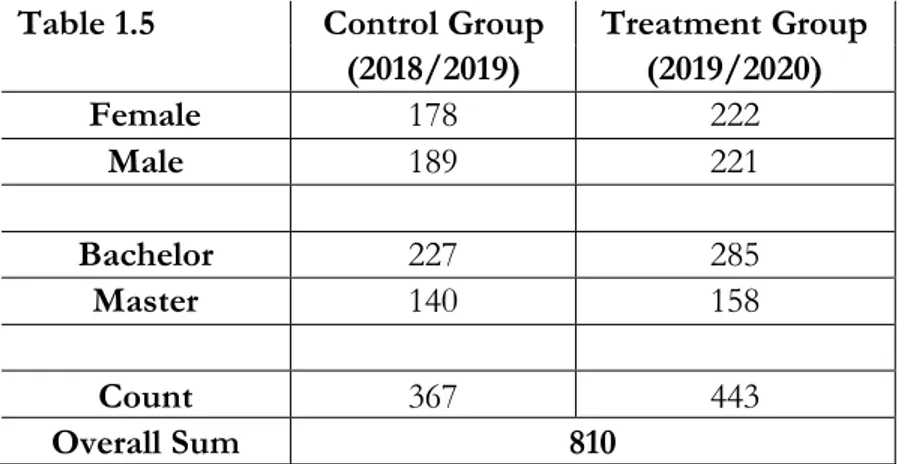
In the following tables (1.5 and 1.6), our descriptive statistics tables are presented. As shown in table 1.5, there were 367 participants in the control group (178 females and 189 males), while the treatment group consisted of 443 participants (222 females and 221 males). There were 512 Bachelor students, out of which 227 belong to our control group, and 298 Master students, out of which 140 belong to our control group. Furthermore, it is interesting to note that, looking at the Table 1.6, our grade difference variable decreases by 0.14 points
on average if the student is in the treatment group. In addition, both the min. and max. value of the grade difference variable is lower in the treatment group.
Table 1.6 Grade Difference Age
Control Group Treatment Group Control + Treatment Group Control Group Treatment Group Control+ Treatment Group Mean -0,35 -0,49 -0.47 24,3 22,7 23.7 Median -0,25 -0,50 -0.50 24 22 23 Std. Dev. 1,23 1,62 1.46 3,5 3,6 3.8 Min -4,50 -4,75 -4.75 19 18 18 Max 3,75 3,50 3.75 41 49 49 5.2 Research Question 1
The first research question investigates if there is a statistically significant difference in the academic performance of students before and after the treatment was implemented, meaning when the classes transferred to digital teaching, due to Covid-19. Our OLS regression results are presented in the following table:
Variable Coefficient Std. Error t-Statistic Prob. C -0.354905 0.076019 -4.668606 0.0000 TR -0.215073 0.102793 -2.092283 0.0367 R-squared 0.005389 Adjusted R-squared 0.004158
Table 1.5 Control Group Treatment Group (2018/2019) (2019/2020) Female 178 222 Male 189 221 Bachelor 227 285 Master 140 158 Count 367 443 Overall Sum 810
Looking at the p-value, we conclude that both the intercept and slope coefficients are statistically significant at 5% level. Thus, we fail to accept the null hypothesis (β1 = 0) and conclude that there is a statistically significant negative effect of the digital semester due to COVID-19 on student academic success. Our estimated model becomes:
𝐺𝐷 = −0.35 − 0.22 𝑇𝑅 + 𝑢 Where the estimated effect coefficients are: 𝐸(𝐺𝐷) = {−0.35 𝑖𝑓 𝑇𝑅 = 0
−0.35 − 0.22 𝑖𝑓 𝑇𝑅 = 1
Thus, the control group grade difference change between the spring 2 and autumn semesters was -0.35 points, while the grade difference change in the treatment group was −0.57. Thus, the effect of the treatment on grade difference between the groups is negative 0.22 points, suggesting worse academic performance of students during the digital semester, imposed due to Covid-19.
5.3 Research Question 2
Our next question to answer is whether there are gender-specific differences in the academic performance of our treatment group, meaning if one gender performed superior to the other when the classes transferred to digital teaching. Our OLS regression results are in the following table:
Variable Coefficient Std. Error t-Statistic Prob. C -0.354905 0.075976 -4.671258 0.0000 TR -0.310636 0.123754 -2.510109 0.0123 TR*G 0.191559 0.138306 1.385038 0.1664 R-squared 0.007747 Adjusted R-squared 0.005288
Looking at the p-values in the table, we notice that the intercept and treatment dummy coefficients are statistically significant at a 5% level. However, the interaction term coefficient significance is rejected both at 5% and 10% level. Our estimated model becomes:
𝐺𝐷 = −0.35 − 0.31 𝑇𝑅 + 0.19 𝑇𝑅 ∗ 𝐺 + 𝑢 where the estimated effect coefficients are:
𝐸(𝐺𝐷) = {
−0.35 𝑖𝑓 𝑇𝑅 = 0; 𝐺 = 0,1 −0.35 − 0.31 𝑖𝑓 𝑇𝑅 = 1; 𝐺 = 0 −0.35 − 0.31 + 0.19 𝑖𝑓 𝑇𝑅 = 1; 𝐺 = 1
Our benchmark group in this model are all the male and female students who belong to the control group. The mean grade difference abetween spring 2 and autumn semesters for the control group is equal to −0.35 points, as estimated in our first model. The differential effect of our interaction term is reported to have a positive effect on the grade difference of 0.19 points if a student in the treatment group is male; however, it is statistically insignificant. Thus, we fail to reject the null hypothesis, and conclude that gender-specific differences do not affect the academic performance of our treatment group. However, the slope coefficient estimating the differential effect of a female student in the treatment group reported to be significant at a 5% level. This suggests that female students in the treatment group performed worse during the digital semester, estimating the effect on their grade difference to be 0.31 points lower when compared to the control group.
5.4 Research Question 3
Our third model investigates group-specific differences in the academic performance of our treatment group when it comes to the educational level. More specifically, it assesses if Bachelor or Master students in the treatment group performed superior to the other when the classes transferred to digital teaching. Our OLS regression results are presented in the following table:
Variable Coefficient Std. Error t-Statistic Prob. C -0.354905 0.074187 -4.783891 0.0000 TR 0.108413 0.112210 0.966165 0.3343 TR*EL -0.906990 0.140966 -6.434104 0.0000 R-squared 0.053921 Adjusted R-squared 0.051576
Looking at the p-values in the table, we notice that the differential effects of the intercept and interaction dummy coefficients are highly statistically significant at a 5% level. In addition, the significance of the differential effect coefficient of Bachelor Students in the treatment group is rejected both at 5% and 10% level. Our estimated model becomes:
where the estimated effect coefficients are:
𝐸(𝐺𝐷) = {
−0.35 𝑖𝑓 𝑇𝑅 = 0; 𝐸𝐿 = 0,1 −0.35 + 0.11 𝑖𝑓 𝑇𝑅 = 1; 𝐸𝐿 = 0 −0.35 + 0.11 − 0.91 𝑖𝑓 𝑇𝑅 = 1; 𝐸𝐿 = 1
Our benchmark group in this model includes all Bachelor and Master students who belong to the control group. The mean grade difference between spring 2 and autumn semesters for the control group equals to −0.35 points, as estimated in our previous two models. The slope coefficient estimating the differential effect of Bachelor students in the treatment group is reported to have a positive effect on grade difference of 0.11 points, which suggests that Bachelor students performed better during the digital semester, compared to the control group; however, it is statistically insignificant, both at 5% and 10% level. Furthermore, the slope coefficient estimating the differential effect between Bachelor and Master students in the treatment group reported to be highly significant at a 5% level. Thus, we strongly reject the null hypothesis (𝛽2 = 0) and conclude that there is a strong negative differential effect of 0.91 points on the academic performance when comparing Master to Bachelor students in our treatment group. More specifically, the effect suggests that Master students performed worse during the digital semester, than Bachelor students did.
5.5 Interpretation of R2
In all three of our models, R2, which is used to examine the goodness of the model fit,
reported being very low, as expected. This can be explained by many different factors that might describe the variability of the regressand, such as the motivation of students, self-discipline, year-specific changes, and others, which stayed unaccounted for.
Furthermore, for the regression results reported in our third model, R2 increased around
10 times compared to model 1 and around 7 times compared to model 2; moreover, our coefficient for the treatment becomes insignificant. This can be a sign of multicollinearity, despite the VIF table results in the appendix indicating no severe multicollinearity in the third model. Usually, this problem can be fixed by either excluding one of the explanatory variables or by including more data. In our case, this cannot be done. Besides reducing the power of the model to identify statistically significant variables, multicollinearity might make it harder to interpret the coefficients. However, if the multicollinearity is only moderate in the model, as in our case, it might not represent an issue.
6 Discussion and Limitations
Even though the results of studies mentioned in our literature review are mixed, they lean towards face-to-face students performing significantly better than online students. This is consistent with our result, in which we found an effect of the treatment on grade difference between the groups being negative 0.22 points, suggesting worse performance during the digital semester, imposed by the Covid-19 outbreak. However, our results contradict the ones found by Gonzalez, et al. (2020) which concluded that the Covid-19 outbreak had a significant positive effect on student performance. Furthermore, it also contradicts the working paper by Loton, Parker, Stein, & Gauci (2020) which claimed a small increase in grades of students, as well as a successful initial transition to remote learning. In studies, where online students did perform better (or worse) compared to face-to-face students, time spent studying, effort and self-discipline was the crucial factor determining success or failure (Anstine & Skidmore(2005); Brown & Liedholm (2002); Calafiore & Damianov (2011); Damianov, o.a., (2009); Navarro (2000); Tseng & Chu, (2010)). In our case, the switch to online studies happened abruptly and during a time when the weather was getting better which might have made it challenging for students to self-discipline and, thus, succeed in online studies. As Navarro (2000) mentioned, many students find it easier to generate motivation and self-direction through a web of student-to-student and professor-to-student interactions.
However, this may not be true for everyone, as there are many unobservable student characteristics, which some researchers (Coates et. al. (2004); Anstine & Skidmore (2005)) tried to account for to avoid sample selection bias in studies where students had a choice between online and traditional courses. These include students’ ability to learn individually, technological skills, and the ability to work with and learn from others.
As Anstine & Skidmore (2005) mentioned, without interactions with peers and lecturers, online students must put in substantially more effort to succeed, which implies that some students simply have the (intrinsic) motivation to succeed regardless of the setting, while others are unable to find the drive to study individually. Besides time spent studying, the GPA was another factor often mentioned as determining online students’ success with higher GPA students being more likely to succeed than those with lower GPAs (Brown & Liedholm (2002); Bennett, Padgham, McCarty, & Carter (2007); Calafiore & Damianov (2011); Damianov et. al. (2009)). In our research, we could not sort out weaker from stronger students based on GPAs, yet we consider this an interesting finding suggesting that weaker
students may have more difficulties learning online. In our case, it may also be that students with extra jobs chose to work more hours, given that traditional lectures were cancelled, which also could have influenced their performance. This may especially be true in cases where no online lectures, or poorly designed online lectures, were perceived as too high of an opportunity cost. While the literature review says (Coates, Humphreys, Kane, & Vachris (2004); Keri (2003)) that bachelor students perform significantly worse compared to master students, our results, with estimates of positive 0.11 points for bachelor students, however insignificant, and minus 0.91 points for master students, suggest the opposite. While the estimate for bachelor students is insignificant, we can still comment on the difference which we believe may be because bachelor students in their first year may have received relatively more support during the transition phase. Master students, on the other hand, might have been perceived to be more independent in comparison and did not receive support to the same extent. Another reason may be overconfidence since master students have been studying courses within their specific fields for a much longer period compared to bachelor students in their first year, they might have overestimated their abilities which reflected their relatively lower performance. The estimated effect of minus 0.31 showed that female students performed significantly worse during the digital semester, compared to male students. This contradicts findings made in (Howsen & Lile, 2008) and (Shoemaker & Navarro, 2000) but is in line with the general research finding that women underperform men in principles of economics courses (Ballard & Johnson (2005); Ziegert (2000); Greene (1997)).
Furthermore, besides the classes being conducted online during the second spring semester of 2020, digital examination was also put in place. This implies that there was no control over the academic integrity and dishonesty during the examination periods which is strictly prohibited by most academic institutions. This could be one of the potential reasons some students in the treatment group performed better compared to students in the control group, which does not necessarily imply higher academic achievement, but rather just an upward trend in the average grades. However, our study found an overall negative effect of the digital semester on student academic performance, meaning that, if academic integrity of students wasn’t satisfied, the effect could have been underestimated.
One limitation of our research, as mentioned in our literature review, are unobservable factors such as the ability to learn individually, technological skills, ability to work with, and learn from others may have had an effect on students’ performance during the digital semester. In other words, given abilities differ from individual to individual, some