I
The Distribution of
Foreigners and Locals in
Sweden.
BACHELOR THESIS WITHIN: Economics NUMBER OF CREDITS: 15
PROGRAMME OF STUDY: International Economics
AUTHOR: Davide Dutto and Duyun Lei JÖNKÖPING December 2019
II
Bachelor Thesis in Economics
Title: Distribution of foreigners and locals in Sweden. Authors: Davide Dutto and Duyun Lei
Tutor: Michael Olsson Date: 2019-12-09
Key terms: Agglomeration, Zipf’s law, Rank size distribution, Migration, Population
Abstract
This study aims to find a relationship between the distribution of locals inside of Sweden and the municipalities’ relative concentration of foreigners. With the usage of data found in the website Statistics Sweden, we aim to investigate the existence of any relationship between the local population size of a municipality against the number of foreigners present in said municipalities, and see whether foreigners and immigrants are more concentrated in more populated municipalities rather than less populated ones. We aim to do this by utilizing multiple regression and dummy variables to identify whether there is a significant extra negative or positive effect on foreigners. The answer seems to be that foreigners are in fact more concentrated in more locally populated municipalities, rather than less populated ones.
III
Table of Contents
1. Introduction ... 1
2. Theory and Literature Review ... 4
2.1 Agglomerations ... 4
2.2 Positive externalities ... 5
2.5 Monocentric city model ... 7
2.6 Migration ... 8 2.7 Sweden Population ... 9 2.8 Hypothesis ... 10
3. Data ... 11
4. Method ... 13
5. Results ... 14
6. Discussion ... 16
7. Future studies ... 17
8. Conclusion ... 19
References ... 21
Appendix ... 24
1
1. Introduction
As time progresses, the phenomenon of immigration and emigration is becoming an increasingly severe issue both on a national and international level. In 2019, there were 272 million international migrations worldwide. This number is 3.5 percent of the share of the global population. This movement occurred mainly between countries. The largest number of immigrants in the world lies within the United States of America (51 million people), equal to about nineteen percent of the world’s total immigrant amount. Germany and Saudi Arabia host the second and third largest numbers of migrants worldwide (around 13 million each), followed by the Russian Federation (12 million), the United Kingdom of Great Britain and Northern Ireland (10 million), and the United Arab Emirates (9 million). Of the twenty main destination countries of international migrants worldwide, seven were in Europe, four in Northern Africa and Western Asia, three in Central and Southern Asia, two in Eastern and South-Eastern Asia, two in Northern America, and one in both sub-Saharan Africa and Oceania (International Migration, 2019).
According to the Cambridge English Dictionary, the definition of migration is the process of animals traveling to a different place, usually when the season changes. When it comes to people, migration becomes an umbrella term, not defined under international law. It typically describes a person who crosses an international border, seeking to either temporarily or permanently relocate, and has left his or her usual residence. These people usually include political refugees as well as people who seek better economic well-being. In this research, we noticed that a common trend of migrants seems to be political refugees from the violence in their countries. There were also other reasons, such as study, work requirements, environmental factors, and so on.
Policies have been implemented and have changed as time went on. For example, Sweden has made new rulings which had the result of increasing the leniency of family reunification in Sweden (The Local, 2018).
2
1.1 Background and aim
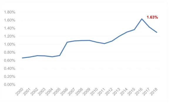
During the middle ages, the largest immigrant groups were merchant trading organizations. Before refugees escaped from their countries due to World War II, Sweden had been a country prone to immigration for a long time. A record-breaking immigration peak has posed a refugee challenge to the country in 2015, which occupied 1.63 percent (Figure 1) of the total population. Stockholm is the largest city and also the capital of Sweden. It happens to also be the largest immigrant cluster space in Sweden, containing about 63 percent of the total immigrants in the country. Migration clusters occurred in Sweden as well as Germany due to welcoming policies that guaranteed a better lifestyle to people in asylum. Syrians are the largest group as share of immigrants, which along with Afghans and others who reached Europe, chose Sweden as their primary destination.
Source: Scb.se
Figure 1- Immigration percentage of the total population in Sweden from 2000 to 2018
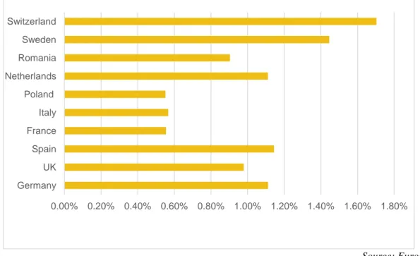
Figure 2 shows the proportion of immigrants in the ten top European countries in 2017, all the countries ordered by population size (Germany is the largest). As we can see, although Sweden has a low position in the rank of the population (ninth), the percentage of immigrants is very high compared to other European countries (second). While it may seem that countries prone to immigration like Sweden only attract people over, based on Statistics Sweden, the country has had a stable number of emigrants (table 8.1,
0.00% 0.20% 0.40% 0.60% 0.80% 1.00% 1.20% 1.40% 1.60% 1.80%
3
appendix) as well. Furthermore, local newspapers used “a record emigrating from Sweden” to describe a large number of emigrants in 2015 (The Local, 2016). The numbers of emigrants in said year doubled those of thirty years prior.
Source: Eurostat
Figure 2- Proportion of immigrants in the total population by European countries in 2017
The research question that is going to be answered during this study is whether foreigners tend to cluster where the local population is highest. To answer this question, we will analyze the location and size distribution of immigration scattered in all the different municipalities of Sweden, giving possible explanations for their locations and what determines their size. We will gather data that indicates the number of foreigners and locals per municipality. After that, compare it to the rank-size distribution model with Swedish population data to investigate whether it is the bigger cities that have more immigrants rather than smaller cities and compare the concentration of foreigners and locals.
1.2 Outline of the thesis
Section two provides a brief literature review as well as theories like agglomeration, externalities, and Rank Size Distribution. In section three, we introduce the data we used to analyze foreigners and locals on rank-size distribution and Zip’s law. Section four shows the method we utilized to achieve a result and give a final answer. Section
0.00% 0.20% 0.40% 0.60% 0.80% 1.00% 1.20% 1.40% 1.60% 1.80% Germany UK Spain France Italy Poland Netherlands Romania Sweden Switzerland
4
five presents the results of our multiple regression, and our final observations on just the data set acquired. Section six focuses on the discussion of the results that we achieve through our regressions, and in section seven, we will give suggestions for future studies that we have not undergone in our paper. Lastly, in section eight, we conclude the whole thesis while giving out some personal considerations.
2. Theory and Literature Review
To fully understand why migrants cluster in space, we need to highlight the concept of agglomeration and its benefits and downfalls. To do so, we need to emphasize the existence of positive as well as negative externalities. Furthermore, to identify how we are going to analyze the societal issue of immigration, Zipf´s law is going to be explained.
2.1 Agglomerations
Agglomerations are a direct result of urbanization. As more cities technologically and economically advance, nuclei of people start to form around critical parts of countries that benefit further economic growth as well as societal welfare. To learn why people cluster in space, we need to consider different factors that entice people to group together. The reasons can be sociological, psychological, historical, cultural, geographical, and economical (Brakman, Garretsen, Van Marrewijk; 2009). Sociological from the point of view that people like to interact and are therefore incentivized to move or stay in places where social interaction is more common. Psychological is a factor due to human nature’s desire for us to be with people rather than being alone. Historical because of the willingness of people to stay in places where relatives have lived prior. Cultural because people enjoy staying around likeminded people. Geographical because some spots can be both objectively and subjectively better than others to live in. Finally, economical – some places provide better economic activities than others, leading to people clustering and creating agglomeration economies. Benefits from economic agglomerations amount to lower transport costs, easier labor mobility, knowledge spillovers due to the clustering of firms (either localization externalities, or urbanization externalities) as well as the inevitable presence of competition, and economies of scale due to lower transport costs and inevitable
5
higher demand because of lower prices on goods, both because of the cheaper cost to create the products as well as the lower price caused by competition (Rigby, Mark Brown; 2013).
2.2 Positive externalities
Externalities are also referred to as spillover effects. Positive externalities are an indirect positive result of something happening. In the case of agglomerations, externalities are a form of knowledge spillover from firms, even of different types. And to some other experts, it can also be a result of competition between two firms that offer the same product/service or internalization of monopoly power. The first concept originates from Jacobs (1969), which states that firms of different industries located in the same geographical area cause positive externalities in the form of knowledge spillovers originating from workers that have different diverse skillsets. The second concept comes from Porter (1990), who states that it is competition between same-type firms which enhances externalities because of the continued pressure to compete against one another. The last concept originates from a thought from Marshall, which instead suggests that monopolies allow for the individual firms to elaborate on their product and/or service and create the best result possible: internalizing the monopoly externality causes an increasingly better product (Carlino, 2001).
2.3 Negative Externalities
Negative externalities, also called de-agglomerating forces, incentivize the de-clustering of people from said agglomerated spaces. These can range from simple pollution due to the large utilization of vehicles in a confined space, or maybe just the lowered appeal of living in the city and upward trend of living in nature and therefore far away from an agglomerated space. As more people are getting conscious about the environment, it might begin to be a positive part of their utility to move away from the city center and into more nature-friendly areas.
2.4 Rank-Size Distribution Model/Rule
The rank-size distribution modeled in the following way. First, all the cities are ordered by their population. The higher the population, the higher the rank (so one is the highest rank) given to the respective city. This value is then plotted against the population of
6
each separate city. As a result, most distributions cataloged this way seem to have a power-law distribution, which indicates a more visible gap between the quantities displayed between the top two ranks, than between all the ranks that follow. This is illustrated as an example in figure three.
Figure 3- Example of a rank size distribution model
The Rank-Size Rule is used as a statistical metric in both developed and underdeveloped countries when the cumulative frequency of cities with a population of greater than twenty thousand people is ranked against the size of a city on a log-normal scale (Planning Tank, 2017). The following formula is used in rank-size distribution:
Where is the population of city , is the constant, and is the rank of the city (municipalities in this case) . This is because the original formula would be:
0 0.2 0.4 0.6 0.8 1 1.2 0 5 10 15 20 25 P op ul ati on v al ue s Rank values
7
Zip’s law holds when the value for q is 1. To note is that the sign used in the logarithmic equation is positive but will turn negative as the gradient of q is negative. The line is then tested against the real values by identifying the value of , which is known as the goodness of fit. When the number is closer to one, the more there is a one to one relationship between the expected population size and real and observed population size. Furthermore, if the value of q (the value that determines how close the real value is equal to Zipf’s expected value for city sizes) is equal to 1, the distribution of immigration in Sweden follows the rank-size rule as well as Zipf’s law. Which means the largest city is (one, two, three…) times larger than the (first, second, third…) city, respectively. If q is smaller than one, a more even distribution of immigration size than Zipf’s law is present. If q is bigger than 1, a more uneven distribution of immigration size than Zipf’s law is represented on the graph.
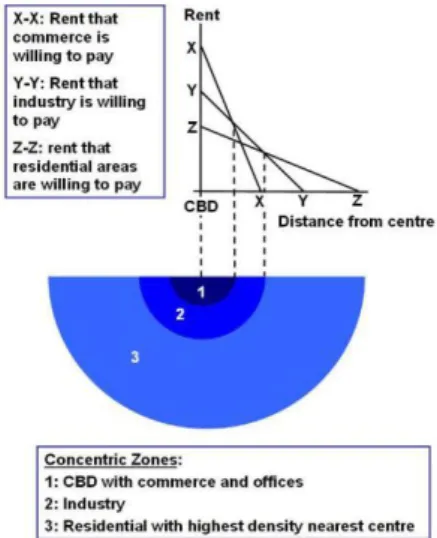
2.5 Monocentric city model
When it comes to the monocentric city model, the first thing that needs to be explained is the bid-rent theory. Bid-rent theory is a geographical economics theory that explains how the demand and hence, the price for land changes with distance from the central business district (CBD) (Von, 1826). Its basic development occurred in the 1960s and 1970s, mainly through the work of William Alonso, Edwin Mills, and Richard Muth. (Alonso, 1964, Mills, 1972 & Muth, 1969). Since that time, cities have become increasingly polycentric, and the monocentric city model, with its assumption of a single concentration of employment, has been criticized on the grounds that the cities it explains are from a different era (Kraus, 2006).
8
The monocentric city model is a descriptive model, which is based on the condition of a featureless plane, perfectly flat and homogenous. The model assumes that commuters live outside the CBD and travel back and forth to their work at the CBD. Each commuter derives utility from his or her space of living but also faces transportation costs. However, they would have higher rent if they wanted to live closer. Hence, there is a trade-off between short distance and cheap housing. Competition for land between commuters implies an efficient allocation of land. Another typical theory about the compromise is the central place theory, which claims that different points or locations on the economic landscape have different levels of centrality and the goods and services efficiently provided on a hierarchical basis (Mulligan, 1984). Hence, it accounts for the distribution of economic activity across space. The situation is similar when it comes to migration, higher utility drives people to move from one place to another.
Utility is defined as the “Satisfaction derived from consumption activities” (McDowell, Thom, Frank, & Bernanke, 2012). This means that people move to another country due to incentives or benefits to the individual. People want to maximize their utility as per its definition, and therefore always look for better lifestyle choices. In microeconomics, this is typically achieved by calculating the most amount of marginal utility one produces by the expenditure of one unit of currency. The good that is bought with the most marginal utility per currency is the good that is purchased to maximize utility. Having said so, this also applies to people that want to lead a better life and choose to move countries to make their living conditions more favorable. Instead of purchasing goods that have the most marginal utility, they instead move to places that cause the same result.
2.6 Migration
The number of migrants has reached two-hundred and seventy-two million in 2019 and is still increasing in an upward trend everywhere in the world. The top three countries with most migrants are the United States of America, Germany, and Saudi Arabia. Migration occurs from people who are just looking for a more beneficial economic situation elsewhere where they think the job market might accommodate them accordingly. A similar movement happens between countries as well, with people seeking opportunities to work for an appropriate higher wage. The following reasons are the cause of most migrations: human-made environmental disasters that make it unsafe to stay in an area, the loss of industries or
9
employers in an area, a less extreme climate, cultural resources, and job opportunities (Hunter, 2019).
Migration mostly occurs out of third world countries due to the individuals’ necessity. Elspeth Guild found that although international protection and refugees attract a large amount of media attention, the first residence permits only account for one quarter in the EU region. The interesting thing is the member state that presents itself as the most migrant-unfriendly country, the UK, is the one that issues the largest number of first residence permits to third-country nationals. The UK had 567,806 migrants in 2014, compared to 355,418 in Poland, the next most liberal issuer of first residence permits. However, the data changed in 2019, providing statistics that differed significantly from those gathered in 2016. In 2016, the UK became the 5th largest migration country in the world and third in the EU. There are many reasons, but one of them could be Brexit (British exit - refers to the UK leaving the EU).
About 3.5 percent of the world population were international migrants, compared to 2.8 percent in the year 2000 (United Nations, 2019). After the war in Syria started, a significant number of Syrians came to EU countries. The Swedish refugee quota increased from 1,900 to 5,000 places since 2016. Sweden is now the third-largest recipient country when it comes to taking in migrants (Swedish Migration Agency, 2018). Fredrik Bengtsson, says: “The year 2014 was the second-highest level on record for asylum-seeking applications; second only to 1992 when more than 84,000 people, many of them fleeing the former Yugoslavia, requested asylum in Sweden.” After the migration reached a peak in 2015, the government had to take some measures (changes in Swedish migration laws) to limit immigration, to be able to provide for those already in the country. In 2019, Sweden still had 2,005,200 international migrants, which included 14.6 percent of refugees. The proportion of refugees is enormous since the share of refugees is only 4.4 percent in the EU region.
2.7 Sweden Population
In 2019, the population of Sweden reached ten million, becoming the 91st largest country in the world by population. The total land area of Sweden is about 450 000 . The population distribution is very uneven, with 87.9 percent of the population living in urban areas. Sweden is covered by forests, lakes, rivers, and contains thousands of small islands. According to Statistics Sweden (SCB), the population density is about 57.5 people per square mile, with a higher population density in the south than in the north. Stockholm is the capital and largest
10
city in Sweden, with 2.35 million people in the greater metropolitan area, and around one million within the city limits (World Population Review, 2019). The median age of the total population in Sweden is 40.9 years (Worldometers, 2019).
The demographics of Sweden have changed remarkedly since immigration surged after 2012. In 1570, population started to count at 900,000. As we can see in figure 5, the population growth is unstable between 1570 to 1970. After that, there is a stable trend until 2015. The highest growth rate is around 48 percent in the year of 1895 and 1900. The lowest rate is 0.5 percent in 1995. According to SCB, one in five people in Sweden may have a foreign background.
Source: Statistics Sweden
Figure 5- Population Growth Rate
2.8 Hypothesis
After doing all the research, we expect to have some form of relationship between the size in population of Swedish municipalities and their respective sizes of foreign citizens living there. This is because of how Statistics Sweden defined the concept of immigrants and foreign citizens. It would not make sense for a city such as Stockholm to not contain the most amount of foreign people. Stockholm is a place of interest for many kinds of people, whether they want to work there or study there. In our opinion, the inevitable result will be a statistical significance between local population spread and foreign population spread within the different municipalities in Sweden, while also having an uneven cluster of foreigners concentrated in the most populated cities. We think that the result of the multiple regression
0.00% 10.00% 20.00% 30.00% 40.00% 50.00% 60.00% 1570 1650 1700 1750 1800 1850 1900 1950 1970 1980 1990 1995 2000 2005 2010 2015
11
will statistically show that locals will live more spread out in the country than foreigners do, with foreigners more concentrated around the most populated parts of Sweden.
3. Data
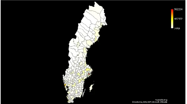
Before delving into the data part of the study, we believe it to be appropriate to show a heatmap of the concentration of the population of Sweden
Figure 6- Heatmap of total population in Sweden
12 0 200000 400000 600000 800000 1000000 1200000
To begin with, we will point out that all the data that we used for immigrants are actually for foreigners. It was challenging to find a data set that only included immigrants. For one, it was hard to find data for immigrants that was not a single immigration action (coming in the country). For two, immigrants do not include a wide variety of individuals who come into the country for similar reasons as immigrants but not included in the immigration listings (students).
We specifically looked at the top twenty municipalities to get an interesting result of the municipality data — these graphs created with the number of each population on the y-axis and ranks on the x-axis. Having so many municipalities with such a relatively low amount of people in the entirety of Sweden seems to cause a shape of the likes of the one portrayed in our expected result of the population that we talked about in the literature section (power-law distribution). We then decided to remove the smallest municipalities and only see a graphical depiction of the size of the top twenty biggest municipalities, from which we can draw more interesting results.
Table 1- Descriptive Statistics for Foreign and Total
Foreign Total Min 9731 97381 Max 110068 962154 Count 20 20 Standard Deviation 25099.76405 210276.2859 Mean 16719.94061 158192.8 Median 12846 133171
13 0 20000 40000 60000 80000 100000 120000
Figure 9- Population of foreigners in top twenty municipalities in Sweden ordered by rank
We can notice that Stockholm, Göteborg, Malmo and Uppsala are the top four municipalities in both criteria. This leads us to believe that the size of the city is a contributing factor to foreigners. The data we acquired probably includes students, also providing another reason as to why this might be. Stockholm and Göteborg, cities/counties renowned for their level of provided education, attract many foreigners willing to study in Sweden. This can be a contributing factor to a similar trend in the distribution of both categories. Also, the order in which the different municipalities are respective to their categories is interesting. Most cities in the first graph are also in the second, albeit in a different order, possibly another reinforcement for our earlier assumptions.
4. Method
To begin with, we created a data set that was created by removing the foreign population from the total population to create a new data set that exclusively held the local population between municipalities. Furthermore, the process is to create a simple regression of the two data sets by putting the natural logarithm of the rank on the x-axis and the natural logarithm of the population amount on the y-axis. The theory behind this is discussed in the theory section underneath part two of this thesis. This allowed us to view the simple regression for both local and foreign exclusive from one another on the same graph. However, this was not the way that we tested for the presence of Zipf’s law or population concentration between different municipalities.
14
To test whether there would be a difference between the spread of the local population and the foreign population, we used multiple regression using dummy variables. We gave the dummy variable relating to the foreign population a value of one. Likewise, we gave the dummy variable of zero to the data that was part of the local population. The formula used is
This is the logarithm of the formula
We theorize that the value for will be positive. This is because that would be the intercept for the value of the local population. As a result, is expected to be negative, since the intercept for the foreign population should be lower due to less foreigners than locals in the top-ranking municipality. We also expect and to be negative. This is because the slope of the two simple linear regressions should be negative, as the logarithm of the rank should increase as the logarithm of the population decreases. Once we get the result, we will investigate whether another country yields similar results. We will test for Norway to either further reinforce our results or to dispute them.
5. Results
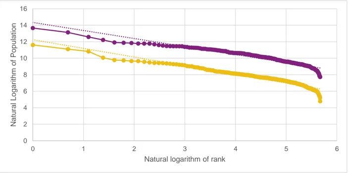
Let’ s set up a multiple regression using data for local and foreign population. First, we remove the foreign population from the total population data. We then put them on the same graph while having the logarithm of the rank on the x-axis, and the logarithm of the population on the y-axis.
15
Figure 10- Local vs Foreign spread of population (Purple vs Yellow respectively). Purple = Local, Yellow = Foreign
We then create dummy variables to indicate whether the data comes from the foreign data set or the local data set. We gave the values coming from the foreign data set a dummy variable of one, zero otherwise.
Table 2- Summary Output
Regression Statistics Multiple R 0.9847 R Square 0.9696 Adjusted R Square 0.9694 Standard Error 0.2790 Observations 580 ANOVA df SS MS F Significance F Regression 3 1427.3163 475.7721 6113.5107 0.0000 Residual 576 44.8261 0.00778 Total 579 1472.1424 Coefficients Standard Error t stat P-Value Lower 95% Upper 95% Lower 95.0% Upper 95.0% Intercept 14.3346 0.0813 176.268 0.000 14.175 14.494 14.175 14.494 Logr -0.972 0.017 -57.167 0.000 -1.006 -0.939 -1.006 -0.939 D -2.087 0.115 -18.148 0.000 -2.313 -1.861 -2.313 -1.861 DlogR -0.079 0.024 -3.287 0.001 -0.126 -0.032 -0.126 -0.032 0 2 4 6 8 10 12 14 16 0 1 2 3 4 5 6 Natu ral Lo ga ri thm of P op ul ati on
16
We get the P-value of 0.001 for Because this is statistically significant, we agree that the value of the coefficient of the DlogR is statistically significant. The value of is the extra negative effect on the foreign population. Furthermore, we seem to have been correct on our former assumptions when it comes to the values of the coefficients. We indeed got a value of that is positive, and a value of that is negative. Furthermore, the value for is negative as expected (-0.972), and due to the extra negative effect on foreign population, we get a value of that is -1.051, also negative, albeit even more negative than the value of
.
6. Discussion
Initially, we were of the idea that the foreign population would gather around places with many locals. This is because we theorized that the large appeal for a foreigner to go somewhere is caused by the thriving economic/sociologic environment at its destination. Therefore, it would be reasonable to assume that foreigners would target places with an already big economy and a large population. Much like we saw in the graphs prior, Stockholm and Goteborg indeed do have the biggest local populations in Sweden, both for local and foreign. We theorized that part of this reason was because of the education provided by the two municipalities. When we look into the multiple regression, it seems that the gradient for the foreign population is steeper than the local population’s due to the extra negative effect on foreigners, indicating that higher-ranked municipalities (so less population) have a lower ratio of foreign to the local population. This would also support the fact that the highest foreign-local ratio would be found in the municipalities with the most amount of people.
What can we then conclude about how distributed the local and foreign populations are throughout the different Swedish municipalities? Looking at the multiple regression, we get values for the gradient of each slope that do not amount to the perfect value that would be 1, indicating a perfect fit of the populations to that of Zipf’s law. Having said so, the gradients for the two linear equations do tell us how evenly distributed the two population spreads are. The fact that the gradient of the local population equation is less than the absolute value of one, and that the gradient of the foreign population is more than the absolute value of one, we can conclude that the populations for each are more evenly spread out than predicted, and less evenly spread out than predicted respectively. This means that foreigners are more
17
agglomerated in places with an already high local population, and less so in places with a low local population.
Is this always the case? We have come to the conclusion that foreigners are more concentrated than expected in the biggest municipalities population-wise when it comes to Sweden. What if we were to try and test another country? By undergoing the same process and taking data from Statistics Norway, we get a multiple regression model with the same dummy variables set up (1 if foreign, 0 if local). The results of this regression can be found in the appendix under table 2.
We mostly get similar results for Norway as the ones we got for Sweden. First of all, we get an extra significant negative effect on foreign population that increases the concentration skew of foreigners towards the bigger populated cities. Second, we can see that is in this case -1.279, indicating that yes, just like Sweden, foreigners are more concentrated to the bigger cities. However, unlike Sweden, it seems that the local population of Norway is also more concentrated in bigger cities with a that is less than -1. Though we cannot conclude that foreigners are always more concentrated in the most populated municipalities of a country, by looking at one of Sweden’s neighbors, we can see a striking resemblance to the pattern of foreign population distribution between the two countries.
7. Future studies
This thesis studied the distribution of foreigners in Sweden and compared it to its locals. In other words, we tested to see which one is more concentrated when it comes to the distribution of foreigners and locals. During the research, we found some limitations and possible improvements to the overarching process. There are still many kinds of tests as well as possible research that we were not able to accomplish due to the existence of a time restriction.
First, migration is a vast and fascinating research subject. We found that there are a lot of reports or datasets, which divided migration into all different categories (different regions, countries, age groups, and so on). We think that there are considerable possibilities to extend our study into a bigger map or narrow down our concentration to individuals. It would be very interesting to analyze results from more countries, (Europe) or choose one country from a
18
different region (America, Asia, Africa, Oceania). Comparing their results will give a more comprehensive understanding of the distribution of migrants and foreigners. When we researched the data that we would need to accomplish this paper, we found a unique dataset about migrants divided by age group. In 2019, there were about 74.2 percent of migrants between twenty to sixty-four years old, and 13.9 percent and 11.9 percent represented by the proportion of migrants who were less than 19 years old and more than 65 years old respectively in the world. Naturally, the adults will have more mobility, energy, and time compared to a child, teenager or elderly. Different countries may have a different outcomes, and it would be interesting to compare them in the form of a further study.
It might be interesting to categorize said foreigners into their state of origin. Whilst we originally attempted to do so, we found incredible difficulty in this sorting because of how loose the definition of an ‘immigrant’ is. Because we did not want to skew our results too much, we decided to take the values for foreigners to count for the entirety of people coming or living in Sweden that were not originating from there. This allowed us to have a more wholistic view of foreign population and clustering, but the usage of control variables that specify location of origin from these individual people might result in an interesting outcome to both assessing and predicting where future immigrations of foreigners might happen around a country/state/city, and where they originate from.
In this paper, we wanted to focus on the reasons why people move and migrate around the world. In the theory and literature review part, we wrote some possible factors but did not extend them or analyze them in depth. By choosing datasets about different factors as variables, we can use panel data regression to explain how those factors can affect migration. An example of this could be Brexit, as it is a considerable factor contributing to the change of migration patterns in the UK. One of the goals of Brexit was to remodel the UK’s immigration system, arguably making immigration in both the UK and EU look very different once the UK leaves the bloc (King and Flynn, 2018). It would be interesting to analyze the changes caused by brexit in future studies.
Another interesting possible study would be to repeat the multiple regression for countries on different income levels. While it might be interesting to see how immigration and foreign concentration works on a scale of two very similar countries, it might be just as interesting to see how impactful GDP would be regarding both immigration influx and foreign
19
concentration. There’s obviously colonized countries like in Africa which would have a large concentration of foreign people relating to the colonized areas of the countries. Nonetheless, it would be interesting to see this statistical data on paper to see how either the GDP or size of the country itself impacts foreign concentration. What about smaller independent countries like Monaco inside of France? Monaco specifically sounds like an interesting case study, for both its renown as being a rich country while also being relatively small. We feel it would most likely have skewed our results dramatically, and therefore would not be an applicable case study for our purposes. However, if one were to pick this study up once more, the study of independent, albeit tiny countries might be interesting in regards to immigration influx and its possible clusterings of people.
A further study would be to pick different scales in terms of geographical area. While we limited ourselves in the confines of municipalities within two countries, it might also be interesting to see how this clustering varies concerning a continent, like the entirety of Europe or America. Having said so, we assume the result would be that the foreign clustering would be around the most populated capitals of each respective country (or state) inside their relative continents.
8. Conclusion
Initially, we hypothesized that there would a statistical significance with a value of the q for foreign being higher than the absolute value of one, indicating that the concentration of foreigners would be more clustered around the most locally populated parts of Sweden. As part of our calculations and results, we saw this relationship, reinforcing that our initial impressions were accurate and that foreigners tend to cluster more in higher densely populated cities. We then went on to ask the question of whether or not this would always be true. We took one of Sweden’s neighbors in the form of Norway to see whether or not this was also the case. To no surprise, we received a similar statistical answer. While we can’t explain why the locals are more unevenly spread out in Norway than in Sweden, we believe that the norm for countries that allow for immigration within their borders have an uneven spread of foreigners concentrated at the core of the country. This said, as pointed out in the future studies section of the paper, the population being more evenly/unevenly spread out than what Zipf’s law would indicate is something that may vary between countries and
20
geographical locations, and is something that might need to be picked up further on in the future by another study. We believe however, that even though the result was somewhat predictable, this study was important in defining what factors might influence immigration, those being of the likes of education, job opportunity, or economic welfare.
As international students, and therefore foreigners ourselves, we can also vouch that the reasons we have moved to where we have were for reasons that would maximize our utility in terms of better education. This is not always the case, as other times, said reasons might have to do with more minor things like the weather, or social interactions. Nonetheless, we doubt that the phenomenon of immigration will ever stop. As the world gets more globally connected, it’s doubtful that people will stop looking for better lifestyles outside of their home country in the hopes that the neighbor’s grass is indeed greener than theirs.
21
References
BBC. (2019, October 29). Brexit: All you need to know about the UK leaving the EU. Retrieved from: https://www.bbc.com/news/uk-politics-32810887
Brakman, S., Garretsen, H., & van Marrewijk, C. (2009). The new introduction to geographical economics. Cambridge University Press.
Carlino, A. (2001). Knowledge Spillovers: Cities’ Role in the New Economy. Business review Q4 2001. Philadelphiafed.org. Retrieved from: https:
//www.philadelphiafed.org/-/media/research-and-data/publications/business-review/2001/q4/brq401gc.pdf
Chappelow, J. (2019). Utility. Retrieved from: https://www.investopedia.com/terms/u/utility.asp
Glaeser, L., Kallal, D., Scheinkman, A., & Shleifer, A. (1992, December). Journal of political economy, Growth in Cities. Vol 100, no. 6, Centennial issue, pp 1126-1152. Published by the university of Chicago press.
Guild, E. (2016, January 22). Rethinking Migration Distribution in the EU: Shall we start with the facts? Retrieved from:
https://www.ceps.eu/system/files/No%2023%20EG%20on%20Migration%20Distribution.pdf
Hunter, N. (2019). Why communities move adapted from Migration: Reasons to move. Retrieved from: https://www.nationalgeographic.org/activity/why-communities-move/
Kraus, M. (2006). Monocentric Cities. Retrieved from: https://doi.org/10.1002/9780470996225.ch6
Man, M., & Ren, M. (2019 May). Wealth Inequality Analysis based on 21 EU countries. Retrieved from: http://www.diva-portal.org/smash/get/diva2:1322552/FULLTEXT01.pdf
22
McDowell, M., Thom, R., Frank R., & Bernanke, B. (2012, March 16). Principles of Economics (European edition). McGraw-Hill
Planning Tank. (2017, January 1). The Rank-Size Rule by George Zipf (1949). Retrieved from: https://planningtank.com/settlement-geography/rank-size-rule-by-george-zipf-1949
Rigby, L.,& Mark, B. (2013, January 29) Who benefits from Agglomeration? Department of geography, University of California – Los Angeles, Los Angeles CA, 90095. Retrieved from: https://www.tandfonline.com/doi/abs/10.1080/00343404.2012.753141
Rütt, B. (2010). Location and rank-size distribution of Arts and Entertainment: A study of US Metropolitan Regions. Retrieved from:
http://www.diva-portal.org/smash/get/diva2:408504/FULLTEXT01.pdf
Soo, K.T. (2004). Zipf’s Law for Cities: A Cross Country Investigation, Regional Science and Urban Economics, 35(3), 239-263. doi: 10.1016/j.regsciurbeco.2004.04.004
Statistics Norway. (2019). Retrieved from: https://www.ssb.no/en
Statistics Sweden. (2019). Retrieved from: https://www.scb.se/en/
Sweden. (2019). Sweden and Migration. Retrieved from: https://sweden.se/migration/#2015
Swedish Migration Agency. (2018, February 20). Sweden is the third largest recipient country of quota refugees. Retrieved from: https://www.migrationsverket.se/English/Startpage.html
The local. (2016, October 12). Record numbers emigrating from Sweden. Retrieved from: https://www.thelocal.se/
23
The local. (2019, June 19). Immigration: Sweden rolls back strict rules on family
reunification. Retrieved from: https://www.thelocal.se/20190619/sweden-rolls-back-strict-rules-on-family-reunification
UNHCR. (2016). ‘Refugees’ and ‘Migrants’ – Frequently Asked Questions (FAQs). Retrieved from: https://refugeesmigrants.un.org/definitions
UN MIGRAION. (2019). Who is a migrant? Retrieved from: https://www.iom.int/who-is-a-migrant
World Population Review. (2019). Sweden Population 2019. Retrieved from: http://worldpopulationreview.com/countries/sweden-population/
24
Appendix
Appendix table 1 - Emigration in Sweden
Appendix table 2- Multiple regression table Norway Regression Statistics Multiple R 0.9657 R Square 0.9326 Adjusted R Square 0.9323 Standard Error 0.4221 Observations 842 ANOVA df SS MS F Significance F Regression 3 2066.0236 688.6745 3863.992 0 Residual 838 149.3557 0.1782 Total 841 2215.3793 Coefficients Standard Error t stat P-Value Lower 95% Upper 95% Lower 95.0% Upper 95.0% Intercept 14.120 0.109 129.616 0.000 13.906 14.334 13.906 14.334 Logr -1.134 0.021 -53.532 0.000 -1.175 -1.092 -1.175 -1.092 D -1.341 0.154 -8.707 0.000 -1.644 -1.039 -1.644 -1.039 DlogR -0.145 0.030 -4.843 0.000 -0.204 -0.086 -0.204 -0.086 45294 39240 48853 51179 51747 50715 51237 55830 45878 45620 46981 0 10000 20000 30000 40000 50000 60000 2008 2009 2010 2011 2012 2013 2014 2015 2016 2017 2018