DISSERTATION
ADJUSTING FOR CAPTURE, RECAPTURE, AND IDENTITY UNCERTAINTY WHEN ESTIMATING DETECTION PROBABILITY FROM CAPTURE-RECAPTURE
SURVEYS
Submitted by Stacy L. Edmondson Department of Statistics
In partial fulfillment of the requirements For the Degree of Doctor of Philosophy
Colorado State University Fort Collins, CO
Summer 2015
Doctoral Committee: Advisor: Geof Givens Jean Opsomer
Piotr Kokoszka Barry Noon
Copyright by Stacy L. Edmondson 2015 All Rights Reserved
ABSTRACT
ADJUSTING FOR CAPTURE, RECAPTURE, AND IDENTITY UNCERTAINTY WHEN ESTIMATING DETECTION PROBABILITY FROM CAPTURE-RECAPTURE
SURVEYS
When applying capture-recapture analysis methods, estimates of detection probability, and hence abundance estimates, can be biased if individuals of a population are not correctly identified (Creel et al., 2003). My research, motivated by the 2010 and 2011 surveys of West-ern Arctic bowhead whales conducted off the shores of Barrow, Alaska, offers two methods for addressing the complex scenario where an individual may be mistaken as another indi-vidual from that population, thus creating erroneous recaptures.
The first method uses a likelihood weighted capture recapture method to account for three sources of uncertainty in the matching process. I illustrate this approach with a detailed application to the whale data.
The second method develops an explicit model for match errors and uses MCMC methods to estimate model parameters. Implementation of this approach must overcome significant hurdles dealing with the enormous number and complexity of potential catch history config-urations when matches are uncertain. The performance of this approach is evaluated using a large set of Monte Carlo simulation tests. Results of these test vary from good perfor-mance to weak perforperfor-mance, depending on factors including detection probability, number of sightings, and error rates. Finally, this model is applied to a portion of the bowhead survey data and found to produce plausible and scientifically informative results as long as the MCMC algorithm is started at a reasonable point in the space of possible catch history configurations.
ACKNOWLEDGEMENTS
This work was supported and funding by the North Slope Borough (Alaska) and the Na-tional Oceanic and Atmospheric Administration (through the Alaska Eskimo Whaling Com-mission). This research also utilized the CSU ISTeC Cray HPC System supported by NSF Grant CNS-0923386
TABLE OF CONTENTS
ABSTRACT . . . ii
ACKNOWLEDGEMENTS . . . iv
LIST OF TABLES . . . x
LIST OF FIGURES . . . xiii
1 INTRODUCTION 1 1.1 Capture Recapture Surveys . . . 1
1.1.1 Uncertain captures and recaptures and the goal of this dissertation . 2 1.2 Whale Dataset . . . 3
1.3 Overview . . . 5
2 WEIGHTED LIKELIHOOD APPROACH 6 2.1 Introduction . . . 6 2.2 Data . . . 8 2.2.1 Linking Sightings . . . 9 2.2.2 Match Data . . . 12 2.2.3 Covariate Data . . . 15 2.2.4 Data Exclusions . . . 18 2.3 Analytical Methods . . . 19 2.3.1 Chain Weighting . . . 19
2.3.2 Group Size Consistency . . . 23
2.3.3 Detection Probability Estimation . . . 27
2.4 Results . . . 35
2.4.1 Main Findings . . . 35
2.4.2 Other Results . . . 37
3 EXPLICIT MODEL FOR UNCERTAINTY ABOUT CAPTURE,
RE-CAPTURE AND ANIMAL IDENTITY 43
3.1 Introduction . . . 43
3.2 Notation and Definitions . . . 44
3.3 Parameters . . . 47
3.3.1 Effective Parameters for Error Rates . . . 49
3.3.2 Effective Parameter for Detection Probability . . . 55
3.4 Data . . . 59
3.5 Likelihood . . . 61
3.6 Estimation Framework . . . 62
3.7 Markov Chain Monte Carlo . . . 65
3.8 Discussion . . . 80
4 MONTE CARLO EVALUATION OF PERFORMANCE 81 4.1 Sampling Procedure . . . 81
4.1.1 Overview . . . 81
4.1.2 First Level of Sampling . . . 82
4.1.3 Second Level of Sampling . . . 83
4.1.4 Third Level of Sampling . . . 84
4.1.5 Summary . . . 84
4.2 Model Performance Results . . . 86
4.2.1 Overview . . . 86
4.2.2 Informative Data . . . 87
4.2.3 Summary Statistics and Visual Graphics . . . 88
4.2.4 Scenario 1 Results . . . 90
4.2.5 Scenario 2 Results . . . 91
4.2.6 Scenario 3 Results . . . 92
4.3 Summary . . . 94
5 BOWHEAD WHALE EXAMPLE 107 5.1 Data . . . 107
5.2 Analysis . . . 110
5.3 Results . . . 110
5.4 Sensitivity Analysis for Configurations . . . 115
5.4.1 Results for The First Extreme Configuration . . . 115
5.4.2 Results for the Second Extreme Configuration . . . 116
5.4.3 Sensitivity Analysis for Realistic Configurations . . . 123
5.4.4 Discussion of Sensitivity Analysis Results for Configurations . . . 127
5.5 Sensitivity Analysis for the Effective Parameters . . . 127
5.5.1 Results Sensitivity Analysis for the Effective Parameters . . . 128
5.5.2 Discussion of Sensitivity Analysis Results for Effective Parameters . . 128
6 CONCLUSION 133 6.1 Review . . . 133
LIST OF TABLES
2.1 Link codes for sightings of whales or groups. Every sighting is classified with one of these codes. The three fundamental classifications are New, Duplicate,
and Conditional. . . 10
2.2 Main covariates recorded or derived from sightings data in addition to the time, location, and link code. . . 18
2.3 Possible alternative configurations and probabilities for the match chain N1 A ⇔ N2 G ⇔ C1 where the letters above the match arrows indicate match quality ratings. The original chain is most likely and is listed first. . . 23
2.4 Detection probability estimates using the Decon↓ method for the simple and complex models from analysis of the 2011 survey data. The top portion of the table shows sample-weighted means of detection probability estimates from each model, and the mean that would be obtained if the parameter esti-mates from our preferred simple model were applied to the non-deconstructed dataset. Predictions for single whales and groups at several distances are also shown in the bottom half of the table. These estimates are also based on the simple model and Decon ↓. . . 35
2.5 Sample-weighted mean estimated detection probabilities for the three methods of addressing (or ignoring) group size inconsistency. Results are shown for both fitted models (simple and complex). . . 37
2.6 Results of sensitivity analysis using high, medium, and low match confidence weights with the Decon↑ method for addressing group size inconsistency. Al-though Decon↑ is not our recommended approach, it is used here because it produces intermediate results with the medium weights in Table 2.5. . . 40
3.1 Configurations in E1 for Example 3.1 . . . 46
3.2 Configurations in E2 for Example 3.1 . . . 47
3.4 Reduced space of outcomes for Example 3.2. . . 50
3.5 Unrestricted space of outcome probabilities for Example 3.2. . . 54
3.6 Restricted space of outcome probabilities for Example 3.2. . . 54
3.7 Unrestricted space of duplicate sighting outcomes for Example 3.3. . . 56
3.8 Restricted space of duplicate sighting outcomes for Example 3.3. . . 56
3.9 Probabilities for the outcomes in the unrestricted space for Example 3.3. . . 58
3.10 Probabilities for the outcomes in the restricted space for Example 3.3. . . 59
3.11 Match/Non-Match data, Y1,1, for interval 1 and replicate 1 (Rep 1) for Exam-ple 3.4. . . 60
3.12 Match/Non-Match data, Y1, for interval 1 and replicates 1-3 (Rep 1, Rep 2 and Rep 3 respectively) for Example 3.4. . . 60
3.13 Match/Non-Match data, Y , for intervals 1 and 2 and replicates 1-3 (Rep 1, Rep 2 and Rep 3 respectively) for Example 3.4. . . 60
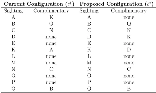
3.14 Current configuration, et1. . . 68
3.15 Current configuration, et1, and proposed configuration, e∗, with sw1=A and sw2=K. . . 69
3.16 Current configuration, et 1, and proposed configuration, e ∗, with s w1=A and sw2=N. . . 70
3.17 Current configuration, et 1, and proposed configuration, e ∗, with s w1=D and sw2=K. . . 71
3.18 Current configuration, et1, and proposed configuration, e∗, with sw1=D and sw2=M. . . 72
4.1 w1,1 and w2,1 pairs chosen for each scenario. . . 85
4.2 Typical true values of ˜αs, ˜αd, ˜β for the 8 cases. . . 86
4.3 95% Coverage Rates of 95% credible intervals for ˜αs, ˜αd, ˜β and ˜p for the 8 cases in scenario 1. . . 89
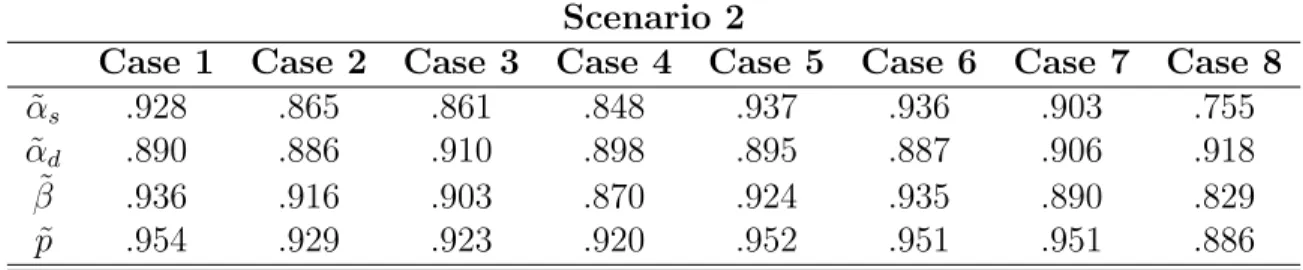
4.4 95% Coverage Rates of 95% credible intervals for ˜αs, ˜αd, ˜β and ˜p for the 8
cases in scenario 2. . . 89
4.5 95% Coverage Rates of 95% credible intervals for ˜αs, ˜αd, ˜β and ˜p for the 8 cases in scenario 3. . . 90
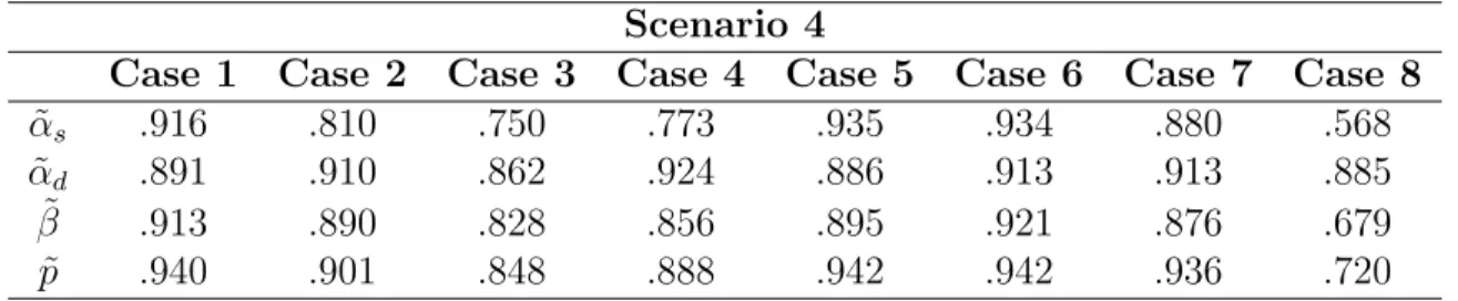
4.6 95% Coverage Rates of 95% credible intervals for ˜αs, ˜αd, ˜β and ˜p for the 8 cases in scenario 4. . . 90
5.1 Bowhead Data; 4/8/10; 14:15-16:45; Perch 1. . . 108
5.2 Bowhead Data; 4/8/10; 14:15-16:45; Perch 2. . . 109
5.3 Posterior distribution summary statistics. . . 112
5.4 Posterior distribution summary statistics when using Rep 1, Rep 2 and Rep 3 as initial configuration. . . 123
5.5 Initial starting values for the three combinations. . . 127
5.6 Posterior distribution summary statistics for the lower extreme, upper extreme and mid range initial starting values for each effective parameter. . . 128
LIST OF FIGURES
2.1 Example of the software display for matching sightings during about two hours on May 8, 2010. Sightings (dots) are labeled by link code and time, and associated by perch according to dot shade. Links and matches are indicated by line segments of different shades. The software displays data but does not attempt any automatic matching. . . 11 2.2 Separation of paired matched sightings in space and time. Each dot represents
a match pair. The data have been transformed by taking square roots to better separate the dots. The E/G/A categories are explained in Section 2.2.2. E matches (black dots) are the most certain, G matches (plus symbols) are intermediate, and A (open circles)matches are the least certain. . . 12 2.3 Example match chain structure from 2010. Sightings are ordered in time
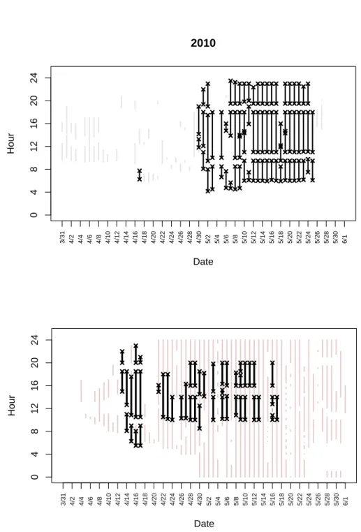
(flowing from left to right). The vertical axis is irrelevant except to separate the two perches. Arcs represent links and arrows are matches. The sight-ing notation (N/C/X/Z) is explained in Section 2.2.1; the match notation (E/G/A) is explained in Section 2.2.2. . . 16 2.4 IO effort for 2010 and 2011 survey years. Each vertical line represents one
day. Black lines represent time with 2-perch IO effort. The boundaries of these periods are indicated with an ‘x’. Gray lines indicate periods when only one perch was used. . . 41 4.1 Plot of probabilities of w1,1 and w2,1 pairs (circle areas) for scenario 1. The
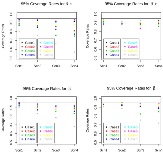
five pairs of values examined in my trials correspond to the red triangles. . . 95 4.2 Coverage rates for 95% credible intervals for each case for ˜αs, ˜αd, ˜β, and ˜p. . 96
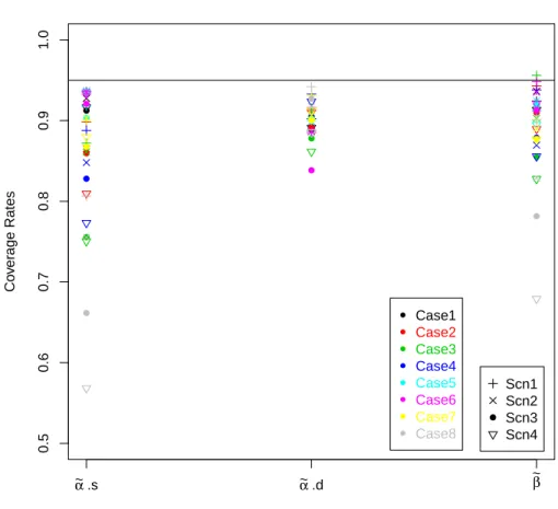
4.3 Coverage rates for 95% credible intervals for each parameter, ˜αs, ˜αd, and ˜β. . 97
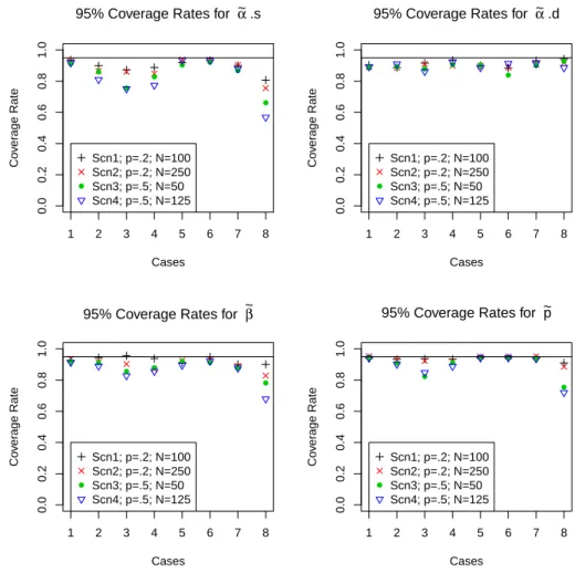
4.4 Coverage rates for 95% credible intervals for each scenario for ˜αs, ˜αd, ˜β, and ˜p. 98
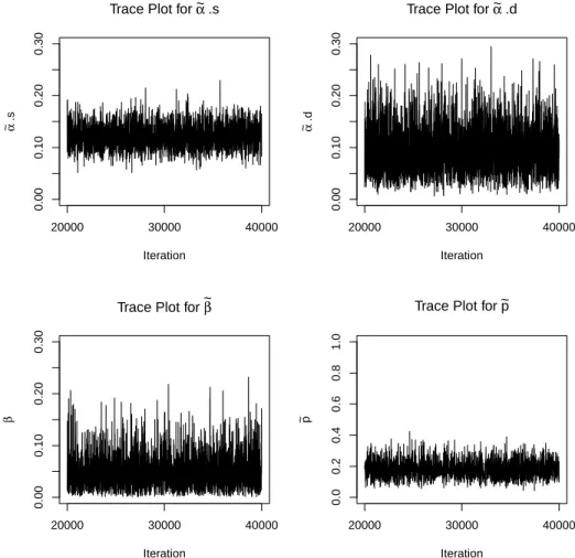
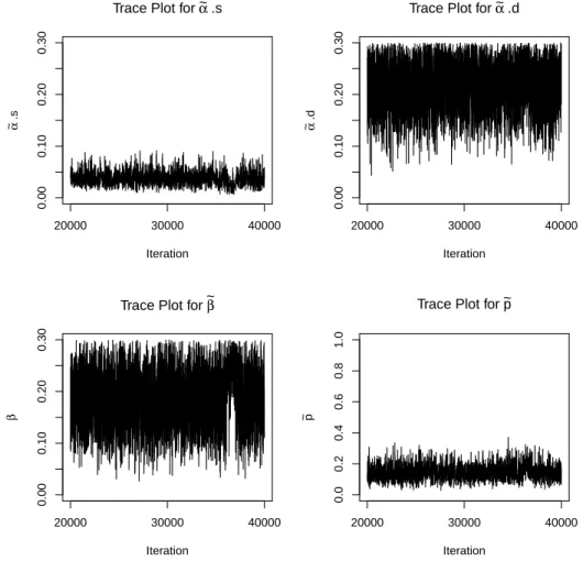
4.5 Trace plots for a simulated data set in scenario 1 case 1. . . 99 4.6 Trace plots for a simulated data set in scenario 1 case 8. . . 100
4.7 Trace plots for a simulated data set in scenario 2 case 1. . . 101
4.8 Trace plots for a simulated data set in scenario 2 case 8. . . 102
4.9 Trace plots for a simulated data set in scenario 3 case 1. . . 103
4.10 Trace plots for a simulated data set in scenario 3 case 8. . . 104
4.11 Trace plots for a simulated data set in scenario 4 case 1. . . 105
4.12 Trace plots for a simulated data set in scenario 4 case 8. . . 106
5.1 Trace plots for ˜αs, ˜αd, ˜β, and ˜p. . . 112
5.2 Histograms for posterior samples for ˜αs, ˜αd, ˜β, and ˜p. . . 113
5.3 Autocorrelation plots for MCMC simulations for ˜αs, ˜αd, ˜β, and ˜p. . . 114
5.4 Trace plots for ˜αs, ˜αd, ˜β, and ˜p for extreme case 1; 40,000 iterations, burn-in 20,000. . . 117
5.5 Histograms for ˜αs, ˜αd, ˜β, and ˜p for extreme case 1; 40,000 iterations, burn-in 20,000. . . 118
5.6 QQ plot comparing the results from the original analysis and the first extreme configuration analysis for each parameter. . . 119
5.7 Trace plots for ˜αs, ˜αd, ˜β, and ˜p for extreme case 2; 40,000 iterations, burn-in 20,000. . . 120
5.8 Histograms for ˜αs, ˜αd, ˜β, and ˜p extreme case 2; 40,000 iterations, burn-in 20,000. . . 121
5.9 QQ plot comparing the results from the original analysis and the second ex-treme configuration analysis for each parameter. . . 122
5.10 QQ plot comparing the results from the original analysis and Rep 2 as initial configuration for each parameter. . . 124
5.11 QQ plot comparing the results from the original analysis and Rep 3 as initial configuration for each parameter. . . 125
5.12 QQ plot comparing the results from Rep 2 as initial configuration and Rep 3 as initial configuration for each parameter. . . 126
5.13 QQ plot comparing the results from the original analysis and the lower extreme analysis for each parameter. . . 130 5.14 QQ plot comparing the results from the original analysis and the upper
ex-treme analysis for each parameter. . . 131 5.15 QQ plot comparing the results from the original analysis and the mid range
CHAPTER 1
INTRODUCTION 1.1 Capture Recapture Surveys
Capture-recapture surveys have a long history (Cormack, 1968, Otis et al., 1978, White, 1982, Pollock et al., 1991, Seber, 1982, Schwarz, 1978 and Williams et al., 2002), with one of the main benefits and goals of such surveys being the ability to estimate a population’s abundance. In classical capture-recapture experiments there are c independent capture op-portunities, where at each capture opportunity animals are captured, tagged with unique identifying tags, and released. During each capture opportunity the researchers record which animals were captured for the first time, and which were recaptured, i.e., which had been captured at a previous capture opportunity. The data collected from capture-recapture ex-periments are the collection of each individual’s capture history. Capture histories can be expressed as sequences of 0’s and 1’s, where a 0 indicates that the individual was not cap-tured at that specific capture opportunity and a 1 indicates that the animal was capcap-tured at that specific capture opportunity. For example, if the number of capture opportunities is c = 2, a 10 capture history represents an individual captured at the first opportunity but not recaptured at the second. A 01 history represents an individual not captured at the first opportunity but captured at the second. A 11 capture history represents an individual being captured at the first opportunity and recaptured at the second.
After the experiment is complete capture histories for each individual are used for estima-tion of detecestima-tion probability and abundance, where detecestima-tion probability is defined to be the probability that an individual is captured given it was available to be captured (Amstrup et al., 2005). Many models (Amstrup et al., 2005) include abundance in the likelihood as a parameter to be estimated. Others remove abundance from the likelihood by conditioning on only those individuals captured during the survey. The most notable of these is the
Hug-gins model (1989). For models where abundance is conditioned out of the likelihood, one can use a Horvitz-Thompson type estimator (S¨arndal et al., 2003) to estimate population abundance where the detection probability estimates are part of the inclusion probabilities. These models are based on the assumption that capturing and physically tagging individuals in the population is possible.
1.1.1 Uncertain captures and recaptures and the goal of this dissertation More recently individual identification based on naturally existing tags such as DNA (Taber-let et al., 1997) or scar patterns (Langtimm et al., 2004) has been used in capture-recapture studies. While the use of naturally existing tags have broadened the range of ecological stud-ies (Waits, 2004), it has the potential to introduce errors into the data set. In particular, the use of naturally existing tags introduces the potential for mis-identification of individuals (Hammond, 1986; Taberlet et al., 1999; and Wright et al., 2009). Mis-identification occurs when it appears that several individuals were captured when in fact only just one individual was captured. This potential for mis-identification, if unaccounted for, can create bias in estimation (Creel et al., 2003). In some situations, the other type of error can occur: two individuals may be mistaken as a single one. This type of error is seen often in the data I examine in this dissertation.
Some researchers have examined ways to account for mis-identification errors, whether through improved methodology, or through the model used in estimation (Paetkau, 2003, Waits and Paetkau, 2005, Stevick et al., 2001, Lukacs and Burnham, 2005, Yoshizaki, 2007, and Link et al., 2010). Stevick et al. (2001) assumes known error rates. Lukacs and Burnham (2005) extend the full likelihood models of Otis et al. (1978) and the conditional likelihood of Huggins (1989) focusing specifically on an animal’s genotype being used as a unique iden-tifying tag when determining model assumptions. Link et al. (2010) relaxes some of the
assumptions made by Lukacs and Burnham (2005) and proceedes by connecting the ob-served, or recorded frequencies, f , to the latent frequencies, x (with cell probabilities π(θ)), via a linear transformation, i.e., f = A0x. They then employ a MCMC strategy via the Gibbs and Metropolis-Hasting samplers, treating the latent frequencies as parameters needing to be estimated.
There has been little or no work on methods to cope with other sorts of errors such as falsely declaring a recapture (i.e., when two individuals are mistaken as one). In such a case the data appear as if there are fewer individuals than were actually captured. The large complex whale data set that serves as motivation for this dissertation presents both types of potential errors - failures to match (i.e., mis-identification yielding two purported individual captures instead of one recapture) and false matches (i.e., mistakenly identifying two individuals as a recapture event). My dissertation provides statistical methods for estimating detection probabilities (and hence abundance) in the face of both types of capture and recapture uncertainty. This is challenging, novel work that draws upon a variety of statistical concepts and is strongly grounded in the whale application motivating my work.
1.2 Whale Dataset
In subsequent chapters I will describe the whale dataset motivating my statistical method-ology research. Initially, however, it may be useful to provide a quick overview in order to illustrate the presence of false recaptures (i.e., false matches) and failed recognition of recaptures (mis-identification).
The North Slope Borough Department of Wildlife Management in Barrow, Alaska has con-ducted ice-based visual cenuses of the Bering-Chukchi-Beaufort Seas (BCBS) stock of bow-head whales, Balaena mysticetus, for over 30 years. Conducted annually from 1979 to 1988 and then again in 1993, 2001, 2010 and 2011, the main purpose of these censuses is to
pro-vide the International Whaling Commission with population abundance estimates. Further discussion of the history of the surveys and analytical procedures for the years preceding 2010 can be found in George et al. (2004). In 2010 and in 2011 the visual census switched from a single perch design to a two perch independent observer system, creating the need for an updated statistical analysis.
Every spring the BCBS stock of bowhead whales migrates from the Bering Sea into the Beaufort Sea, traveling north-eastward through the Chukchi Sea. From April to June, 2010, and again from April to May, 2011, a two-perch independent observer system was imple-mented to record visual sightings of passing bowhead whales. The two-perch independent observer system establishes two stationary locations, or perches, constructed on the ice near the water’s edge. The two perches are a sufficient distance from one another to ensure in-dependent sightings. When a sighting is made at either perch, the whale location (based on theodolite readings), time, group size, visual sighting conditions, and other covariates are recorded. Note that each perch creates its own independent dataset.
Due to the fact that whales cannot be physically marked or captured, recapturing or ‘match-ing’ was done post hoc by a team of experts comparing the sightings from both perches using special data plotting software to display the time, location, and other relevant factors to for each sighting. The researchers replicated the matching process three times for the 2010 sur-vey data over the course of 4 months. Matching was not replicated in 2011. Researchers spent hundreds of hours making these decisions, however it would be a mistake to assume that all of these decisions are correct. Therefore, these surveys produce capture-recapture data with uncertain recaptures.
1.3 Overview
In this dissertation I will provide two new novel approaches that incorporate both types of errors described above in the estimation of detection probabilities. The first method uses a weighted likelihood approach for modeling capture-recapture histories, with weights to account for three sources of identification or match uncertainty, namely conditional sightings, availability and match uncertainty. This approach is described in Chapter 2, with a detailed application to the whale survey data. The second method builds an explicit model for the error processes inherent in the uncertain matching. This approach is developed in Chapter 3. In Chapter 4, the performance of the latter method is examined using a broad suite of simulation testing. Finally, in Chapter 5, application of this approach to a portion of the bowhead data allows an examination of how my methods might be used in practice.
CHAPTER 2
WEIGHTED LIKELIHOOD APPROACH 2.1 Introduction
This chapter describes estimation of detection probabilities from the 2010 and 2011 survey data using a weighted likelihood approach. A revised and extended version of this chapter has been published in Environmetrics (Givens et al., 2014).
In April and May of 2010 and 2011, scientists from the North Slope Borough Department of Wildlife Management attempted ice-based counts of bowhead whales (Balaena mysticetus) from the Bering-Chukchi-Beaufort Seas population as the animals migrate northward past Barrow, Alaska. Descriptions of the surveys are given by George et al. (2011).
These surveys employ a two-perch independent observer protocol. Specifically, two teams of observers stand at fixed survey sites (perches) situated atop pressure ridges near leads and open water. The two perches are sufficiently distant that the teams cannot hear each other or incidentally cue each other about their sightings. All sightings and other data are recorded independently at each perch. During some periods (independent observer, or ‘IO’ periods), both perches were operating. At other times, only one perch, or neither, was used. Typical IO shift periods were 4 hours.
The ultimate purpose of the surveys is to obtain a population abundance estimate. Most previous abundance estimates have been based on ice-based surveys (Braham et al., 1979; Zeh et al., 1986, 1991; George et al., 2004; Zeh and Punt, 2005) The most recent abundance estimate, derived from an aerial photo-identification survey, is 12,631 (95% confidence inter-val 7,900 to 19,700) by (Koski et al., 2010). The key requirements for estimating abundance from the ice-based survey data are the count of whales seen, the proportion of the population
available to be seen as whales migrate past the perches, and an estimate of the detection probability, i.e., the probability of detecting a whale given that it passes the perch within viewing range. This chapter is focused solely on detection probabilities, which may depend on covariates such as visibility conditions and distance of the whale from the perch.
In 2010, the survey was partially successful. There were 399 hours when at least one perch was operating, during which 306 hours of two-perch independent observer effort was main-tained. The total numbers of New and Conditional whales (respectively, first or likely first sightings; see Section 2.2.1 for precise definitions) seen at the primary perch were 1332 and 242, respectively. Of these 1332 New whales, 1216 were seen during 306 hours of IO. Note that many sightings were repeat sightings of the same whale or group made from the same perch or the other one. Despite the partial success of the 2010 survey, it would be diffi-cult to produce a reliable abundance estimate from these data. Ice and weather conditions prevented all survey effort for much of April and May 4-6, and survey effort ended on May 28 before the migration ended. As many as a third to one half of the bowhead population probably passed Barrow during those unmonitored times. However, the 2010 data are ample for detection probability estimation.
The 2011 visual survey was extremely successful. A total of 3379 New and 632 Conditional whales were seen in 859 hours of effort at the primary perch, including 1230 New whales during 180 hours of IO. These counts are within a few whales of the all-time record since surveys began in 1979. Although the total survey effort (859 hours) was much greater than in the previous year due to survey design and weather, the IO effort in 2011 was much less. This change in emphasis from IO and detection probabilities in 2010 to counts in 2011 was planned to optimally use resources and yield the best multi-year dataset for abundance es-timation.
This chapter describes estimation of detection probabilities from the available survey data. First I describe how the raw survey data are converted into capture/recapture data appro-priate for detection probability estimation. After a description of the estimation approach, I present the results and sensitivity analyses. The chapter ends with a discussion of my findings and future implications.
2.2 Data
In Section 2.3 I describe the statistical model used to estimate detection probabilities (Hug-gins, 1989). The basis for the analysis is the capture-recapture principle. In a generic case, sighted groups are classified into three categories: those seen by observers in team 1, those seen by team 2, and those seen by both teams. The detection probability (for whale groups) for a team is estimated as the ratio of the number of groups seen by both observers to the total number of animals seen by the other observer team.
However, ordinary capture-recapture methods cannot be directly applied to the bowhead data. Usually, the counts of animal captures and recaptures are known exactly. For exam-ple, animals may be marked with bands or matched via photo-identification. In the bowhead case, the best way to count captures and recaptures is less clear because no matching can be done at the moment of sighting or re-sighting (especially at high whale passage rates), and no identifying marks or bands can be placed on the whales. Moreover, even the sightings themselves are subject to confusion since the same whale may be sighted multiple times from the same perch. The sighting and matching methods used in the survey yield very complicated data structures that we call ‘chains’, which include a time- and perch-varying array of covariates, too. In the following subsections we describe the dataset and how it is organized for analysis.
2.2.1 Linking Sightings
The first stage of my data treatment is to identify captures, in other words whales seen for the first time. One of the most important variables recorded for a sighting is a link code, which indicates whether the observer team believes that it has previously detected the sighted whale(s). The link codes and their meanings are given in Table 2.1. Each sighting from a single perch is labeled as New (N), Duplicate (R, X, Y, or Z) or Conditional (C), where the latter two categories represent a possible re-sighting of a previously seen whale or group.
These link codes are assigned independently at each perch and pertain only to the sightings from that perch. For example, a New whale seen at one perch might never be seen at the other; or perhaps this New whale is a Y Duplicate within a sequence of previous/future sightings at the other perch, such as N-X-Y-R-Z. Duplicate and Conditional sightings are explicitly perch-specific (as are New sightings) and hence are not recaptures. Due to the presence of Duplicate and Conditional sightings, the total number of sightings reported by a perch exceeds the total number of distinct whale groups sighted.
Connections between related sightings from a single perch are called ‘links’. Links are estab-lished by the observer team at the time of sighting using the link codes, and links can only refer backwards in time to previously seen whales. It is required that a New or Conditional whale be identified as the originating sighting for any subsequent sighting coded as a R, X, or Y Duplicate. By definition, C sightings are not linked back to a previous sighting and Z sightings rarely are, but both types may be connected to future sightings via those future sightings’ backward links. Critically, sightings and links at one perch are totally independent
Table 2.1: Link codes for sightings of whales or groups. Every sighting is classified with one of these codes. The three fundamental classifications are New, Duplicate, and Conditional.
Link Code Meaning
N New whale or group. Observer team is confident that it is seen for the first time.
R Duplicate. Roll. The sighting is part of a sequence of surface dives or ‘roll series’ of a previously sighted whale or group. A link is assigned to indicate the associated previous sighting.
X Duplicate. The observer team is 100% confident that the whale or group can be linked to a specific previous sighting. A link is assigned to indicate the associated previous sighting.
Y Duplicate. The observer team is about 90% confident that the whale or group can be linked to a specific previous sighting. A link is assigned to indicate the associated previous sighting.
Z Duplicate. The observer team is quite sure that the whale or group has been previously sighted but the team cannot link it back to a specific previous sighting with 90% confidence. Rarely a link is assigned. C Conditional. The observer team cannot determine whether this whale
or group is New or a Duplicate of some previous sighting. Links to earlier sightings are forbidden.
of those from the other perch. If a group was seen by both perches, the links (if any) assigned by each perch are unrelated.
Since time is recorded with each sighting, a sequence of sightings connected by links has a unique link ordering. I call a sequence of linked sightings a ‘link chain’. By definition, a link chain must begin with a N or C (or rarely but improperly a Z) and contain no subsequent N or C. Since the perches operate independently, link chains are associated with a single perch. Let an arrow denote a link, with superscripts representing the number of whales reported in the group and subscripts representing perch. It will be implicit that time flows from left to right. Then the link chain N1
1 → X11 → Y12 represents a link chain created by perch 1,
where a new sighting of one whale was linked to an X Duplicate of a single whale, and then to a Y Duplicate where two whales were seen in the group. Note that group size may not be consistent within a chain. The direction of our arrows is, technically, inappropriate because
Figure 2.1: Example of the software display for matching sightings during about two hours on May 8, 2010. Sightings (dots) are labeled by link code and time, and associated by perch according to dot shade. Links and matches are indicated by line segments of different shades. The software displays data but does not attempt any automatic matching.
Duplicates are linked backwards in time to previous sightings. However, our notation is more natural to read because it is consistent with time flow. Similarly, we may say that a sighting ‘links onward’ to another sighting when, more precisely, the future sighting is linked backward in time. Also for simplicity I will omit superscripts or subscripts when they are irrelevant.
We will see later that certain other types of chains may involve loops or other features that preclude the simple notation adopted here. Finally, for brevity later I often adopt the convention that link chains are permitted to be length one, i.e., a single New, Conditional, or Z Duplicate whale, unless the distinction between single- and multi-sighting link chains is important.
0 20 40 60 80 10 20 30 40 50 60 70 sqrt(distance apart) (m) sqr t(time apar t) (s) ● ● ● ● ● ● ● ● ● ● ● ● ●●●●● ● ● ● ● ● ● ● ● ● ● ● ● ● ● ● ● ● ● ● ● ● ● ● ● ● ● ● ● ● ● ● ● ● ● ● ● ● ● ● ● ● ● ● ● ● ● ● ● ● ● ● ● ● ● ● ●●● ● ● ● ● ● ● ● ●●● ● ● ● ● ● ● ● ● ● ● ● ● ● ● ● ● ● ● ● ● ● ● ● ●●● ●●●● ● ● ● ● ● ● ● ● ● ● ● ● ● ● ● ● ● ● ● ● ● ● ● ● ● ● ● ● ● ● ● ● ● ● ● ●●● ● ● ● ●●● ● ● ● ● ● ● ● ● ● ● ● ● ● ● ● ●●●●● ●●●● ● ● ● ● ● ●●● ● ● ● ● ● ● ● ● ● ● ●● ● ● ● ● ● ● ● ● ● ● ● ● ● ● ● ● ● ● ● ● ●● ● ● ● ● ● ● ● ● ● ● ● ● ● ● ● ● ● ● ● ● ● ● ● ● ● ● ● ● ● ● ● ● ● ● ● ● ● ● ● ● ● ● ● ● ● ● ● ● ● ● ● ● ● ● ● ● ●● ● ● ● ●●● ● ● ● ● ● ● ● ● ● ●●● ● ● ● ● ● ● ●● ● ● ● ● ● ● ● ● ●● ● ● ● ● ● ● ● ● ● ●●●●● ● ● ● ● ● ● ● ● ● ● ● ● ● ● ● ● ● ● ● ● ● ● ● ● ● ● ● ● ● ● ● ● ● ● ● ● ● ● ● ● ● ● ● ● ● ● ●● ● ● ● ● ● ●●● ● ● ● ● ● ● ● ● ● ● ● ●● ●● ● ● ● ● ● ● ● ● ● ● ● ●●●●●●●● ● ● ●● ● ● ● ● ● ● ● ● ● ● ● ● ● ● ● ●●● ● ● ● ● ● ● ● ● ● ● ● ● ● ● ● ● ● ● ● ● ● ● ● ● ● ● ● ● ● ● ●● ● ● ●● ● ● ● ● + + + + + + + + + + + + ++ ++ + + + + + + + + + + + + + +++++++ + + + + + + + + + + + + + + + + + + + + + + + + + + + + + + + + + + + + + + + + + + ++ + + + + + + + + + +++ + + + + + + + +++ + + + + + + ++ + + + + + + + + + + ++ + + + + + + + + + + + + + + ++ + + + + + + + + + + + + + + + + + + + +++ + + + + + + + + + + + + + +++ + + + + + + + + + + + + + + + + + + + + + + + + + + + + + + + + + + + + + + + + + + + + + + ++ + + + + + + + + + + + + + + + + + + + + + + ++ + +++ + + + +++ + +++ + + + + + + + + + + + + ++ + + + + + + + + + + + + + + + + + + + + + + + ++ + + + + + + + + + + + + + + + + + + + + + + + + + + + + + + + + + + + + + + + + + + + + + + + + + + + + + + + + + + + ++ + + + + ++ + + + + ● ● ● ● ● ● ● ● ● ● ● ● ● ● ● ● ● ● ● ● ● ● ● ● ● ● ● ● ● ● ● ● ● ● ● ● ● ● ● ● ● ● ● ● ● ● ● ● ● ● ● ● ● ● ● ● ● ● ● ● ● ● ● ● ● ● ● ● ● ● ● ● ● ● ● ● ● ● ● ● ● ● ●● ● ● ● ● ● ● ● ● ● ● ● ● ● ● ● ● ● ● ● ● ● ● ● ● ● ● ● ● ● ● ● ● ● ● ● ● ● ● ● ● ● ● ● ● ● ● ● ● ● ● ● ● ● ● ● ● ● ● ● ● ● ● ● ● ● ● ● ● ● ● ● ● ● ● ● ● ● ● ● ● ● ● ● ● ● ● ● ● ● ● ● ● ● ● ● ● ● ● ● ● ● ● ● ● ● ● ● ● ● ● ● ● ● ● ● ● ● ● ● ● ● ● ● ● ● ● ● ● ● ● ● ● ● ● ● ● ● ● ● ● ● ● ● ● ● ● ● ● ● ● ● ● ● ● ● ● ● ● ● ● ● ● ● ● ● ● ● ● ● ● ● ● ● ● ● ● ● ● ● ● ● ● ● ● ● ● ● ● ● ● ● ● ● ● ● ● ● ● ● ● ● ● ● ● ● ● ● ● ● ● ● ● ● ● ● ● ● ● ● ● ● ● ● ● ● ● ● ● ● ● ● ● ● ● ● ● ● ● ● ● ● ● ● ● ● ● ● ● ● ● ● ● ● ● ● ● ● ● ● ● ● ● ● ● ● ● ● ● ● ● ● ● ● ● ● ● ● ● ● ●● ● ● ● ● ● ● ● ● ● ● ● ● ● ● ● ● ● + ● E G A
Figure 2.2: Separation of paired matched sightings in space and time. Each dot represents a match pair. The data have been transformed by taking square roots to better separate the dots. The E/G/A categories are explained in Section 2.2.2. E matches (black dots) are the most certain, G matches (plus symbols) are intermediate, and A (open circles)matches are the least certain.
2.2.2 Match Data Matching sightings
Next I consider the identification of recaptures: whales that were seen from both perches. It is critical to understand that a match connects sightings between perches rather than within a perch. Links connect sightings within a single perch. The observer teams do not communicate, so the process of matching a link chain from one perch to a link chain from the other perch must be done by a third party.
In 2010, matching was attempted both in real time and retrospectively. For the period 1-14 May, observer teams radioed the sighting time, location, swim direction and speed to a
mand center. The two teams used different radio frequencies. Master matchers in the com-mand center plotted these data using software adapted specifically for this task and tracked sightings approximately in real time, trying to identify between-perch matches. The software was for data display only–matches were determined using human judgment integrating all relevant information. An example of the match display is shown in Figure 2.1. Sightings are labeled with link code and time. Links and matches are shown with line segments in three different colors. One motivation to attempt real time matching was that the master matchers could radio the perch for additional information if the matchers had a question or needed clarification about a sighting. George et al. (2011) provide much more detail about matching.
At high whale passage rates, it became evident that the real time protocol was not practical. Observers on the perches did not have enough time to record sightings, make links, and also radio back the data to the command center. For the rest of the season, sightings data were collected without real time matching. Several months later, the entire dataset was scrutinized to identify matches. The master matchers used the same software and essentially simulated what would have happened during real time matching, except that the software allowed time to be slowed as much as needed to allow full and careful identification of matches. Match de-cisions were twice re-assessed and validated through comprehensive reviews later in the year.
In 2011, only post hoc matching was used. Applying the same methods as in 2010, the master matchers produced a matched dataset that they considered to be equivalent to the 2010 match data in terms of data usage and and decision thresholds. The total time spent for the matching effort was about 50 person-weeks for the two surveys.
Figure 2.2 shows how the sightings comprising a matched pair are separated in space and time, for the 2011 data. Most matched sightings are very close spatially and temporally. The gap in the middle of the plot is a result of whale diving behavior. The sighting pairs in
the bottom left portion of the plot are likely to have been sighted by both perches during the same surfacing sequence. The pairs at the top right portion of the plot are likely matches where the sightings were separated by one or more dive periods.
Match chains
Matches explicitly connect sightings, not link chains. However, since every sighting is a member of exactly one perch-specific link chain, a match to any sighting implicitly connects a link chain from one perch to a link chain from the other perch. The entire set of sightings connected by a sequence of matches and links is called a match chain. For 2011, the numbers of match chains, link chains and single sightings were 704, 199, and 3443 respectively.
Match chains may connect a variety of link chains from the two perches, thereby containing multiple matches and multiple links. Note that the matches within a match chain often do not directly connect the earliest sightings within each constituent link chain. Supplement-ing our previous notation with double arrows to indicate matches, an example match chain might be N1
1 → X11 ⇔ N21 → Y21 ⇔ C11. This represents a link chain from perch 1 (a New
whale linked onward to an X duplicate) matched to a link chain from perch 2 (a New whale linked onward to a Y duplicate)–where the match is made between the X duplicate and the New whale at perch 2–and then the Y duplicate is matched to a Conditional sighting at perch 1. The Conditional is not linked to the original link chain at perch 1 even though the master matchers have implicitly asserted that it was an additional sighting of the original chain at perch 1.
The majority of match chains in our dataset are N1
1 ⇔ N11. With the diversity of cases in the
dataset, however, my notation is woefully insufficient. If the first link chain in the previous paragraph was extended so that its X Duplicate was linked onward to an unmatched Y Du-plicate at the same perch then the overall match chain would have an additional loose end.
If the New whale from perch 1 was matched to the Y Duplicate from perch 2 then the match chain would include a loop. Forks occur when one sighting is matched to several others. In principle a match chain may have quite a few loose ends, loops, and/or forks. Figure 2.3 shows a match chain of moderately high complexity from the 2010 data.
For the 704 match chains I analyze, the median length is 2, the mean is 2.2, and the longest is 14. To illustrate the potential complexity of chains, consider a whopper from 2010 which has 9 links, 11 matches, 4 forks (one of which is 3-way), 7 loose ends and several loops.
It is impossible for the master matchers to have equal confidence in all match decisions. Thus, to each match they assigned a quality or ‘confidence rating’. Excellent (E) matches were considered to have at least 90% certainty. Good (G) matches were believed to be be-tween 66% and 90% certain. Adequate (A) matches were considered to have bebe-tween 50% and 66% certainty. In addition to these numerical bounds, the matchers were also given plain language interpretations of the categories: ‘nearly certain’, ‘at least twice as likely as not’, and ‘barely more likely than not’, respectively.
2.2.3 Covariate Data
When a sighting is recorded, a variety of covariate data were collected in addition to the time, sighting location, and link code. Additional covariates such as whale passage rate and chain length (hours) can be derived from the observed information. I list the main covariates in the dataset in Table 2.2.
During exploratory data analysis, I investigated a variety of ways to express certain covari-ates. The most relevant ones for my analyses are as follows. Distance from the perch is
Figure 2.3: Example match chain structure from 2010. Sightings are ordered in time (flowing from left to right). The vertical axis is irrelevant except to separate the two perches. Arcs represent links and arrows are matches. The sighting notation (N/C/X/Z) is explained in Section 2.2.1; the match notation (E/G/A) is explained in Section 2.2.2.
treated as a continuous variable. Visibility is consolidated into three groups: EVG (Excel-lent or Very Good), GO (Good), and FA (Fair). Although clear, partly cloudy, and overcast weather categories are retained, the remaining categories of heavy fog, heavy rain, heavy snow, light fog, light rain, light snow, and snow/rain mix are consolidated into the category of precipitation. Behavior categories are also consolidated into two groups: easier (breach, spy hop, interaction, tail lobbing, under-ice feeding, and exceptions), and standard (migrat-ing, linger(migrat-ing, rest(migrat-ing, trawl(migrat-ing, flukes, southbound, unknown, ordinary surfac(migrat-ing, pushing head through hummock, and heard only). Group sizes are consolidated into 1 and > 1, with calves counting towards the total. The rationale for this choice (aside from a good model fit and very few group sizes exceeding two) is that observers felt strongly that the presence of a calf increased detectability at least as much as a second adult whale due to the surface behavior of the cow-calf pair.
Since link and match chains contain several sightings, there is ambiguity about how to assign covariate values to chains. For link chains, the assigned covariate value is taken to be the last value observed within the chain. For match chains, the assigned covariate value is taken to be the value recorded at the first recapture event within the chain. The covariates used in my preferred models vary quite slowly compared to sighting events and are usually assessed consistently by the two perches, so we consider this approach to have at most minor impact compared to other decisions discussed later. For group sizes, the covariate used for model fitting is also taken to be the value observed at the first recapture. However, group sizes introduce an important additional complication in my analysis and are discussed in detail later; see Section 2.3.2.
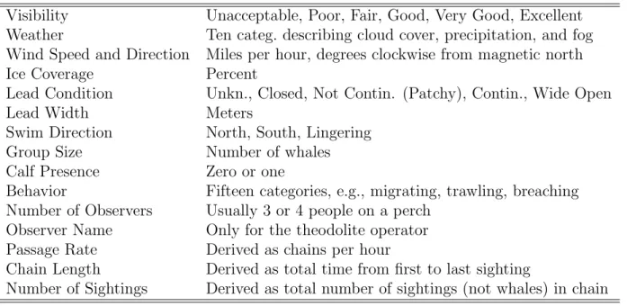
Table 2.2: Main covariates recorded or derived from sightings data in addition to the time, location, and link code.
Visibility Unacceptable, Poor, Fair, Good, Very Good, Excellent Weather Ten categ. describing cloud cover, precipitation, and fog Wind Speed and Direction Miles per hour, degrees clockwise from magnetic north
Ice Coverage Percent
Lead Condition Unkn., Closed, Not Contin. (Patchy), Contin., Wide Open
Lead Width Meters
Swim Direction North, South, Lingering
Group Size Number of whales
Calf Presence Zero or one
Behavior Fifteen categories, e.g., migrating, trawling, breaching Number of Observers Usually 3 or 4 people on a perch
Observer Name Only for the theodolite operator Passage Rate Derived as chains per hour
Chain Length Derived as total time from first to last sighting
Number of Sightings Derived as total number of sightings (not whales) in chain
2.2.4 Data Exclusions
Some data were discarded before estimating detection probabilities: • Closed or indeterminate lead conditions.
• Distances from perch exceeding 4 km, or missing. • Visibility rated as poor or unacceptable.
• Single sightings occurring at times when matching would have been impossible. See Section 2.3.1.
• Unlinked X, R, Y, and Z Duplicates. All of these are re-sightings of previously seen groups or single animals. Therefore, these exclusions do not reduce the number of captures from the perch.
• A handful of sightings where on-perch calculations of distance (using theodolite data and a hand-held calculator) were wildly inconsistent with post-hoc calculations during matching. In half these cases, an obvious single-digit typographical error was corrected; the other cases were discarded.
All results in this paper pertain to the clean dataset. Note that excluding cases while esti-mating detection probabilities does not have any more direct effect on abundance estimation. For the latter task, all the sightings can be used.
2.3 Analytical Methods
2.3.1 Chain Weighting
My analysis weights chains to account for differences in the opportunity to match sightings and the confidence in sightings and matches.
Availability Windows
I begin our discussion of weighting by introducing the concept of IO windows. A period of IO effort usually lasted about 4 hours, although longer and shorter times sometimes occurred. We call these periods ‘IO windows’. For a four hour IO window, we define the first and last hours of the period to be the ‘fringe’. The middle two hours are the window ‘core’. For shorter windows, the core will be smaller or even zero. For longer windows, the core will be greater than two hours but the fringes are always one hour.
Based on average swim rates and the experience of observers and matchers, the opportunity to sight a whale that is matched to another sighting is nearly zero before and after one hour from that sighting. Notwithstanding this, the master matchers examined a much longer time frame (2.5 hours ‘lookback’), yet very few sightings were matched beyond one hour apart.
Note that any unmatched sighting within the IO window core is available for matching dur-ing the entire time when it could potentially be matched. Sightdur-ings in the frdur-inges of the IO window have less opportunity to be matched. A correction should be applied to prevent downward bias in the number of recaptures and corresponding downward bias in estimated detection probabilities.
Call the 2-hour period centered at a sighting (i.e., ±1 hour) the sighting’s ‘availability win-dow’. Then unmatched chains whose availability window is not wholly contained in an IO window might have been matched if IO effort had been expanded. Thus, the evidence such a sighting provides in favor of a non-match is weaker than an unmatched sighting with complete match availability. Weights are assigned to single sightings to reflect this. For a sighting at one perch, define its ‘match availability weight’ to equal the percent of the sighting’s availability window that overlaps with any IO window(s). The simplest example is a case where one perch operates continuously and sights a whale at the exact instant that the other perch ends IO effort. Then this sighting has weight 0.5 because it can be matched backward to the last hour of the IO period but cannot be matched forward to the subsequent hour when the second perch is inoperative. Counterintuitively, a sighting from one perch that occurred outside an IO window may still have some opportunity to be matched: it may be matched to a sighting within an IO window whose boundary is within 1 hour of the outside sighting. Match chains are assigned availability of 1.
Conditional sightings
Another complexity concerns the treatment of chains (including single sightings) involving Conditional sightings. Zeh et al.(1991) and subsequent analyses have treated a Conditional sighting as half a New sighting when estimating detection probabilities and abundance. We too assign a ‘Conditional weight’ of 0.5 to any Conditional single.
Conditional sightings also occur in link chains. For example, consider a sequence of sightings like N1 C1 → X1 where, importantly, the gap indicates that there is no link between the
initial New whale and the subsequent Conditional sighting. The absence of a preceding link is compelled by the definition of the term Conditional, and indeed the earlier New whale is merely implicit in the sense that every Conditional whale has at least one New or Duplicate whale before it. Assigning equal odds for a Conditional being New or Duplicate, the above sequence of sightings can be interpreted in two ways. With probability 0.5 the Conditional has not been previously seen so the sequence is equivalent to N1 N1 → X1. On the other
hand, with probability 0.5 the Conditional is actually a re-sighting of some previous whale, in which case the sequence is equivalent to N1 → X1 → X1 for some preceding N1. Thus a
Conditional link chain is also half a sighting.
Treating match chains with leading Conditional sightings at one or both perches is more complex–particularly because the chain must be weighted as a single unit rather than weight-ing the sightweight-ings from each perch separately. Nevertheless, we can apply analogous reasonweight-ing to show that we should use Conditional weights of 0.75 if one of the matched sightings is Conditional and 0.5 if both are.
Match uncertainty
Section 2.2.2 explained the Excellent, Good, and Average ratings the master matchers used to rate their confidence in each match. I will associate probabilities pE, pG, and pA to the
three types of matches to indicate the probability that the declared match is correct. In our baseline analysis, we will let pE = 1, pG = 0.78, and pA = 0.58, with the latter two
values chosen to be the midpoints of the respective confidence ranges used by the matchers. Sensitivity to these choices is explored in Section 2.4.2.
These match confidence probabilities pertain to matched sightings, not complete match chains. When one considers that each match connection in a match chain may or may not be correct, it is clear that any observed match chain could be a flawed observation of an underlying truth. Many possible changes to the match calls, in isolation or combination, create alternative configurations of the relevant sighting data, and each configuration can be associated with a corresponding probability weight. Specifically, the other configurations can be enumerated by considering all possible combinations of ‘retaining’ and ‘breaking’ declared
matches, and the probability of each resulting configuration can be derived using pE, pG,
and pA.
Consider the match chain N1 A
⇔ N2 G
⇔ C1 where the letters above the match arrows indicate
match quality ratings. Table 2.3 lists the possible alternative configurations for this match chain, and the corresponding probabilities. Note that when pE = 1, as for our recommended
analysis, Excellent matches are never broken.
For any chain or alternative configuration, define its ‘match confidence weight’ to be the probability of that configuration using the probabilities discussed here, such as the example in Table 2.3. For statistical modeling and analysis, each match chain is replaced by the set of possible configurations, each assigned its corresponding match confidence weight. Finally, I note that the original chain always receives the highest probability since all the match confidence probabilities exceed 0.5.
Replacing match chains with sets of chain configurations weighted by their probabilities may seem to be a bold departure from the raw data until one can witness the actual matching process. To a master matcher, such an approach seems not only sensible but essential. The
Table 2.3: Possible alternative configurations and probabilities for the match chain N1 A
⇔ N2
G
⇔ C1 where the letters above the match arrows indicate match quality ratings. The
original chain is most likely and is listed first.
N1 ⇔ N2 ⇔ C1 pApG
N1 N2 ⇔ C1 (1 − pA)pG
N1 ⇔ N2 C1 pA(1 − pG)
N1 N2 C1 pApG
master matchers can spend up to 1 hour agonizing over just one potential match decision and debating match confidence ratings as they pore over the data. When they decide to declare a match and rate it as Good, they are relying on that confidence rating and its quantitative de-scription (e.g., ‘at least 66% confidence’) to express their very real uncertainty about the call.
Summary of weighting
In summary, there are three factors that can affect how a chain is weighted. First, the concept of availability is used to adjust sightings made when there was a reduced recapture opportunity due to the timing of IO and single perch effort. This must increase detection probability estimates. Second, the traditional half-weighting of Conditional sightings is applied to single and link chains, with analogous extensions to match chains involving one or more Conditional sightings in a match. This weighting should be roughly neutral with respect to detection probabilities. Third, match chains are weighted by their match confidence. This has a negative effect on detection probabilities. The overall weight for a chain is defined to be the product of these three weights, with the match confidence weighting implemented using the alternative configuration method in Section 2.3.1.
2.3.2 Group Size Consistency
Each recorded sighting may be of a single animal or a group. These groups are not whale pods in the conventional sense. Except for cow-calf pairs, migrating bowheads appear to
have only weak and probably brief allegiance to any aggregation but their associations are not purely random (Zeh et al., 1993). When the number of whales in a sighted group (‘group size’) is seen to vary along a chain, this may be attributable to whales joining or leaving a chain, and/or to variation in detection. A poll of observer opinions after the survey finds divided views, with some observers tending to attribute group size inconsistencies to a fail-ure to detect group members, and others tending to attribute it to whales (‘transients’) joining or leaving groups. Group size inconsistencies are relatively common among match chains. Indeed, 574, 109, 16 and 5 match chains had (maximal) group size inconsistencies of 0, 1, 2, and 3 whales, respectively. This corresponds to an inconsistency rate of 18.5% for match chains. The most common inconsistency is a group size 1 matched to a group size 2.
Along with distance, group size is a dominant factor influencing detection probabilities. The fact that animals may join or leave a chain during the period that the chain is (repeatedly) sighted is of paramount importance because estimation of detection probabilities fundamen-tally relies on counts of captures and recaptures. When group sizes in a chain vary, these counts are uncertain. Thus, resolving group size inconsistency is a major dilemma that must be addressed in the analysis. It is clear that analysis methods that recognize these potential fleeting group allegiances better reflect the behavioral processes that generate the observed data.
We must also recognize that whales are not individually sighted. For the bowhead survey, capture and recapture events pertain to groups, not individuals. Groups are sighted and recorded on the perches, and groups are plotted and matched during the post-hoc matching phase. All the approaches I will describe below embrace this fact: I will estimate detection probabilities of groups. However, this does not require me to ignore group size inconsistency, nor should I. Nevertheless, the first approach I apply for dealing with group size inconsis-tency is to ignore it. I label this method ‘Inconsistent’. This approach amounts to assuming
that there are never transient departures or joinings to a group. Next, I introduce another strategy I call ‘deconstruction’ to model the possibility of transient group affiliation. With this approach, I may isolate certain possible transients, thereby decomposing a match chain into several parts.
To explain deconstruction, I first define a sub-chain of an original chain to be any chain of connected sightings (links and/or matches) from the original chain with consistent group size that can be obtained by reducing the group sizes at any chosen sightings in the original chain. A chain can be decomposed into a unique set of group size consistent sub-chains by sequentially removing the longest chains of each possible group size, starting with the largest group size and working downward. For example, the sub-chains of a chain having group sizes (2,1,1,2,2) in that order are the chains (1,1,1,1,1), (1,0,0,0,0), and (0,0,0,1,1) where ‘0’ indicates absence of chain membership.
Deconstruction identifies sub-chains of link and match chains that can be reasonably at-tributed to transients. The following is a deconstruction method based on mode chain group size.
1. Calculate the mode m of group sizes for sightings comprising the chain. (Suppose here that we are beginning with a match chain.) The mode is chosen to be a reasonable estimate of the true group size.
2. Replace all group sizes less than m in the chain with m. 3. Set aside the sub-chain having consistent group size m.
4. Subtract m from the group size of each sighting in the original chain. Remove from the chain any sightings with group size 0.
5. Break all remaining matches in the original chain, if any. Although we break these matches, the remnant group sizes are unchanged.
6. What remains, if anything, will be a collection of isolated (i.e., unlinked) groups and link chains with sightings, possibly with inconsistent sizes.
7. Repeat the above steps separately for each link chain. No repetition is needed for any single group because it already has consistent group size. Continue iterating this process within each sub-chain, and for every sub-chain, until what remains is a set of chains all having internally consistent group sizes, including the original chain with the mode group size.
An elaborate example of deconstruction is presented by the chain having the sequence of group sizes (2,3,1,1,1,3,3,4,4). The longest sub-chain we can extract with consistent group size is (1,1,1,1,1,1,1,1,1), assuming we define the mode to be 1. Subtracting these whales leaves (1,2,0,0,0,2,2,3,3), which must be further deconstructed. The next sub-chain is (0,0,0,0,0,2,2,2,2) since we attack the right hand remnant first. Continuing in this fashion yields the remaining components: (1,1,0,0,0,0,0,0,0), (0,1,0,0,0,0,0,0,0), and (0,0,0,0,0,0,0,1,1). This example is for illustration; most real chains are far simpler.
It is possible that the subtraction step #4 may leave match connections between sightings of non-zero group sizes. The reason that these matches are broken in step #5 is because the original chain represents one recapture event. Failing to break remnant match sub-chains would count the match event more than once.
The mode group size may be a tie between two values. Accordingly, I define two alternative methods: ‘Decon↓’ rounds modes downward, and ‘Decon↑’ rounds upward.
Deconstruction both subsumes and creates transients. In step #2, whales are added to match chains to represent true group members that were undetected. In steps #4-6, the ex-tra chains (if any) produced represent whales having ex-transient memberships to the true group recaptured. This approach is a compromise between assuming that every chain represents
the largest possible group with no transients and assuming that every chain corresponds to the smallest group size seen with all remaining whales being transients. Finally, recall that group size is a direct observation, not a derived variable. The observers are making an explicit statement about what they see. An appealing aspect of deconstruction is that field observations are taken at face value rather than second-guessing the trained observers after the fact.
The choice between the three methods (Decon↑, Decon↓, and Inconsistent) is a choice about how to count captures and recaptures. Each of the three methods makes a different as-sumption about transients–from none to many–and each of these asas-sumptions leads to the addition of some number of single chains (or none) to represent transient whales. This is unrelated to how whales are counted for the purpose of making an abundance estimate. It is also unrelated to how group size is assigned to a chain as its covariate value for estimation of detection probabilities. As described in Section 2.2.3, the group size covariate value is defined to be the size observed at the first recapture event. The same group size covariate value is assigned to any sub-chains of the original chain. This is the most appropriate choice because detection probabilities relate to detection of groups.
2.3.3 Detection Probability Estimation
I adopt the model of Huggins (1989) for capture-recapture estimation for closed populations. This model assumes that captures at each perch are independent and that the catch history is therefore multinomial for each individual. To form the likelihood, the model conditions on the total number of groups detected. We constrain our analysis to assume that probabilities are equal among the perches. The detection probability for a group is allowed to depend on covariate observations for that group. The effect of covariates is the primary focus of our analysis.
Models are fit using the MARK software (White and Burnham, 1999), using the RMark interface (Laake, 2011). However, all of the analyses described here include considera-tion of weighted observaconsidera-tions. A method for weighted fitting of the Huggins model using MARK/RMark is given next.
Fitting weighted capture - recapture models with MARK
Models are fit using the MARK software (White and Burnham, 1999), using the RMark interface (Laake, 2011). However, all of the analyses described here (except G0) include
consideration of fractional whales, which is equivalent to weighted observations. This sec-tion provides more details and describes a method for obtaining the results of the weighted analysis using the MARK program, thereby circumventing the need to develop a customized estimation procedure. The key results are given in equations (1), (2), and (3). Although I refer to MARK results below, it is easiest to implement these ideas using RMark, from which the necessary quantities can easily be extracted and manipulated.
Weighted observations
Suppose we wish to assign the ith outcome (i.e., the catch history for a single, link, or match chain) a weight wi for i = 1, · · · , n where n is the sample size and, without loss of generality,
0 < wi ≤ 1. Our method temporarily replaces the original, unweighted dataset with a larger
dataset that replicates the ith observation ri times, where ri = Rwiand R is chosen to be the
smallest integer such that riis an integer for all i . Thus the total sample size in the expanded
dataset is nR= n P i=1 ri = R n P i=1
wi. If the desired weights are rounded to the first decimal place,
then R ≤ 10. In an analysis where the presence of conditional whales requires wi = 1, 0.5, 0.75
There are several instances where weighting may be used. Consider Conditional sightings, i.e., sightings where the observer cannot determine whether the whale is New or a Duplicate. Zeh et al. (1991) and subsequent analyses have treated a single Conditional whale as half a New whale when estimating detection probabilities and abundance. Thus we assign weights of 0.5 to conditional sightings here.
Conditional whales in link and match chains must also be addressed. For example, consider a sequence of sightings like N11 C11 → X1
1 where, importantly, there is no link between the
initial New whale and the subsequent Conditional sighting. The absence of a preceding link is compelled by the definition of the term Conditional, and indeed the earlier New whale is merely implicit in the sense that every Conditional whale has at least one New whale at some earlier time. Assigning equal odds for a Conditional being new or duplicate, the above sequence of sightings can be interpreted in two ways. With probability 0.5 the Conditional has not been previously seen so the sequence is equivalent to N11 N11 → X1
1. On the other
hand, with probability 0.5 the Conditional is actually a resighting of some previous whale, in which case the sequence is equivalent to N1
1 → N11 → X11 for some preceding N11.
Assume the simplest possible capture-recapture model with the probability of capture at each perch and the probability of recapture all equal to p. Then the first possibility represents two whales, thereby contributing p2 to the likelihood. The second possibility represents a single whale contributing p to the likelihood. In the next section we develop a method allowing one to assign a weight of 0.5 to a Conditional whale by letting it contribute p × p12 = p
3 2 to
the likelihood. This approach is also consistent with the standard principle of weighting ob-servations in statistical models: that a random variable having half the weight is equivalent to having twice the variance.
The weight of 0.5 is used for Conditional sightings that are unconnected or which lead a link chain. Treating match chains with leading Conditional sightings at one or both perches is more complex - particularly because the chain must be weighted as a single unit rather than weighting the sightings from each perch separately. Nevertheless, we can apply analogous reasoning to show that we should assign such chains a weight of 0.75 if one perch reported Conditional and 0.5 if both perches reported Conditional.
Weighting and MLEs for exponential families
I now discuss my weighting approach in the context of exponential families. For exponential family distributions with weighted observations, there is a useful relationship between certain likelihoods. In the simplest and most generic case, a density in the exponential family can be written as
f (xi|θ) = exp{
xiθ − b(θ)
φ/wi
+ c(xi, φ/wi)}
where φ is a fixed dispersion parameter and wi is a known weight. The exponential family
includes many familiar distributions including the Gaussian, binomial, and multinomial dis-tributions; the latter two are directly relevant for capture-recapture models.
Consider the simplest (i.e., null) Huggins Huggins (1989) model with one recapture oppor-tunity. Each weighted observation in the dataset (e.g., each catch history) contributes a term to the likelihood function used to estimate the model. Denote the corresponding log likelihood contribution as
li(θ|xi) = wiAi+ c(xi, φ/wi)
Ai = (xiθ − b(θ))/φ, θ = log(p/(1 − p)), b(θ) = − log(2 + exp{θ}), φ = 1 and xi equals 1
if the catch history does not include a recapture and 0 otherwise. For an i.i.d. sample, the overall log likelihood is the sum of such contributions, namely
l(θ|X) = n X i=1 li(θ|xi) = n X i=1 wiAi+ q
where X = xi, · · · , xn represents the entire dataset and q is a constant that does not depend
on θ.
Let XR represent the dataset where each xi is replicated ri times and there is no weighting
of the observations within XR. Let xi,ji for ji = 1, · · · , ri denote these replicates of the ith
case in X. Then the contribution to the overall unweighted log likelihood lR(θ|XR) for xi,ji
is
lR,i,ji(θ|xi,ji) = Ai+ c(xi,ji, φ)
and the total contribution associated with the ith catch history is
ri
X
ji=1
(Ai+ c(xi,ji, φ)) = riAi+ qR,i
where qR,i is a constant that doesn’t depend on θ. It follows that the overall log likelihood
given by the unweighted, replicated dataset is
lR(θ|XR) = R n
X
i=1
where q∗R doesnt depend on θ.
Our key results follows from the fact that terms not involving θ are irrelevant when computing the score functions from l(θ|X) and lR(θ|XR). Specifically,
dl(θ|X)
dθ =
dlR(θ|XR)/R
dθ
Thus the MLE for the weighted likelihood equals the maximizer of the replicated likelihood, i.e.,
ˆ
θM LE = ˆθR (2.1)
Although this discussion is presented for unidimensional θ, the analogous results for vector parameters are obvious. Because it is based on the multinomial distribution, the results above pertain to the general Huggins (1989) model, including the case when detection prob-abilities are modelled to depend on a collection of covariates. The covariates inherent in the model lead one to express the parameter vector in the conditional likelihood as a function of the coefficients in the linear predictor portion of the model. The standard maximum likelihood assumptions are also implicit above and in what follows.
Computing AICc differences
Consider the comparison of two fitted models, which we will represent as ˆθ1 and ˆθ2,
recog-nizing that the two models may have different parameter sets. Define