THESIS
A GPU ACCELERATED RNA-RNA INTERACTION PROGRAM
Submitted by Brandon Gildemaster Department of Computer Science
In partial fulfillment of the requirements For the Degree of Master of Science
Colorado State University Fort Collins, Colorado
Spring 2021
Master’s Committee:
Advisor: Sanjay Rajopadhye Hamidreza Chitsaz
Copyright by Brandon Gildemaster 2021 All Rights Reserved
ABSTRACT
A GPU ACCELERATED RNA-RNA INTERACTION PROGRAM
RNA-RNA interaction (RRI) is important in processes like gene regulation, and is known to play roles in diseases including cancer and Alzheimer’s. Large RRI computations run for days, weeks or even months, because the algorithms have time and space complexity of, respectively, O(N3M3) and O(N2M2), for sequences length N and M , and there is a need for high-throughput RRI tools. GPU parallelization of such algorithms is a challenge.
We first show that the most computationally expensive part of base pair maximization (BPM) algorithms comprises O(N3) instances of upper banded tropical matrix products. We develop the first GPU library for this attaining close to theoretical machine peak (TMP). We next optimize other (fifth degree polynomial) terms in the computation and develop the first GPU implementation of the complete BPMax algorithm. We attain 12% of GPU TMP, a significant speedup over the original parallel CPU implementation, which attains less than 1% of CPU TMP. We also perform a large scale study of three small viral RNAs, hypothesized to be relevant to COVID-19.
TABLE OF CONTENTS
ABSTRACT . . . ii
LIST OF TABLES . . . v
LIST OF FIGURES . . . vi
Chapter 1 Introduction . . . 1
Chapter 2 Related Work . . . 4
Chapter 3 BPMax . . . 5
Chapter 4 Background . . . 9
4.1 Parallelization of an RRI surrogate . . . 9
4.2 A Tropical Multi-MatMult Library . . . 10
4.3 GPUs and Thread Divergence . . . 11
Chapter 5 Banded Tropical Matrix Multiplication . . . 15
5.1 Padding . . . 15
5.2 First Approach . . . 17
5.3 Improved Banded Library . . . 18
5.3.1 Banded Matrix Memory Layout . . . 19
5.4 Library Modifications . . . 19
5.5 Mapping Linear Addresses . . . 21
5.6 Correctness considerations . . . 23
Chapter 6 BPMax: The Remaining Terms . . . 24
6.1 Optimizations . . . 24
6.2 H1 and H2 . . . 26
6.3 H3 and H4 . . . 26
Chapter 7 Experimental Results . . . 28
7.1 Performance Benchmark Considerations . . . 28
7.2 Triangular Matrix Performance . . . 29
7.3 Varying the Matrix Size and GPU Parameters . . . 30
7.4 Banded Matrix Performance . . . 33
7.5 Varying the Window Size . . . 33
7.6 Performance ofH1throughH4 . . . 35
Chapter 8 SARS-CoV Data Set . . . 37
Chapter 9 Full BPMax Performance . . . 38
Chapter 10 Conclusion and future work . . . 41 Bibliography . . . 43
LIST OF TABLES
LIST OF FIGURES
3.1 Eddy-Rivas diagram. . . 6
3.2 4D dynamic programming table depiction and double reduction computation pattern . 8 4.1 Illustration of a grid of CUDA thread blocks. . . 14
5.1 Padding visualization . . . 16
5.2 Double reduction library call and computation structure . . . 17
5.3 Thread block data layout scheme and logical thread block mapping. . . 20
5.4 Mapping 1D addresses to 2D addresses. . . 22
6.1 Single strand folding methods. . . 25
7.1 Banded matrix multiplication library performance for triangular matrices . . . 30
7.2 Performance across three GPU architectures . . . 31
7.3 Banded matrix multiplication speedup vs. square library . . . 31
7.4 Banded matrix library effective performance varying matrix sizes and number of threads 32 7.5 Banded matrix multiplication library performance restricted window size . . . 34
7.6 Banded library performance for varying window size . . . 34
7.7 H1, H2 Performance . . . 35
9.1 Performance of full BPMax . . . 39
9.2 BPMax GPU run time . . . 39
Chapter 1
Introduction
RNA molecules comprise a sequence of four different nucleotides: adenine, uracil, guanine and cytosine (A, U, G, C). An RNA molecule can form intra-molecular bonds (base pairs) between its nucleotides, or form inter-molecular bonds with other RNA molecules. The result of such interac-tion is called the secondary structure. Knowledge of this structure can provide useful informainterac-tion about biological function, and may be used in experiments [1, 2].
RNA-RNA Interaction (RRI) algorithms like piRNA [3], IRIS [4], RIP [5] and the recent BP-Max and BPPart [6] follow recurrences similar to those of single strand RNA folding [7, 8], but are computationally more expensive: the time and space complexities, for sequences lengthN and M , are O(N3M3) and O(N2M2), respectively. Moreover, the constant factors may vary by two orders of magnitude, and the largest sequences that can currently be handled by piRNA are only a few hundred nucleotides (nt) long, and this is more due to memory constraints than computational resources.
To the best of our knowledge, there is no work on parallelizing any of the RRI algorithms except for a naive OpenMP parallelization of the original piRNA and RIP, whose limitations we discuss later. They both incorporate thermodynamic information, and use 96 different dynamic programming tables. This large memory requirement makes them even more challenging than single strand folding, especially on accelerator platforms like GPUs. Indeed, implementing piRNA on a GPU is out of reach of current GPU hardware. BPMax [6] is an RRI algorithm based on a weighted base pair counting model, and it only requires a single dynamic programming table, and thus far less memory, albeit by a constant factor. This makes GPUs much more feasible targets for BPMax, compared to the more complex counterparts.
In this paper, we develop efficient GPU parallelization of BPMax. The strategy is very different from the standard, “diagonal-by-diagonal” one used for such algorithms, be they for single RNA or for RRI. We first describe how a somewhat non-standard view of the recurrences allows us to
describe the dominantO(N M )3 core of the algorithm asO(N )3 instances of the product of two M × M matrices in the max-plus semiring (also called the tropical semiring). Amongst these multiple instances, there is a parallel structure similar to that in the single-stand algorithms and in particular, the computation proceeds in a quadratic sequential loop, by simultaneously invoking O(N ) independent instances of the max-plus semiring matrix product. We therefore first developed a library to perform multiple independent tropical semiring matrix products, specialized for upper banded matrices.
The next most computationally expensive portion of BPMax, an O(N2M3) computation, is almost identical to O(N )2 instances of the more simple single strand folding algorithm. Rizk et al. [9] designed an optimized GPU program for single strand RNA folding which was further refined by Li et al. [10]. We developed a library similar to these techniques, but which executes
multiple instances, and integrated it with BPMax.
The run time for input RNA sequences typical of a SARS COVID-19 data set of recent im-portance (see Chapter 8) was 3056 seconds on a high end modern CPU for the original BPMax implementation, and our optimized GPU algorithm processes this problem in just 4.79 seconds. For that data set the original implementation attains less than 1% of theoretical machine peak op-erations per second on all problem instances, while our GPU algorithm reaches around 12% of machine peak for the relevant data set. Our GPU algorithm attains 50% of machine peak on other input sizes. Our specific contributions are as follows
• We show how the most computationally expensive part of RNA-RNA interaction base pair maximization algorithms can be expressed as a collection of tropical semiring matrix mul-tiplications on upper banded matrices by applying memory transformations to the dynamic programming table.
• No existing GPU library performs the multiplication of two upper banded matrices, therefore we developed the first such optimized library and show it attains 6x speedup over a library optimized for square matrices.
• We create the first GPU implementation of an RNA-RNA interaction algorithm.
• Our GPU program attains significant speedup over the original CPU implementation, which enables us to perform a large scale study of three CoV-SARS-2 svRNA sequences.
The rest of this thesis is organized as follows: chapter 2 describes related work and provides context for where our contributions fit into the existing literature. Chapter 3 explains the recur-rence equations involved in BPMax and the strategy we use to compute the most significant term. Chapter 4 recalls previous work on parallelizing a program with the same dependence patterns all dynamic programming RRI algorithms follow, and describes special considerations for a GPU parallelization. Additionally, this chapter describes the first step towards our goal, the develop-ment of a tropical matrix multiplication library operating on square matrices, and chapter 5 then describes the modifications done to make the library optimized for triangular and upper banded matrices. Chapter 6 explains the rest of the GPU implementation of BPMax, and in chapter 7, we benchmark performance for each GPU library call individually, and report end-to-end perfor-mance of the entire integrated application. In chapter 8 we present the data set used for end-to-end performance evaluation, showing real value in a practical use case, and report performance for the dataset in Chapter 9. Chapter 10 gives conclusions and future work for BPMax and other RNA-RNA interaction programs.
Chapter 2
Related Work
Nussinov introduced a dynamic programming algorithm in 1978 which predicts the secondary structure of a single RNA molecule [7]. The Nussinov algorithm computes the most probable structure as the one that maximizes the number (or more precisely, the weighted sum) of base-pairs that form a chemical bond. It hasO(N3) time and O(N2) space complexity. Further work by Zuker and Stiegler [8] incorporated a thermodynamic energy model which produces more accurate results with a constant factor extra work. Most algorithms use the metrics introduced in these papers, either base-pair maximization (BPM) or free energy minimization (FEM) and much work has been done optimizing and parallelizing variations of these algorithms for CPU platforms [11, 12], and Rizk et al. [9] present a GPU implementation of Zuker’s algorithm, and Chang et al. [13] include a BPM version of the algorithm. Other work by Li et al. includes both CPU and GPU parallelizations of BPM [10].
Chapter 3
BPMax
A large body of past work casts a family of similar dynamic programming problems as semiring matrix multiplication. Maleki et al. propose a parallelization strategy for dynamic programming problems such as Viterbi, Needleman-Wunsch, Smith-Waterman, and Longest Common Subse-quence [14] that involves expressing most of the computation as such matrix multiplications, fol-lowed by a fix-up phase. The all-pairs shortest-paths problem has a similar structure, and optimal versions of this algorithm on a GPU utilize max-plus matrix multiplication [15]. Matrix multiplica-tion strategies have been applied to single strand RNA folding as well. Valiant showed context-free grammar recognition is equivalent to Boolean matrix multiplication [16], and further work pro-vides a link between RNA folding and context-free grammars [17, 18]. Zakov et al., then applied Valiant’s approach for parsing a context-free grammar to RNA folding, reducing the asymptotic run time for the algorithm to sub-cubic matrix multiplication [19]. All of these algorithms work on a 2D dynamic programming table. We build on this past work, and extend the matrix multiplication formulation to the 4D dynamic programming table used in RRI.
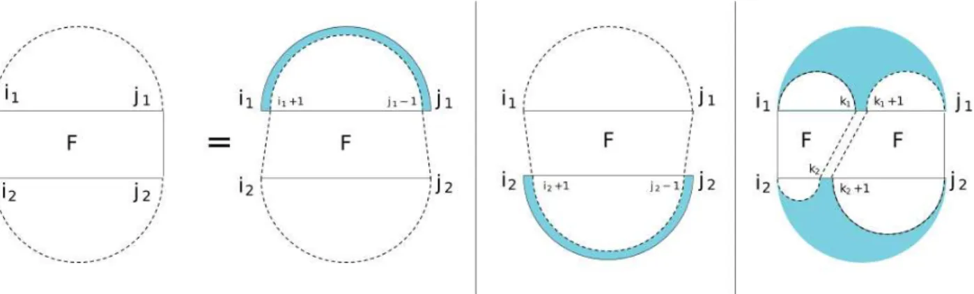
BPMax, BPPart and piRNA/RIP [5, 6] are all very similar dynamic programming algorithms for RRI, with the same asymptotic complexity, albeit with significantly different constant factors. BPMax is the simplest, and performs weighted base pair maximization, similar to Nussinov’s algorithm for single strand folding [7]. It produces a four dimensional table, F , which gives an interaction score of the input RNA molecules. A higher score implies a more stable molecule, and the table can also be backtracked to recover structural information. BPMax considers both inter-molecular and intra-molecular base pairings, and does not allow pseudo-knots or crossings. Figure 3.1 depicts, using the Rivas-Eddy diagrams [20] common in the bioinformatics community, the three main cases for computing a value in theF table (the diagram is to be seen as the rules of a context free grammar.
Equation 3.1 gives the full recurrence equation for BPMax. It specifies the elements of a 4-D table, viewed as an upper triangular array, each of whose elements is itself a triangular array. S(1) andS(2)are tables for each strand, whose value athi, ji gives the maximum weighted sum of base pair scores on all possible foldings of the single sequence, using the classic Nussinov algorithm. The boxed term in the recurrence is the dominant term, takingO(N3M3) time.
Figure 3.1: The four cases defining table F.
Fi1,j1,i2,j2 = iscore(i1, i2) i1 = j1 and i2 = j2 max j1−1 max k1=i1 j2−1 max k2=i2 (Fi1,k1,i2,k2 + Fk1+1,j1,k2+1,j2) , j2−1 max k2=i2 (Fi1,j1,i2,k2 + S (2) k2+1,j2), j2 max k2=i2 (Fi1,j1,k2+1,j2 + S (2) i2,k2), j1 max k1=i1 (Fk1+1,j1,i2,j2 + S (1) i1,k1) j1 max k1=i1 (Fi1,k1,i2,j2 + S (1) k1+1,j1) Fi+1,j−1,i2,j2 + score(i1, j1), Fi1,j1,i2+1,j2−1+ score(i2, j2) otherwise (3.1)
In the rest of this paper, the boxed term is called the double reduction. Similarly,H1, H2, H3, andH4, successively, refer to the terms below the boxed term, each of which is a single reduction. Note that the asymptotic complexity of these terms is a 5-th degree polynomial, eitherO(N2M3) orO(N3M2). The remaining three terms are simple constant time look-ups using the score and iscore functions.
For many practical inputs, the memory footprint for sequences of even a few hundred nt is prohibitive, so the authors proposed a windowed version of the algorithm which limits intra-RNA interactions to only be allowed if the indices are within a predetermined window (usually specified as a fraction α1 of the sequence length). The windowed version leads to a trapezoidal array of trapezoids, or equivalently upper banded matrices. In this version the computational complexity is reduced by a factor of 2α32, and the memory footprint by a factor of α42 over those of the triangular version. Such windowing arguably reduces the accuracy of the prediction, but is widely accepted in the community. Indeed, Fallmann et al. [21] claim that for intra-RNA interactions, locally stable structures are typically formed rather than structures folded globally, and Lange et al. [22] even observe this empirically for a class of RNA. The windowed version of BPMax does just this, while allowing and arbitrary distance for inter-RNA interactions.
There is a very simple direct parallelization of the RRI algorithms. Just like in a single RNA secondary structure, corresponding to a “diagonal-by-diagonal” evaluation within each triangle, and the triangles themselves evaluated in a “diagonal-by-diagonal” order, and this was imple-mented by the authors of piRNA and RIP. However, this parallelization strategy (only) seeks max-imum parallelism, and has very poor locality at all levels of the memory hierarchy of modern processors, and also does not exploit their high degree of fine grain, vector processing capabilities. Indeed, when the memory footprint exceed the DRAM capacity, and uses virtual memory, the disk thrashing caused by these programs render the machine completely unresponsive and requires a manual reboot by system administrators.
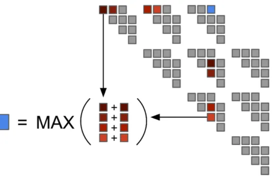
The 4-D dynamic programming table is shown in Figure 3.2. The outer dimensions,i1 andj1, define a trapezoidal grid of trapezoidal (i.e., upper banded) matrices and the inner two dimensions,
i2 and j2, are points within the matrices. The size of the trapezoidal grid isN × N and the size of a matrix in the grid isM × M for sequences length N and M . For each memory location in the table, each term in the recurrence equation is evaluated.
The double reduction term contributing to the blue cell is the dot product, using max plus operations, of the row of red colored cells (of different shades) to the left of the blue cell and the column of red cells below it.
Chapter 4
Background
We now recall previous work on parallelizing a program withO(N3M3) complexity that is a surrogate for the dependence patterns in all RRI algorithms and also describe some special con-cerns with GPU parallelization.
4.1
Parallelization of an RRI surrogate
Varadarajan [23] investigated the parallelization of piRNA, and as a first step, defined a sim-plified surrogate miniapp called (OSP)2 that had the dependence patterns similar to piRNA. It updates a triangular collection of triangular arrays of double precision floating point numbers, using the following specification,
T [i1, j1, i2, j2] = k1=j1−1,k2=j2−1 X k1=i1,k2=i2 mT [i1, k1, i2, k2] ∗ T [k1+ 1, j2, k2+ 1, j2] (4.1)
This equation is very similar to the double reduction in BPMax, except that it manipulates dou-ble precision floating point numbers, approximation linear algebra computations in the real field, whereas the BPMax equation performs the corresponding operations on integers in the max-plus (tropical) semi-ring. Varadarajan observed that the state of the art polyhedral compiler Pluto [24] was unable to exploit locality, giving no improvement over the baseline. She then applied semi-automatic transformations using the AlphaZ system for polyhedral program optimization, devel-oped at CSU [25]. She showed that a carefully chosen set of loop permutations was able to obtain a very impressive speedup of more than100× over the baseline. She was also able to show through a roofline analysis [26] that the performance attained the theoretical limit of the bandwidth of the L1-cache. The main reasons for the impressive performance gains were exploiting locality, and
both coarse grain (across multiple cores) and fine grain (vector) parallelism. As we will see later, this naturally lead towards the view the computation as collections of matrix products.
4.2
A Tropical Multi-MatMult Library
When the set of transformations that gave good performance on Varadarajan’s(OSP)2miniapp were analyzed, the common features in all of them were that (i) the innermost loop was vectoriz-able, and had good locality, and (ii) the outer three loops were some permutation of thei1, j1 and k1 indices. Thus, the innermost three loops were efficiently computing
k2=j2−1 X k2=i2
T [i1, k1, i2, k2] ∗ T [k1+ 1, j2, k2+ 1, j2]
Observe that ifi1,j1,k1are fixed, this is very similar to matrix product. In fact, it is the product of thehi1, k1i-th submatrix of T with its hk1 + 1, j1i-th submatrix. Vardarajan found that in the outer three loops iterating over complete triangles, if thek1 loop is moved out to the middle and kept sequential, the outermost (sequential loop) is made to iterate diagonal by diagonal, and the innermost (j1) loop made parallel, for every diagonal a set of multiple independent matrix products is performed. This is the key idea of our parallelization strategy.
Using this insight for BPMax, Ghalsasi developed a highly optimized library for multiple instances of matrix products in the tropical semiring [27]. Ghalsasi first wrote a set of micro-benchmarks to determine the attainable peak performance of the max-plus operation on GPUs, and used that to develop a tropical matrix multiplication library for square matrices.
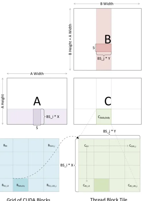
To give a high level overview of Ghalsasi’s matrix multiplication algorithm, figure 4.1 illus-trates the grid of thread blocks, how the thread blocks are mapped to the matrix, as well as the matrix multiplication algorithm. Matrices A, B and C are allocated in global memory on the GPU, then a two dimensional grid of thread blocks is launched for the library call. Each thread block is responsible for computing a patch of the C matrix. To compute the patch of C, the threads in a thread block cooperatively load a patch of A and a patch of B into shared memory. After this step, each thread is responsible for computing partial answers for an area of the patch of C from
the values loaded into shared memory. The main outer loop loads a patch of A and patch of B into shared memory, synchronizes the threads, then computes partial answers for the patch of C that particular thread block is responsible for. The next iteration loads the next patch of A and B and multiplies them until full answers are computed for the patch of C.
To support multiplying multiple parallel instances of matrices, a three dimensional grid of thread blocks is launched rather than a two dimensional grid. The size of the third dimension of blocks is equal to the number of matrices in each column, so the first block in the third dimension multiplies the first matrices in each column as described above and so on. As we report later, this library attain near-peak performance on modern family of GPUs, but cannot be directly used for BPMax.
The library handles only full (square) matrices, and the iteration space of square matrix mul-tiplication is a cube dimensions N3. On the other hand, the iteration space of triangular matrix multiplication is a half pyramid of only one-sixth the volume, and so the library would perform a lot of redundant computation. Even more unnecessary work is done for banded matrices as the window size is reduced.
4.3
GPUs and Thread Divergence
GPU threads have a very different architectural implementation than CPU threads. On a GPU, threads are grouped into units of 32 by the hardware, called a warp, and there is one single program counter for the entire warp. The program counter loads an instruction, and all threads in the warp then execute that instruction. In a for loop when all threads do not need to execute a particular loop iteration, a masking procedure is run to determine which threads should be active for that iteration, and threads that should not execute the instruction are essentially turned off. Warps are further grouped into a coarse grain parallel abstraction called a thread block. A thread block can contain up to 1024 threads in recent GPU architectures, and therefore can comprise up to 32 warps. At run time, a 1D, 2D or 3D grid of thread blocks may be launched with a GPU call, the dimensions of which are controlled by the programmer. For matrix multiplication, typically a 2D grid of thread
blocks is launched, the dimensions of which would correspond to the dimensions of the matrix. A 1024× 1024 matrix can be logically broken up into tiles of size 64 × 64 for example, so a grid of 16 × 16 thread blocks would be launched, each block responsible for computing a 64 × 64 patch of the matrix. All warps within a thread block are ultimately scheduled to run on a streaming multiprocessor (SM) by the run time environment, and an SM may have multiple active warps. The main point of having multiple active warps per SM is to hide instruction latency. If threads in one warp request values from global memory, threads in another warp may run on the SM while the data is fetched. However, having too many active warps on an SM may degrade performance, as each SM has a limited number of resources like registers and shared memory space. After a GPU library is written, the performance can vary greatly by tweaking parameters such as the number of threads per thread block, how many elements each thread should compute in the matrix, the amount of shared memory allocated to each thread block and so on. The search space for parameters that will give optimal performance for a given problem instance is very large, and ways to deal with selecting parameters that will perform well across many problem instances is an interesting topic in its own. We discuss how we select these parameters in chapter 7.
Bialas and Strzelecki [28] benchmark the cost of thread divergence and show the overhead for the masking procedure is significant. Implementing an algorithm where each thread computes a cell in the table from Figure 3.2 and does the exact number of operations required by the equation would incur much overhead, because the masking procedure would run for each iteration of the innermost loop. Threads do not simply sit idle after they have completed their loop iterations, the threads are active until the thread with the most work to do in the warp is completed, and furthermore having threads sit idle introduces overhead which makes the entire warp run longer. If the programmer can have each thread execute the number of loop iterations equal to the thread that has the most work to do in the warp, without affecting the result of the computation in the process, the warp will complete faster than if threads sit idle after they are done.
For BPMax, the amount of work done by the double reduction is different for different cells in the table. Computing the answer for the blue cell in Figure 3.2 requires four max-plus operations
while computing the answer for the cell directly below the blue one would require two max-plus operations. This means threads from the same block would be computing answers for cells re-quiring different numbers of loop iterations in their innermost loop. Because of this, a thread divergence problem arises with banded matrix multiplication that does not occur in traditional square matrix multiplication. We have a trade off between having threads do different amounts of work and introducing thread divergence, or trying to keep threads busy with useless work until the thread with the most work to do in the block is done, eliminating thread divergence at the cost of the threads performing the useless work potentially competing for GPU resources such as registers with the threads that are doing necessary work.
Chapter 5
Banded Tropical Matrix Multiplication
We now describe how building off the square multiple matrix multiplication library we first develop a banded matrix multiplication library because no such library previously existed, let alone one tuned for performance on max-plus operations. CUBLAS, Nvidia’s optimized set of linear algebra routines, includes a library call which multiplies a banded matrix by a square matrix, or even a vector by a banded matrix, but provides no such library for two banded matrices. Other related work includes Baroudi et. al, who study banded and triangular matrix routines within the polyhedral model, and propose a packed memory layout that fits the polyhedral model [29], and Benner et al. [30] who propose a similar packed memory layout, and provide an efficient GPU implementation of general banded by square matrix multiplication. Our memory saving technique is a different approach from the packed memory layout used in CUBLAS and these two works, better suited for the structure of GPU threads.
5.1
Padding
First, we must make one modification to the RRI dynamic programming table to fully express the dominant part as matrix multiplication. The original implementation of BPMax expresses the computation of some point in row i column j as the dot product of all the points to the left of it with all the points below it. We pad each matrix with an extra row and column and shift all indexes one column to the right as depicted in Figure 5.1. In addition, we initialize the white cells with the additive identity of the max-plus semiring. Padding white cells with the additive identity means those max plus operations will not contribute to the final answer, and therefore we can now express the computation for any point as the dot product of all the points on the same row as it, with all the points in the same column as it. It may not be immediately apparent what the point of this padding operation is, but doing so exposes several nice computational properties. Mainly, it
exploits maximal data reuse between threads, and avoids thread divergence on GPUs, as explained in Chapter 4.
The padding transformation is a crucial step because it allows us to have threads within a warp perform the same number of loop iterations. We can still save work between thread blocks, threads in a block mapped to the upper right region of a matrix would have more work to do than threads in a block mapped to a region of the matrix closer to the diagonal, but within a thread block, all threads in each warp can execute the same number of iterations and avoid thread divergence. The slowdown from performing extra loop iterations is not as significant as the overhead from thread divergence. Even though expressing the computation as matrix multiplication requires more loop iterations, it is faster than the algorithm which performs no additional work on a GPU.
Figure 5.1: The double reduction starts with the first cell on the diagonal in the same row as the point being evaluated, and the one directly below it. By padding the table and initializing white cells to the additive identity, we can instead express the computation as the dot product of the entire row and column.
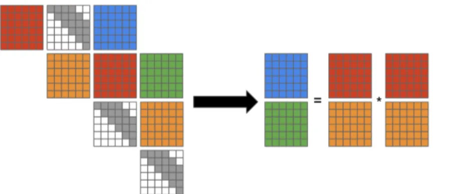
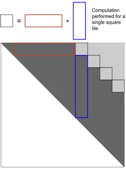
The dependencies of BPMax allow this part of the computation to be performed on all matrices along a diagonal in the 4D table in parallel before advancing to the next diagonal. Therefore, the main need for BPMax is a library of multiple pairs of tropical banded matrix products. We have designed a GPU library call to pairwise multiply two columns of matrices and store the results in a third column, depicted in Figure 5.2a. One call to the library computes only a partial answer for all matrices along a diagonal, thus in the full implementation of BPMax, there is an outer loop over each diagonal of matrices in the table, and an inner loop which iterates over the required number of library calls. The next iteration of the innermost loop for Figure 5.2a is shown in Figure 5.2b.
In our implementation, matrices along a diagonal are laid out consecutively in memory to support the matrix column multiplication scheme.
(a) The computation performed by one call to the GPU library. (b) The next iteration of the innermost loop to compute full answers for the blue and green matrices.
Figure 5.2: Double reduction library call and computation structure. Matrices along a diagonal are laid out consecutively in memory, making each diagonal a column of matrices. Here answers are being computed for the blue and green matrices with two calls to our GPU library.
5.2
First Approach
The main approach for our banded matrix multiplication library is to optimize for two things: 1. skip unnecessary computations to attain 6x speedup over a square matrix multiplication library and 2. Save memory space. Since answers only need to be computed for the banded portion of the matrices, memory locations outside of this area do not even need to be allocated, and since BPMax has significant memory requirements it is important to do this.
Our first approach was to apply affine mappings to the 4D table to save space. The innermost mapping below is similar to the memory saving techniques used in other strategies for banded matrix computations. We applied the following mapping to the outermost dimensions in the table which shifts each matrix down in the grid, and also has the effect of making all matrices along a diagonal become linear in memory where previously all matrices along a row were.
And the innermost indexes are shifted to the left.
i2, j2 7→ i2, i2− j2 (5.2)
After applying these mappings, the dimensions of the grid of matrices in the 4D table is reduced fromN ×N to N ∗N window and the dimensions of each individual matrix is reduced from M ×M toM ∗M window. The memory savings from these mappings are significant. For a problem size N = 400, M = 400, N window = 128 and M window = 128, memory is reduced from 102 GB to 10.5 GB. On the computation side, we skip iterations at the thread block level, but not the individual thread level. The specific way we skipped loop iteration at the thread block level will be explained in more detail in the following subsections because the same strategy was used for our optimal version.
The first version of the library did see a speedup over the square matrix multiplication library since it performs less operations, however it fell quite short of reaching machine peak operations per second, or reaching the 6x speedup over the square library we were hoping for. The reason for this library’s shortcomings is due to the memory mappings we introduced. Because some cells are shifted out of the matrix from these mappings, it introduces thread divergence when loading values into shared memory in the matrix multiplication algorithm. There is no thread divergence at the computation level, but at the level of loading values into a faster, shared memory, we must pad values with the max-plus semiring additive identity if the value the thread should load was actually shifted out from the memory transformations.
5.3
Improved Banded Library
The first version of our library was efficient in terms of memory savings, however it was bottle necked by thread divergence. Therefore, we sought to allocate the minimum amount of memory possible while avoiding thread divergence with memory loads, and at the computation level. For this strategy, memory is allocated based on the configuration of thread blocks that are launched
when we call our GPU library, and rather than allocating a regular 2D structure like a typical matrix, the matrix is allocated similar to a jagged array, and linearly in memory.
5.3.1
Banded Matrix Memory Layout
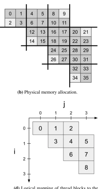
Rather than the standard row major memory layout for a matrix, we organize the memory so all the values a particular thread block will compute an answer for are laid out consecutively in memory. This memory layout has been explored previously by Park et al. [31] where they propose a matrix multiplication memory layout based on the tile size used in a CPU implementation. A depiction of how the thread blocks are mapped to the matrix is given in Figure 5.3a, and the memory allocation based on the thread blocks is shown in Figure 5.3b. If any of the memory locations in the banded portion of the matrix fall within a tile, we allocate the entire tile. This means there will be some tiles which contain both memory locations that need answers computed and some that don’t, and for these tiles on the edge of the band, we initialize the unnecessary cells to the max-plus semiring additive identity, similar to the padding and shifting strategy. The blocks of memory are allocated linearly in memory, like a jagged array, and since each row of thread blocks may have a different number of elements, we must come up with a non-affine function that maps a linear tile address to a 2D address in the matrix.
5.4
Library Modifications
Our original library (see sec. 4.2) launched a 2D grid of thread blocks for each matrix multi-plication instance. In the banded version we instead launch a 1D array corresponding to the exact number of blocks needed as a 2D grid would be wasteful: some of the thread blocks in a 2D grid would be mapped to regions of the matrix where there is no work to do and immediately return. Figure 5.3c shows the linear array of blocks, and Figure 5.3d shows how the thread blocks should be logically mapped to the upper banded matrix. For matrix multiplicationC = A ∗ B, any given tile will start its computation by accumulating the tile in the same row on the diagonal from A with the same tile as its own coordinates from B, thereby skipping most of the redundant work
(a) Thread block data layout. (b) Physical memory allocation.
(c) Thread block arrangement at program run time.
(d) Logical mapping of thread blocks to the data structure.
Figure 5.3: Memory allocation scheme used in our banded matrix library, and how thread blocks are mapped to the matrix.
that square matrix multiplication would do. For example thread block 5 in Figure 5.3d would load the values contained in thread block 3 fromA and thread block 5 from B, perform a partial accu-mulation, then load 4 and 7, then 5 and 8, and accumulate the final answers forC. Thread block 4 would only need to perform the multiplication and accumulation of blocks 3 and 4, then 4 and 6. Therefore, there is a workload imbalance between thread block 5 and thread block 4, but the workload imbalance at the individual thread level is eliminated.
The problem is all the threads in a thread block only know their linear thread block address: all threads in thread block 0 know they are in thread block 0 and so on. In a square matrix size n × n, since the number of elements on any given row is the same, the mapping from a 1D address to the row and column for that address is simple. The row for an entry at linear memory location p is p/n, and the column is given by p%n. For the new banded matrix memory allocation, there is a different number of elements on each row, so the mapping from a 1D address to a 2D address requires a quadratic function.
5.5
Mapping Linear Addresses
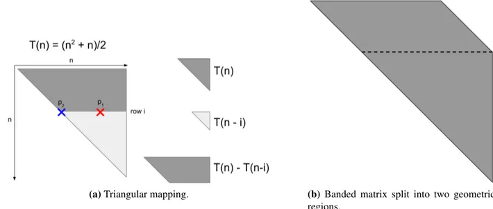
To compute the mapping from a 1D address to a 2D address, we first define a function that returns the number of memory addresses in an upper triangular matrix. The number of elements along the first diagonal in ann × n matrix is n, and each successive diagonal has one less element than the previous. We can represent the number of elements in the entire triangular matrix as the function T (n) = n−1 X i=0 n − i = (n2+ n)/2
Consider computing the address for pointp1 in Figure 5.4, marked by the red X. In this figure point p2, marked by the blue X, is the first point on the same row as p1. If p1 is on row i, then the number of elements belowp1 is a triangular region given by T (n − i). Knowing this, we can compute the addressp2 = T (n) − T (n − i). This expression is simplified to i2− (2 ∗ n + 1) ∗ i + 2 ∗ p1 = 0. Sincep1 and n are known, the quadratic equation can be solved for i to obtain the row that both p1 andp2 are on.
p2 is then at index i, i since it is on the diagonal. The distance between p1 and p2 is simply p1 − p2, so the column index of p1 is i + (p1 − p2). Therefore, all threads in a thread block can compute the 2D index corresponding to the sub-patch of the matrix they are responsible for, and determine which patches of the matrix need to be accumulated.
(a) Triangular mapping. (b) Banded matrix split into two geometric
regions.
Figure 5.4: Algorithm for computing the row and column of a point, given only the linear location of that point in memory and the dimensions of the matrix.
The algorithm just described will only work for triangular matrices. To extend it to banded matrices, we make a simple modification. A banded matrix can be split into two regions as depicted in Figure 5.4b where the upper region is a parallelogram and the lower region is a triangle. For a window size w, which controls the thickness of the band, The triangular region starts at row n − w. The number of elements in the parallelogram region is then (n − w) ∗ w, and the triangular region has dimensionsw × w. In the non-triangular region, the row for a point p is p/width, and the column is i + p%width. Therefore, if the index to be mapped is less than (n − w) ∗ w, we use the parallelogram method just described to calculate the 2D coordinates, otherwise we use the algorithm for the triangular region.
Once the threads in a block have been mapped to a region of the matrix, they no longer have to use the expensive quadratic lookup function which involves a square root. Since memory within a
block is laid out consecutively, coordinates local to a thread block are simple to calculate. Extensive performance results for the optimized banded matrix multiplication library are given in Chapter 7.
5.6
Correctness considerations
Max-plus matrix multiplication is more forgiving than standard multiply-add matrix multipli-cation in terms of yielding a correct answer in the presence of a bug. As long as the largest two values from a particular row of A and column of B are added and have the max operation run on them, the answer will be correct for that particular cell in the C matrix. Missing values or perform-ing extra computations does not affect the answer as long as the maximum value is considered. In multiply-add matrix multiplication, if an extra value is added to a result or a value is missed, the answer is incorrect. This means the potential for a bug to be introduced in tropical matrix multi-plication is much higher if care is not taken to construct proper test cases. To ensure correctness, we developed a test function for our matrix library where the largest value in either input matrix is varied between each location in each matrix. We first make the element at row 0 column 0 in A the largest, run our matrix routine and verify correctness of the answer, then move the largest value to the next column in A and repeat until the value has been varied between all possible positions in A and B. Doing so we can be more sure our GPU library is not missing any cells when computing or doing extra computations it is not supposed to do.
Chapter 6
BPMax: The Remaining Terms
The double max reduction in the recurrence equation is capable of being applied to all outer matrices along a diagonal in the table in parallel, but this results in partial answers for those cells. Thus after applying the matrix multiplication library call to matrices along an outer diagonal, there must be a patch up phase which computes the full answers.H1, H2, H3, and H4all perform reduc-tion operareduc-tions, using values from the F table, and two different tables which maintain informareduc-tion about single strand folding for the input RNA molecules,S(1) andS(2). The F table values for the reductions inH3 andH4 all come from matrices outside of the one being evaluated, so it is legal to perform the reduction for each cell in each matrix along a diagonal in parallel, a similar schedule to the double reduction computation. However, the reductions forH1 andH2use values from within the same matrix since the reduction is over thei2 andj2 dimensions, and because of this it isn’t legal to evaluate them for all points within a matrix in parallel. FromH1, each point in the F table requires the value immediately to the left of it to be completed, and fromH2, each point requires the one immediately below it. The computation pattern forH1andH2 very closely follows that of single strand RNA folding.
6.1
Optimizations
Since the H1. . . H4 terms are all reductions, the arithmetic intensity of these computations is just one operation per element loaded, and thus they are memory bound rather than compute bound. The choice of which RNA strand to make the outermost dimensions in the 4D table and which to make the innermost dimensions affects the operations required for these terms as well. In the data set we present in the experimental results chapter, BPMax is run when the first RNA is size 19-23 nucleotides, and the second RNA varies from 50 - 40,000 nucleotides. There are two choices for this data set, to make a large grid of very small matrices, or to make a small grid of very large matrices. Since the double reduction term is performing matrix multiplication, it will typically
(a) Strategy used by Rizk et al. proceeds diagonal by diagonal, evaluating square tiles in advance followed by a patch up phase over a small trapezoidal region, where the next tiled computation would begin.
(b) Strategy used by Li et al. computes full answers for all cells surrounding the square tiles first before performing the tiled com-putation, the patch up phase operates on the square tiles only, not for all points along the diagonal. After the square tiles are patch up, the next tile phase begins.
Figure 6.1: Algorithm comparing different methods for computing single strand folding. Our strategy is similar to (b), but evaluates multiple instances in parallel.
achieve better performance doing a small number of very large matrix multiplications rather than a large number of very small matrix multiplications. This has an impact on the performance of theH functions becauseH1andH2have complexityO(N2M3) and H3, H4have complexityO(N3M2). When the grid is small and matrices are large, it is more important to optimize H1 and H2, and more important to optimizeH3andH4 when the grid is large and matrices are small.
6.2
H1 and H2
Our optimization approach for the H1 and H2 functions follows the work done by Rizk et al. and Li et al. for tiling single strand folding [9, 10]. Rizk observed that most of the operations for a tile of memory locations can be computed in advance with a computation that essentially performs max-plus matrix multiplication, followed by a patch up phase. Rizk split the reduction for each point into three parts, where the middle part of the reduction could be expressed as matrix multiplication. Li et al. modified how the patch up phase works to get a marginal improvement, both methods are illustrated is Figure 6.1. Our algorithm is similar to Li et al., except we perform multiple simultaneous instances of the single strand folding algorithm on the GPU, and in addition, their version had each GPU thread computing a single value in the table during the patch up phase, but this is parameterized in our version, a thread may evaluate multiple values in the patch up phase. We still mostly go diagonal-by-diagonal over the matrix, but now most of the computation has exploited data re-use.
6.3
H3 and H4
The H3 and H4 functions do not have any intra-matrix dependency, so we can evaluate all points in parallel and do not need to go diagonal-by-diagonal. Therefore,H3, H4are implemented in BPMax as an optimized GPU reduction. A further improvement could speed these terms up more by fusing them with the double reduction. Since all the values needed byH3 andH4 from theF table come from matrices below and to the left of the matrix being evaluated, at some point in the double reduction those values will be read in. However, H3 and H4 are not a bottleneck
for the data set we evaluated on. There is no host side synchronization overhead likeH1 andH2 because all points are evaluated in parallel, and since we use a small grid of large matrices, the work required forH3andH4 is an order of magnitude less thanH1andH2. Even after optimizing H1 and H2, those terms still contribute to more total run time than H3 and H4, so we did not explore fusing with the double reduction since it would have provided negligible speedup.
Chapter 7
Experimental Results
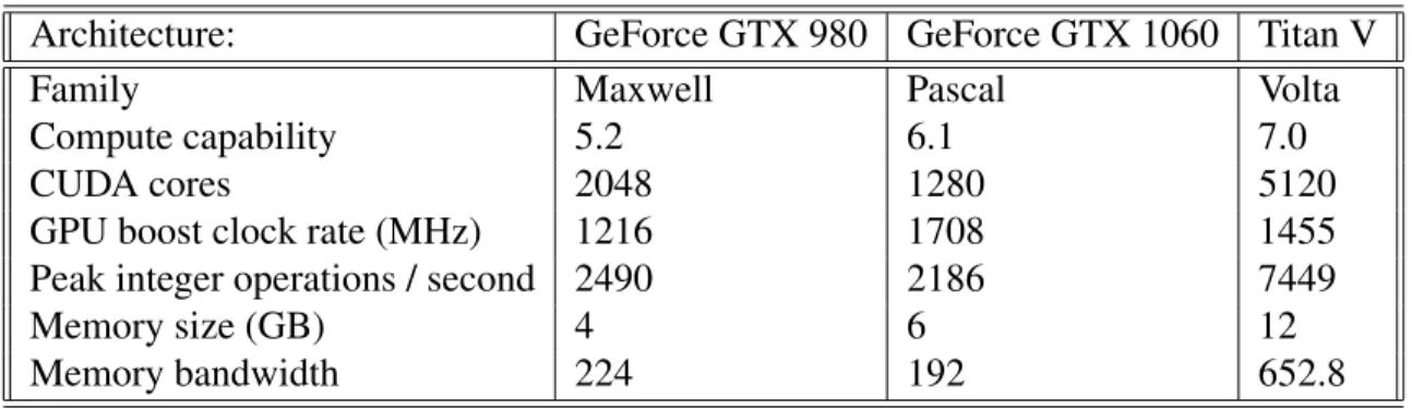
Performance of the various library calls is evaluated across three different GPU architectures. A summary of each card is given in Table 7.1. In this chapter, we first describe our bench marking process and what metric we sought to optimize, then describe the performance of the tropical ma-trix multiplication library first when the window size is unrestricted, then with a restricted window size, then discuss the performance of the H1. . . H4 functions. We compare the performance of our banded matrix multiplication library to a library that performs square tropical matrix multi-plication, developed by Ghalsasi [27], which attains machine peak performance, and use this to demonstrate the need for the banded library.
Table 7.1: Technical specifications of GPUs used in experiments.
Architecture: GeForce GTX 980 GeForce GTX 1060 Titan V
Family Maxwell Pascal Volta
Compute capability 5.2 6.1 7.0
CUDA cores 2048 1280 5120
GPU boost clock rate (MHz) 1216 1708 1455
Peak integer operations / second 2490 2186 7449
Memory size (GB) 4 6 12
Memory bandwidth 224 192 652.8
7.1
Performance Benchmark Considerations
When considering the performance of the banded matrix multiplication library, we develop a term called effective work. Effective work describes the minimum work required for a banded matrix multiplication. The total operations required for square matrix multiplication is2 ∗ N3, and the total operations required by triangular matrix multiplication is 1/3 ∗ N3. When the window
size is reduced, the upper triangular region of the matrix, dimensions (N − W )2, is subtracted from the work, so the total work required is 1/3(N3 − (N3 − W3)). Effective operations per second is then 1/3(N3 − (N3 − W3))/runtime. We use this term to demonstrate the need for developing a banded matrix multiplication library. No existing library performs the multiplication of two banded matrices, so if we plug a square library into BPMax which attains machine peak performance in terms of operations per second, the effective work done by the square library will be poor, because it is doing many redundant operations. The banded library we developed still does some redundant or useless operations, and attains close to machine peak operations per second as the square library does, but more importantly, it attains close to machine peak effective operations per second as well. Ultimately, the metric we want to optimize is run time, and since the libraries perform useless operations, if we try to maximize total operations per second as is typically the goal in high performance computing applications, this does not necessarily result in the minimum run time. Since we pad the matrix out to the next multiple of the thread block dimensions, there are cases where padding it out further would increase total operations per second, but reduce effective operations per second. Maximizing effective operations per second will result in minimum run time for this library.
7.2
Triangular Matrix Performance
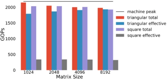
Figure 7.1 gives a comparison of total operations per second achieved by the banded library and a square matrix multiplication library when the window is unrestricted. Each trial was ran with a column of 20 matrices. The black horizontal line shows the machine peak performance, 2186 GOPs for the GTX 1060. When considering total ops / second by the square and banded library, both achieve 90-95% of machine peak. Both libraries are doing redundant work, but the banded library is optimized to do far less redundant work than the square library. The effective performance for the banded library is almost the same as its overall performance, but the effective work for the square library is 1/6 of its overall performance. We attain up to 88.5% effective peak performance for the banded library, while the square library delivers 17.5% of peak effective
performance. Figure 7.2 demonstrates the library is portable across architectures, reaching 80-90% of effective peak on each. To obtain peak performance, a script was used to tune the library to the best parameters for each problem size.
Figure 7.1: Total work and effective work comparison of the banded matrix library and the square library. Results were collected on a GTX 1060. The window size of each matrix is unrestricted, and the library was called with columns of 20 matrices.
7.3
Varying the Matrix Size and GPU Parameters
Figure 7.1 gives performance for problem sizes that perform well for matrix multiplication, when the matrix dimensions are powers of 2. All GPU matrix multiplication libraries typically reach peak performance for these specific problem sizes. However, the input RNAs can ultimately be any size, so it is important to benchmark and tune performance across a broader range of inputs. The double reduction library call is parameterized by how many threads per block are used, how many elements in the matrix each thread should compute, the size of shared memory for each thread block, as well as a few other variables, and theH1. . . H4functions have several parameters as well. Tuning all of these parameters gives different performance for different problem sizes, but the difficulty is the search space for optimal parameters for any given input size is so large, it takes much longer to search for the optimal parameters then run the program, than it does to run the program with sub-optimal parameters. Therefore, it is important to study how the program
Figure 7.2: Banded library performance across three GPU architectures. For each card, 80-90% of effective machine peak is reached.
performs across a broad range of input sizes and figure out what good parameters are in general for various inputs, so we can set the run time parameters to good enough values before performing a large experiment. For this study, we created a script that modifies all the parameters in each GPU library call, re-compiles the program and collects performance data. This script alone takes over one day to run when the matrix size is varied from 50 up to 20,000, and we used the data from this script to determine what good general parameters are. When the input RNAs are smaller, performance does not matter as much because the run time for the program is under one second anyways, but for large inputs, the run time quickly increases, so we chose to select values for our experiment that give better results on large inputs, knowing the contribution to the total run time for smaller RNAs across a large experiment does not matter as much. Figure 7.4 shows performance for the double reduction call on matrices anywhere from 500 × 500 - 6000 × 6000, for two different sets of run time parameters we found to perform well. For smaller matrix sizes, the 8 × 8 thread version performs better, and as the matrix size increases the 16 × 16 thread version overtakes it in terms of performance. The sharp jumps illustrate how sensitive the performance is with respect to the run time parameters for small matrices, but as the matrix size grows, the performance is more stable.
Figure 7.4: Banded matrix library effective performance with varying matrix sizes and number of threads. Experiment ran on a Titan V GPU with columns of 23 matrices.
7.4
Banded Matrix Performance
Decreasing the window size reduces the effective operations per second of both libraries. In a more extreme case where the window size is reduced to 128, the problem is more similar to multiplying very tall, skinny matrices. Depending on how small the window size is, it can make the problem memory bound rather than compute bound [32]. Furthermore since there is a work-load imbalance in banded matrix multiplication, when the window size is reduced it removes the cells that require the most operations from the computation. These two changes result in poorer utilization of GPU resources. When the window size is reduced down to 128, the iteration space of the multiplication becomes much smaller and ultimately each thread block has less work to do for each patch of shared memory, and performance drops. If the library is called for a matrix size 8192×8192 with a window of 128, we should expect performance more similar to the performance of a smaller matrix multiplication on a GPU rather than a large one. Figure 7.5 shows the perfor-mance of the library for varying matrix sizes with a window size of only 128. The library attains 60% of machine peak for total operations per second, and 32% of peak performance for effective operations per second. The total operations per second of the square library on banded matrices compared to triangular matrices is the same because it is not optimized for banded matrices, and the effective work drops to less than 1% of machine peak for larger matrices, clearly illustrating the benefits of the banded library for this specialized matrix routine.
7.5
Varying the Window Size
To see how the window size affects performance for different thread configurations, the window size for a 2048× 2048 matrix was varied from 128 to 2048 and ran with a version of the program using 8 × 8 threads, and 16 × 16 threads. Results are presented in Figure 7.6. The results here seem to follow the results when the matrix size was varied. As the size of the matrix increases, and the window size approaches its full length, larger thread blocks work better, and for smaller sizes smaller ones do.
Figure 7.5: Total work and effective work comparison of the banded matrix library and the square library. Results were collected on a GTX 1060. The window size of each matrix is 128, and the library was called with columns of 20 matrices.
7.6
Performance of
H
1through
H
4Figure 7.7 shows the performance of the H1 library call for varying matrix sizes. The perfor-mance of H2 is identical, since the only difference is the tables the columns and rows are read from is swapped.
Figure 7.7: H1, H2 Performance. Experiment ran on a GTX 1060 with 20 matrix per column, no window
restriction.
We achieve up to 33% of machine peak in Figure 7.7 which is comparable to other GPU libraries in the literature for single strand folding [9, 10]. The tiled matrix multiplication portion of this algorithm is very efficient and achieves near machine peak performance, however the patch up phase is bottle necked by memory bandwidth. A typical problem size from the data set presented in the following section ranges in size from 50-40,000 nucleotides, and the grid of matrices is around 20 × 20. For a matrix 10,000 × 10,000 from this data set, during the patch up phase around 200,000 very small reduction computations would be launched. Small reduction problems are not a good match computationally for what GPUs excel at. GPUs excel at very large problems where the computation is regular, meaning no workload imbalance. In the patch up phase, there is many instances of very small reductions, and each reduction has a different amount of work, which is dependent on its local coordinates within a thread block.
The H3 and H4 functions do not have the complex dependencies the H1 and H2 functions have, they are implemented on all cells in a matrix in parallel as a reduction. Since we have a choice of which RNA molecule corresponds to the grid dimensions, we can make the smaller of the two molecules the grid of matrices which means the H3 and H4 functions are much faster and are not bottlenecks in the current implementation of BPMax GPU. Therefore, we don’t present extensive performance results for these functions, the focus of our optimizations are the double reduction and the H1 and H2 functions.
Chapter 8
SARS-CoV Data Set
Three small viral RNAs (svRNAS) of interest were identified in the SARS-CoV genome [33]. SARS-CoV-2, the virus that caused COVID-19, is from the same family as SARS-CoV. Boroojeny and Chitsaz recently reported potential orthologs of the three svRNAs, from SARS-CoV, present in the SARS-CoV-2 genome [34]. Boroojeny and Chitsaz also processed a data set of 32,000 RNAs transcribed in the human body to remove the intron regions of each. We then ran BPMax for each svRNA against all 32,000 processed RNAs to identify potential target genes of the svRNAs. The following benchmarks were obtained using problem sizes from that data set. The three svRNA orthologs are sizes 18, 22 and 23 nucleotides, and the processed RNAs from the human genome range anywhere from 41 to 205,012 nucleotides. The Titan V GPUs available in our department have 12GB of memory, and because of this memory constraint, we removed the largest 14 RNAs from the data set. The largest RNAs we ran BPMax with was 40,000 nucleotides, against the 23 nucleotide svRNA, which makes the 4D dynamic programming table have a memory footprint of around 11GB.
The results of this study are still being analyzed, so here we present performance results without analysis of potential biological findings, if any, from the data set.
Chapter 9
Full BPMax Performance
Figure 9.1 gives performance in effective operations per second when the first RNA molecule is 23 nucleotides and the second ranges from 1000 - 20,000, for both the GPU program and the original implementation of BPMax. When computing effective operations, only the run time from the computation is considered, not including data transfer times to/from the GPU. The first RNA is not windowed, and the second is set to a window of size 128. The GPU version is run on the fastest GPU available in the computer science department at CSU, the Titan V, and the CPU version is ran on the fastest CPU available at CSU, an Intel Xeon E-2278G, which clocks at 5 GHz/second, and has 8 hyper-threaded cores. As the input size increases, the giga-operations per second (GOPs) delivered by the GPU stays nearly constant. On the CPU, the GOPs decreases as the problem size increases, from 1.1 GOPs to .11 GOPs.
Figure 9.2 gives end to end run time for BPMax, including data transfer times to and from the GPU. An RNA of size 20,000 takes 4.79 seconds to process on the GPU, and 3056 seconds to process on the CPU implementation. The entire data set of 32,000 RNAs ran with a single svRNA can be processed in about one day on department machines, and a back of the envelope calculation shows the original CPU implementation would require on the order of 3 months of execution time on a single machine, so the computation would have to be distributed to several hundred machines to achieve the results at the same speed of a single GPU.
9.1
Bottleneck Analysis
In Figure 9.1, BPMax is not reaching anywhere near the machine peak performance of 7449 GOPs, the best performance is around 12% of theoretical peak. For the input RNAs size 23 and 1,000, and a window size of 128, the average run time is around .58 seconds. To figure out the contribution of the run time with respect to each term, BPMax was ran with all terms besides a single one removed, and doing so revealed the average run time for the H1, H2 functions is
Figure 9.1: Performance of full BPMax, original CPU implementation and GPU implementation. RNA 1 is 23 nucleotides and RNA 2 is varying size with a window of 128. Experiments ran on a Titan V GPU, and an Intel Xeon E-2278G CPU.
Figure 9.2: GPU run time showing computation time and end to end execution time which includes data transfers to and from the GPU. RNA 1 is 23 nucleotides and RNA 2 is varying size with a window of 128. Experiments ran on a Titan V GPU
Figure 9.3: CPU run time on a semi-log plot. RNA 1 is 23 nucleotides and RNA 2 is varying size with a window of 128. Experiments ran on an Intel Xeon E-2278G CPU.
nearly 3× longer than the average run time for the double reduction, despite requiring an order of magnitude less work.
When only the double reduction is run, the programs attain around 730 GOPs per second, which matches the expected performance based on Figure 7.5 for matrix size 1000 and window 128. For the same input RNAs with the window unrestricted, the program attains near machine peak performance if only the double max reduction is run, matching the performance expectation from Figure 7.1. When runningH1, H2 only with a window of 128, the program attains only 25 GOPs, much less than the results presented in Figure 7.7, because the performance drops when the window is restricted just like the matrix multiplication library. The patch up phase ofH1, H2 is severely bandwidth bound, and prevents BPMax from reaching peak performance. In Rizk’s work, around 23% of machine peak was attained, and it was noted in the conclusion it would be difficult to improve this kernel further. Our implementation faces the same limitations as the implementation in their work, with the added difficulties of the windowing which their work did not consider.
Chapter 10
Conclusion and future work
In this paper we provided the first optimized GPU implementation of BPMax, a recently pro-posed algorithm for predicting RNA-RNA interactions. Previous implementations exploit a naive parallelization strategy which makes the programs severely bandwidth bound, and unable to reach even 1% of theoretical machine peak. We showed how by reordering operations and transforming the dynamic programming table we can express the innermost three loops of BPMax (and other RRI algorithms), as an instance of banded matrix multiplication using max-plus operations. We provide the first library performing banded-banded matrix multiplication, and calibrate it to attain near machine peak performance. This allows us to more efficiently exploit tiling and other proper-ties to attain significant speedup, and ultimately perform a study of three small viral RNAs which are hypothesized to be relevant to COVID-19.
This optimization of BPMax is just the first step, and there is much future work on the topic of RNA-RNA interaction. Current ongoing work is focusing on providing an optimized CPU implementation of BPMax. By applying the same operation reordering techniques and exploiting multi-threading on a state of the art processor, the CPU implementation could be competitive with the GPU. Perhaps more importantly, a CPU implementation would not have such severe memory constraints which currently limit the GPU version. Machines with one or more terabytes of RAM are exceedingly common and are capable of processing much longer sequences.
Another open problem is a multi-GPU parallelization of BPMax capable of handling larger sequences. This is one way of overcoming the memory size constraints, but because the inter-GPU communication over PCI is significantly slower than memory transfers on a single inter-GPU, we would need a completely different parallelization strategy, since a straightforward extension of the algorithms we used in this paper is unlikely to be effective.
Taking the lessons we learn from BPMax, we will then focus on optimizing more complex RRI programs which incorporate thermodynamic information. BPPart computes the partition function
and is a constant factor of 10 higher in run-time complexity and memory requirements. BPPart also fills up a 4D dynamic programming table, and follows a very similar computation pattern to BPMax, so the optimization techniques will be similar but must deal with the added complexity of computing the partition function. Ultimately, a longer term goal is the acceleration of piRNA, the most complex RRI algorithm.
Bibliography
[1] Stefanie Mortimer, Mary Kidwell, and Jennifer Doudna. Insights into RNA Structure and Function from Genome-Wide Studies. Nat. Rev. Genet., 15:469–479, July 2014.
[2] Mirko Ledda and Sharon Aviran. Patterna: Transcriptome-wide Search for Functional RNA Elements via Structural Data Signatures. Genome Biol., 19:28, March 2018.
[3] Hamidreza Chitsaz, Raheleh Salari, S. Cenk Sahinalp, and Rolf Backofen. A partition func-tion algorithm for interacting nucleic acid strands. Bioinformatics, 25:365–373, May 2009. [4] Dmitri Davidovich Pervouchine. IRIS: Intermolecular RNA Interaction Search. Genome
Inform., 15:92–101, January 2004.
[5] Fenix W. D. Huang, Jing Qin, Christian M. Reidys, and Peter F. Stadler. Partition func-tion and base pairing probabilities for RNA-RNA interacfunc-tion predicfunc-tion. Bioinformatics, 25(20):2646–2654, 2009.
[6] Ali Ebrahimpour-Boroojeny, Sanjay Rajopadhye, and Hamidreza Chitsaz. BPPart and BP-Max: RNA-RNA Interaction Partition Function and Structure Prediction for the Base Pair Counting Model, 2020.
[7] Ruth Nussinov, George Pieczenik, Jerrold Griggs, and Daniel Kleitman. Algorithms for Loop Matching. J. Appl. Math., 35:68–82, June 1978.
[8] Michael Zuker and Patrick Stiegler. Optimal computer folding of large RNA sequences using thermodynamics and auxiliary information. Nucleic Acids Res., 9:133–148, January 1981. [9] Guillaume Rizk, Dominique Lavenier, and Sanjay Rajopadhye. GPU Accelerated RNA
Fold-ing Algorithm, chapter 14, pages 199–210. Morgan Kaufmann, 2011.
[10] Junjie Li, Sanjay Ranka, and Sartaj Sahni. Multicore and GPU Algorithms for Nussinov RNA Folding. BMC Bioinformatics, 15, July 2014.
[11] M Shel Swenson, Joshua Anderson, Andrew Ash, Prashant Gaurav, Zsuzsanna Sukosd, David Bader, Stephen Harvey, and Christine Heitsch. GTfold: Enabling Parallel RNA Secondary Structure Prediction on multi-core Desktops. BMC Res. Notes, 5, July 2012.
[12] Balaji Venkatachalam, Dan Gusfield, and Yelena Frid. Faster Algorithms for RNA-folding using the Four-Russians method. Algorithms Mol. Biol., 9, March 2014.
[13] Dar-Jen Chang, Christopher Kimmer, and Ming Ouyang. Accelerating the Nussinov RNA folding algorithm with CUDA/GPU. In ISSPIT ’10: Proceedings of the the 10th IEEE
Inter-national Symposium on Signal Processing and Information Technology, 2010.
[14] Saeed Maleki, Madanlal Musuvathi, and Todd Mytkowicz. Low-Rank Methods for Paral-lelizing Dynamic Programming Algorithms. ACM Transactions on Parallel Computing, 2, February 2016.
[15] Aydın Buluç, John R. Gilbert, and Ceren Budak. Solving path problems on the GPU. Parallel
Computing, 36:241–253, June 2010.
[16] Leslie G. Valiant. General Context-Free Recognition in Less than Cubic Time. Journal of
Computer and System Sciences, 10:308–315, April 1975.
[17] Yasubumi Sakakibara, Michael Brown, Richard Hughey, I.Saira Mian, Kimmen Sjolander, Rebecca C.Underwood, and David Haussler. Stochastic context-free grammars for tRNA modeling. Nucleic Acids Res., 22:5112–5120, November 1994.
[18] James WJ Anderson, Paula Tataru, Joe Staines, Jotun Hein, and Rune Lyngsø. Evolving stochastic context–free grammars for RNA secondary structure prediction. BMC
Bioinfor-matics, 13:308–315, May 2012.
[19] Shay Zakov, Dekel Tsur, and Michal Ziv-Ukelson. Reducing the worst case running times of a family of RNA and CFG problems, using Valiant’s approach. Algorithms Mol. Biol., 6, August 2011.