2009:33 Workshop on spent fuel performance, radionuclide chemistry and geosphere transport parameters, Lidingö 2008: Overview and evaluation of recent SKB procedures

Workshop on spent fuel performance,

radionuclide chemistry and geosphere

transport parameters

Lidingö 2008: Overview and evaluation of recent SKB procedures

Research

2009:33

Title: Workshop on spent fuel performance, radionuclide chemistry and geosphere transport parameters, Lidingö 2008: Overview and evaluation of recent SKB procedures.

Report number: 2009:33.

Authors: Günther Meinrath, Mike Stenhouse, Paul Brown, Christian Ekberg, Christophe Jégou and Heino Nitsche.

Date: August 2009.

This report concerns a study which has been conducted for the Swe-dish Radiation Safety Authority, SSM. The conclusions and viewpoints presented in the report are those of the authors and do not necessarily coincide with those of the SSM.

SSM perspective Background

The safety assessment for disposal of spent nuclear fuel canister in the Swedish bedrock should thoroughly address the time period after a con-tainment failure. Such a failure could be expected as a result of corrosion damage or mechanical failure due to rock movement. This report mainly covers some issues connected to parameters used for radionuclide transport calculations in the areas of spent fuel performance (for fuel in contact with groundwater), radionuclide chemistry, and sorption and geosphere trans-port parameters. Some examples of topics that are elaborated in some detail include statistical treatment of measurement data (for sorption measure-ments), handling of uncertainties in speciation calculations, use of triangu-lar distributions in safety assessment and physical processes in connection with spent fuel aging. The results emerged from discussions among interna-tional experts at a workshop, Lidingö, Sweden, May 2008.

Purpose of Project

The purpose of this work is providing an overview of ongoing work within the Swedish Nuclear Fuel and Waste Management Co. (SKB), to provide ideas and suggestions for methodology development and to develop review capability within the SSM.

Results

The authors conclude that SKB’s treatment of uncertainty in speciation calculations has improved, but that additional efforts in the area of er-ror propagation are recommended. In efforts to condense the scope of utilised thermodynamic databases, the authors recommend that exclu-sion criteria should be explicitly stated. In the area of sorption, there is a need for more thorough analysis of errors in order to establish uncer-tainty ranges. The most essential improvements concern dose-limiting nuclides (e.g. Ra-226). Triangular distributions are often featured in SKB safety assessment, but it is not clear that the use of such distributions is based on a firm understanding of its properties. Regarding fuel perfor-mance, while safety assessment parameters are supported by measure-ment data there is still a need for better understanding of the detailed reaction mechanisms and aging effects over very long time-scales.

Future work

In the future, SSM need to develop and extend the knowledge basis for assessment of spent fuel and radionuclide retardation processes. There may also be a need to further expand the capability to conduct indepen-dent speciation calculations.

Project Information

Project manager: Bo Strömberg Project reference: SSM 2008/903

Content

1. Introduction...3

2. SKB/SKI/SSI workshop ...6

3. Spent Fuel Dissolution – Current Issues and Recent Research ...9

3.1 Instant Release Fraction ...9

3.1.1 Diffusion process in spent fuel – new data and conclusions ...10

3.1.2 Fate of helium in spent fuel rods...11

3.2 Matrix Alteration ...11

3.2.1 Influence of hydrogen ...11

3.2.2 Conclusions regarding spent fuel matrix alteration.12 3.2.3 General considerations on the Rapid Release Fraction used for PA...12

3.3 Overall Conclusions on Spent Fuel Source Term ...13

4. Geochemical Database and Solubility Model...14

4.1 Modelling Approach ...14

4.2 Radium Database and Solubility Limits...17

4.3 Uranium Database and Solubility Limits...18

5. Note on Some Relevant Properties of Swedish Groundwaters...20

5.1 Swedish Groundwater Data: EH-pH...20

5.2 Carbonate in Groundwaters...25

5.3 Swedish Groundwaters: pH vs. lg [HCO3-] ...28

6. Data Reliability and GUM-Compliant Uncertainty Assessment of Sorption Data ...29

6.1 Sorption...29

6.1.1 Process ...29

6.1.2 Uncertainty Analysis of Experimental Sorption Data 30 6.2 Assessing a Sorption Coefficient Kd According to the GUM Convention...34

6.2.1 Step 1: Specify quantity being evaluated ...34

6.2.2 Step 2: Identify possible influences ...35

6.2.3 Step 3: Identifying relevant influences...35

6.2.4 Step 4: Quantify uncertainty...39

7. Data Variability and the Use of the Triangular Distribution...42

7.1 Context...42

7.2 Issues Concerning the Use of the Triangular Distribution...42

7.3 Conclusions – Remaining Questions...45

8. Transport Properties in the Geosphere: Additional Input from SKB...47

8.1 SKB Responses to Issues Raised ...47

9. Summary...52

References...55

Appendix A: The Role of Microbiological Systems in Natural Aqueous Environments ...59

Annex A: Swedish groundwater data (Bath, 2008) ...62

Appendix B: Good Laboratory Practice (GLP) and Guide to the Expression of Uncertainty in Measurement (GUM) ...65

B.1 Introduction ...65

Annex B: Extracts from “Development of Methodology for

Evaluation of Long-term Safety Aspects of Organic Cement Paste

Components” by Andersson et al., (2008)...68

Appendix C: Properties of the Triangular Distribution ...74

C.1 Introduction ...74

C.2 Characteristics of Triangular Distribution...76

C.3 Alternatives to Triangular Distribution...81

1. Introduction

SR-Can covers the containment phase of the KBS-3 barriers as well as the consequences of releases of radionuclides to the rock and eventually the biosphere (after complete containment within the fuel canisters has partially failed). The 2007 review (Stenhouse et al., 2008) and this follow-on report provide a range of review comments concerning parameters related to spent fuel performance as well as radionuclide chemistry and transport. These parameter values are used in the quantification of consequences due to re-lease of radionuclides from potentially leaking canisters. This report does not cover the modelling approaches for quantification of consequences. Such approaches are discussed elsewhere.

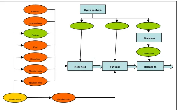
Figure 1 gives an overview of the data used for the consequence assessment in SR-Can. Parameter values contained in the red boxes have been (SKI, 2007; Stenhouse et al., 2008) and are addressed by the authors of this report, while parameters with green boxes are addressed in other contexts, e.g. pa-rameters from the hydrology and biosphere assessment that are addressed in e.g. SSM’s review of the now-completed site investigations. The groundwa-ter chemistry is addressed to a limited extent as a critical input for the devel-opment of a geochemical database and the solubility model used as a basis for estimating radionuclide solubility. In this context, a section is devoted to some relevant properties of Swedish groundwaters.

Figure 1: Overview of the data used for the consequence assessment in

SR-Can. Parameter values contained in the red boxes are addressed in this re-port, while the other boxes are addressed in other contexts of the SR-Can review (figure reproduced from SKB SR-Can TR-06-09, page 400).

Instant release Inventory Migration data Migration data Migration data Canister Fuel Solubilities Groundwater Biosphere Hydro analysis

Near field flow Far field flow Exit points

Landscape

Near field Far field Release to

R

ele

as

The work reported here is intended to complement and extend the review findings reported in SKI Reports 2007:17 (SKI, 2007) and 2008:17 (Sten-house et al., 2008), which cover previous workshops held in 2006 and 2007, respectively, on issues associated with spent fuel dissolution and source term modelling in safety assessment. Topics covered by the review team in these previous reports together with the associated SKB reports include spent fuel performance parameters (Werme et al., 2004, SKB, 2006c), concentration limits in the near field (Duro et al., 2006a) and the supporting thermody-namic database (Duro et al., 2006b), migration parameters in the buffer (Ochs and Talerico, 2004, SKB, 2006d) and far field (Liu et al., 2006, Craw-ford, 2006, SKB, 2006e).

Additional items reported in SKI Report 2008:17 (Stenhouse et al., 2008) included some details in actinide chemistry and in the 4n+2 decay chain, as well as co-precipitation of radionuclides with major element phases. The decision to focus on the latter was based on the observations in SR-Can, that neglecting co-precipitation of Th-230 may be non-conservative, and that accounting for co-precipitation of Ra-226 with Ba may significantly lower calculated doses. Considering the relatively limited resources available for these reviews, some of the issues have been scrutinised only to a rather lim-ited extent. It is therefore recommended that additional research and review resources continue to be devoted to this area over the next few years. Uncertainty and sensitivity analysis have framed much of the review discus-sions over the past three years. An appropriate handling of uncertainties is considered not only important in the context of SR-Site, but also should be apparent in the SKB safety assessment work. In the SSM regulations and guidelines SSM 2008:21 (in 9§ and appendix), it is stated that uncertainties should be discussed and examined in depth when selecting calculation cases, calculation models and parameter values as well as when evaluating calcula-tion results. Thus, a systematic identificacalcula-tion and characterisacalcula-tion of the various sources contributing to uncertainty is necessary. SKB’s approaches for handling uncertainties related to the relevant safety assessment parame-ters were discussed in SKI 2008:17 (Stenhouse et al., 2008).

Sensitivity analysis, also required according to the above-mentioned regula-tion and guidelines, is strongly related to the handling of uncertainties. It is a tool for prioritising the efforts needed in the handling of uncertainties. For example, within the area of spent nuclear fuel and radionuclide chemistry, it is important to ensure the availability of reliable information for those nu-clides that contribute the most to calculated dose within various calculation cases.

SSM experts provided a description of alternative/complementary ap-proaches for uncertainty and sensitivity analyses in SKI 2008:17 (Stenhouse et al., 2008) and this treatment is extended in this report to cover, for exam-ple, a detailed assessment of the uncertainty associated with the estimation of Kd values.

Section 2 of this report briefly discusses SKB’s presentations made at the 2008 Workshop and some highlights from the discussions with SSM and its

consultants at the Workshop, Section 3 discusses recent research being car-ried out in Europe concerning spent fuel dissolution and resultant incorpora-tion of the source term in performance / safety assessment. Secincorpora-tion 4 ad-dresses specific aspects of the geochemical database and modelling approach used by SKB to determine solubility-limiting phases for radium and ura-nium. Section 5 discusses the uncertainties in interpreting groundwater data with particular consideration of the potential effects of microbial systems. Section 6 addresses data reliability from a quality-assurance perspective and examines an internationally-accepted method of evaluating uncertainty, us-ing sorption data as a specific example. Section 7 examines the validity of applying the triangular distribution to account for data variability. Section 8 contains SKB responses to specific questions raised before and during the Workshop on transport properties in the geosphere, specifically concerning measurements of matrix diffusion and sorption-related parameters. Finally, Section 9 provides summary comments.

2. SKB/SKI/SSI workshop

At the SKI-SSI/SKB Workshop in 2008 (May 29), partly in response to pre-vious review comments, SKB and its consultants gave a number of presenta-tions, viz.

 Scenario Analysis - Uncertainty and Sensitivity Analysis (Alan Hedin)

 Radionuclide Migration in the Near Field (Patrik Sellin)  Spent fuel source terms (Kastriot Spahiu)

 Radionuclide solubility limits and thermodynamic data (Lara Duro)

 Radionuclide migration in the Far Field (Jan-Olof Selroos). While the Workshop itself was not part of formal consultations, the above presentations and the discussions that followed gave SKI’s consultants a better understanding of SKB’s approach in the selected areas of the SR-Can assessment. Largely as a result of these presentations and the discussions that ensued, some general comments are provided as bullet points below.

 Scenario analysis: The main (dose-limiting) scenario involves en-hanced corrosion whereby buffer loss (chemical erosion) is the key process. Enhanced corrosion leads to an estimated 9 (out of a total of 6000) canisters failing. As a bounding case, SKB also considered buffer loss immediately, with results similar to the main scenario. While in previous assessments, I-129 was the dominant radionu-clide, the current safety assessment results indicated that Ra-226 is now the key (dose-limiting) radionuclide.

 Radionuclide migration in the near field: SKB noted that tempera-ture is not a concern with regard to radionuclide release because am-bient temperature is reached by the time canisters have failed and radionuclides are released. While Äspö diffusion experiments were not designed for radionuclide transport, they have provided some useful insights into transport in the near field. SKB uses a range of groundwater compositions to allow for mixing waters and bentonite porewater evolution. SKB also noted that the issue of updating the specification for the backfill had still to be resolved, although loss of backfill material does not necessarily lead to higher doses.

 Spent fuel source terms: SKB discussed the experimental work that is being carried out to support spent fuel dissolution rates and ra-dionuclide releases for safety assessment calculations, in particular experiments carried out as a function of burnup, with maximum re-leases observed to occur around 40/45 MWd/kgU. In addition, leaching experiments being carried out by ITU-ENRESA allow comparison of the outer parts of the fuel with the core, with results mainly indicating greater releases from core material (with some ex-peceptions e.g. Tc). There was detailed discussion about the basis for SKB’s instant release fraction (discussed in Section 3).

 Radionuclide solubility limits and thermodynamic data: There was significant discussion about error propagation in the context of solu-bility limits. In this context, the lack of reliable phosphate data, par-ticularly for transuranic elements was also discussed. SKB’s current uncertainty propagation is based on variability in groundwater com-position rather than error propagation through the thermodynamic database. SKB’s objective is to get away from the concept of a ‘ref-erence groundwater’ and rather accommodate ranges of groundwater component concentrations via multiple (~10,000) realisations. Im-portantly, SKB noted that a change in solubilities by 2 orders of magnitude either way does not affect assessment results. In addition, if the buffer erosion scenario continues to dominate exposure dose results, solubilities will play a less important role, although under oxidizing conditions, solubility will be important for Np.

 Radionuclide migration in the far field: SKB discussed its philoso-phy for selecting Kd values - generally, with regard to selection of input data, SKB does not want to maximize distribution spread pri-marily due to a lack of knowledge. Rather the spread should reflect natural variability. Since SR-Can and the sorption values used for assessment calculations, the ongoing laboratory experimental pro-gramme was discussed, which is aimed at building a database of site-specific data, combining with a mechanistic model to address any non site-specific data that are used. The new code SDM-Site for the SR-Site assessment describes SKB’s current retardation model. Themes for discussion in the second part of the Workshop included quality assurance (the requirements for the new Data Report are much more strin-gent) and SKB’s general approach to the treatment of uncertainty and the propagation of errors.

SKB emphasized that, although the key (dose-limiting) scenario involves buffer erosion, which is not much affected by solubilities, it is still important to know and address the safety functions of each barrier of the disposal sys-tem, with a view to understanding the overall system.

With regard to temperature and the need to consider releases earlier than ~1,000 years when the temperature has returned to ambient, SKB observed that one of the conclusions from the SR-Can assessment was that earlier releases are not justified. Even if canister failure occurs earlier, a long time is needed before the solubility limit is achieved, because of the slow dissolu-tion rate for spent fuel.

Coprecipitation of Ra-226 with barium was discussed with interest in this process shown by both SKB and SSM. SKB’s experimental programme involving coprecipitation in barite and strontianite and the preliminary re-sults indicate that coprecipitation does occur. The likelihood exists, there-fore, that Ra-Ba coprecipitation will be included in the SR-Site assessment.

Many of the topics discussed at the Workshop are developed further in the following sections.

3

Spent Fuel Dissolution

– Current Issues and

Re-cent Research

3.1 Instant Release Fraction

The definition of the instant release inventories remains one of the most con-troversial subjects in recent years at an international level. Two main options can be considered to define the instant release inventories:

 One option is to define the instant release inventories and their un-certainties based on parameters related to reactor irradiation condi-tions (LP, FGR, etc.) as well as experimental data (initial characteri-zation and leach testing) obtained on fuel after a few years of cool-ing.

 The second approach seeks to integrate the uncertainties on the mechanisms of long-term fuel evolution; this implies redefining the instant release inventories to allow for contributions that are not cur-rently taken into account in the preliminary approximation, and tends to increase the source term.

The latter approach attempts to redefine the instant release inventory by al-lowing for uncertainties in the possible long-term fuel evolution mechanisms (radionuclide migration towards the “free space” under alpha self-irradiation, stability of the grain boundaries and closed porosity, increased surface area, etc.). Such an approach implies that an inventory not initially subject to in-stant release (i.e. not directly accessible to water) in the fuel could become so over the long term when water comes into contact with the waste package after several thousand years in a closed system.

Clearly, in this context, the definition of the instant release inventories will depend to a large extent on the state of knowledge and understanding of the mechanisms capable of modifying these inventories. Leaching data obtained with un-aged fuel will be difficult to extrapolate over the long term if these mechanisms are of significant magnitude.

The risk with this approach would be to propose instant release values that are too unfavourable and overly-conservative. Such an approach should therefore be considered as incremental with the current state of knowledge, but appears to be highly appropriate for investigating the long-term behav-iour of a waste package and suitable for the time scales involved.

With regard to the instant release fraction, two processes have been the sub-ject of several studies in recent years. One is the diffusion, enhanced by al-pha self-irradiation, of radionuclides from the UO2 matrix toward the

exte-rior of the grains. The other concerns the long-term stability of the grain boundaries under the effects of helium accumulation and irradiation damage in the ceramic material. Both processes would be capable of modifying the instant release inventories over time.

3.1.1 Diffusion process in spent fuel – new data and conclusions

Most of the theoretical approaches developed to date to estimate diffusion accelerated by alpha self-irradiation yield low diffusion coefficients, al-though when the models are applied to in-reactor operation they are unable to account for the experimental data either.

Heavy ion bombardment of implanted UO2 disks has been used to simulate

the effects of alpha self-irradiation on iodine mobility (Saidy et al., 2007);  The UO2 disks were implanted with iodine (I-127) of 800 keV at

fluences of 1011and 1012 at/cm2.

 Samples were irradiated under various conditions in order to simu-late the mobility of atoms due to (i) ballistic collisions created by re-coil atoms (equivalent to irradiation damage similar to the ballistic damage in spent fuel after 10,000 years), or (ii) electronic excitation induced by alpha particles.

 Iodine profiles were measured by SIMS before and after irradiation. The results from these experiments indicate no measurable displacement (<50 nm) of iodine, which implies a reduction in diffusion coefficient from around 10-27 to 10-29 m2/s. The diffusion coefficient, D, is proportional to the volume alpha activity, A

D = 2 x 10-45 A

Such a diffusion coefficient yields a maximum diffusion distance of ~10 nm in 10,000 years.

With regard to activation products, Pipon et al. (2007), on the basis of ex-periments performed on implanted UO2, demonstrated that thermal diffusion

of chlorine in UO2 is higher than for I and Cs. The same behaviour is

ob-served under irradiation. Due to uncertainties concerning the behaviour of activation products, however, the contribution of the diffusion process to the instant release inventories of Cl-36 and C-14 is based on the upper estimate of the diffusion coefficient value, i.e.

3.1.2 Fate of helium in spent fuel rods

The variation in fuel surface area over time is related to the formation of gases - notably helium under alpha decay. The importance of gas formation over the long term has not been satisfactorily quantified to date, especially in high burn-up fuel and in the rim for intermediate burn-up levels.

The fate of helium depends on its diffusion and solubility properties, which have been relatively well studied in UO2, indicating low diffusion lengths

and relatively low He solubility compared with He production in spent fuel. Recent experiments (Pipon et al., 2007) indicate the precipitation of helium in new intra-granular bubbles and in pre-existing intra-granular fission gas bubbles prior to helium release into grain boundaries. Thus, based on theo-retical models and experiments simulating the effects of alpha decays on the atom mobility in spent fuel, combined with theoretical models, the release of fission products to grain boundaries should not be significant even on the long term.

Assuming a uniform distribution of pores with pore size ranging between 0.5 m and 2.5 m in accordance with literature data and a total porosity of 15% in the RIM, the local quantity of helium produced after 10,000 years of dis-posal should not be sufficient to reach the critical value leading to propaga-tion of cracks in the rim region.

3.2 Matrix Alteration

Two mechanisms may govern the immediate or long-term alteration of the spent fuel matrix in a repository environment:

 Oxidising dissolution under the effect of radiolysis;  Uranium dissolution controlled by solubility.

Recent results (Poinssot et al., 2005) demonstrated that radiolytic dissolution is the governing alteration process above a critical activity threshold (18-33 MBq/g).

3.2.1 Influence of hydrogen

Experiments in the presence of H2 indicate:



Inhibition of fuel dissolution, resulting in almost immeasurable

alteration rates.

 Activation of H2 is assumed to be related to the UO2 surface, epsilon

metallic phases, and/or some other catalyst. However, the mecha-nism has yet to be understood.

If H2 activation is confirmed, H2 contributes to the global redox balance.

seems to be high enough to counteract the radiolysis effect. In this sense, H2

inhibition may not be the primary process.

Thus, the mechanism responsible for the inhibiting effect of H2 is still

unde-termined (possibly consumption of oxidants, an activation mechanism, or related to the UO2 surface and metallic phases) and therefore requires

addi-tional studies to substantiate its inclusion in PA calculations. Allowing for hydrogen in PA calculations also requires that hydrogen be present in suffi-cient quantities at the reaction interface.

The acquisition of kinetic data on the effects of low-flux alpha radiolysis constitutes another pertinent area of investigation in addition to hydrogen studies. A long-term alteration rate at low flux would probably consolidate these low alteration rates irrespective of the presence or absence of hydro-gen. The hydrogen effect could then be considered an additional safety fac-tor during the phase in which it is produced by canister corrosion.

3.2.2 Conclusions regarding spent fuel matrix alteration

Given the present state of knowledge, the proposed release fractions – be-tween 10-6 and 10-8 per year for the spent fuel matrix after disposal - are rea-sonable and realistic. Their robustness is supported by the fact that they were determined via examination of a broad and exhaustive experimental data set, resulting in a final variation over two orders of magnitude.

The absence of any explicit time-dependence of the alteration rate is worth noting, and in fact reflects the absence of a true, relatively general kinetic law of alteration capable of integrating key environmental parameters (oxi-dant scavengers, etc.) and variations over time (oxi(oxi-dant concentrations, sur-face area, etc.).

3.2.3 General considerations on the Rapid Release Fraction

used for PA

The fractional release rate (FRR) can be expressed in terms of the following equation:

FRR = R S / mmatrix (per year)

where R is the intrinsic parameter (alteration rate, g m-2 yr-1), S is reactive surface area (m2) and mmatrix is the mass of the matrix (g), i.e., the release fraction is related to a reactive surface area.

Even if advances are possible on improving the value of the intrinsic pa-rameter R according to alteration conditions (inhibiting effect of hydrogen, decreasing concentration of oxidizing agents over time, etc.), to what extent are these imporvements not likely to be called into question by a variation in the reactive surface area of the spent fuel on a repository time scale?

It is clear that the low burnup values of the Swedish fuel tend to be favour-able and should limit the problem of microcracking at the grain boundaries due to helium accumulation. Moreover, processes may also lead to a

reduc-tion in the reactive surface area (precipitareduc-tion of secondary phases, diminish-ing reaction site density, etc.) as shown by several authors. However, it re-mains difficult to assign a weighting to each of these processes over the long term.

3.3 Overall Conclusions on Spent Fuel Source Term

With regard to the IRF, while a robust model exists for quantifying this re-lease fraction, improvements are needed to decrease the current uncertainty and associated conservatism – measurement on fresh fuels; assess the evolu-tion of grain boundaries – can they open with time?

With regard to the matrix, radiolytic dissolution is expected to be a signifi-cant early process, but the activity threshold needs to be assessed better. For PA, the hydrogen influence on radiolysis may be of second order – the redox buffer capacity of the environment may sufficiently hinder the radiolysis. Solubility-controlled dissolution needs to be studied, in particular, the influ-ence of the U(IV) secondary phases.

4. Geochemical Database

and Solubility Model

4.1 Modelling Approach

The modelling approach adopted by SKB involved a multiple step process for each groundwater scenario investigated. The following steps have been identified (this is based on the Excel spreadsheets provided to SKI with file-names “simple functions.xls” and “simple functions & uncertainty.xls”):

1. The total concentration of each major component in a particular groundwater scenario is input into the model (for the scenario data see Table 3-1 in Duro et al. [2006a]). However, it would appear from the spreadsheets provided that SKB have been somewhat selec-tive in the major ions they have included in the model. For example, neither Mg nor K is included in the model calculations. Physico-chemical parameters are also input into the model.

2. The free concentrations of each of the major components are calcu-lated from their combined respective total concentrations and a de-fined set of stability constants for complexes that may form between the cations and anions (plus protons and hydroxide ions) in a par-ticular groundwater scenario. This is by necessity an iterative pro-cedure and also takes into account the ionic strength of the ground-water under consideration.

3. The solubility limit for each radionuclide is then determined sepa-rately using both the aqueous speciation of the radionuclide under consideration and the likely mineral phases that could control its solubility.

4. When considering the solubility of a particular radionuclide with re-spect to a given mineral phase, the calculation will typically consider the free concentration of the radionuclide. The free concentration must then be adjusted to the concentration limit by considering the speciation of the radionuclide i.e. the total concentration of the ra-dionuclide is determined from its free concentration on the basis of the free concentration being controlled by a particular mineral phase. In essence, this is the reverse of the calculations performed in steps 1 and 2 above. Again, SKB seems to have been somewhat selective in the choice of potential aqueous species that may form for a given ra-dionuclide. For example, neither UO2OH

+

nor (UO2)2(OH)2 2+

have been considered as aqueous species in the estimation of minerals that control the concentration of uranium. The choice of species, however, may have been dependent on expert judgement since, for example, with the two uranium species identified above, it may have been argued that, under the physicochemical conditions identified in the various groundwater scenarios, neither of the two species would be considered to be important.

5. For each radionuclide a range of mineral phases are considered and the one that leads to the lowest predicted solubility for the

radionu-clide in question is deemed to be the solubility limiting phase and the radionuclide concentration predicted is the concentration limit. 6. Uncertainty calculations were then undertaken utilising the defined

errors associated with each stability constant and solubility product. An assessment of the uncertainty analysis performed by SKB has been pre-viously documented (Stenhouse et al., 2008). There are, however, factors in the modelling methodology adopted by SKB that may lead to potential addi-tional numerical uncertainties. These factors and the potential uncertainties they may introduce were not discussed in Stenhouse et al. (2008).

It is not clear why SKB have been selective in choosing the major ions to be included in the model. The species included in the spreadsheets identified above are consistent with those in the PHREEQC database

(solub_05_sent.dat) also provided by SKB. The exclusion of Mg and K may have a considerable impact on the magnitude of the free anion concentra-tions (in particular, sulphate) since these caconcentra-tions are important in at least one of the modelled groundwater scenarios. Magnesium has the third highest cation concentration in the reference groundwater and K the highest concen-tration in the buffer-equilibrated water. For the reference groundwater sce-nario, for example, the modelling conducted by SKB indicates that aqueous complexes account for about 33% of the total sulphate concentration, pre-dominantly CaSO4(aq) and NaSO4

+

. If Mg had been considered, aqueous species would account for about 45% of the total sulphate concentration, with MgSO4(aq) accounting for the additional 12%. The effect of this is to

decrease the free sulphate concentration, and consequently, increase the cal-culated solubility limit of any radionuclide controlled by sulphate minerals, such as Sr and Ra.

The separation of the speciation calculation for the major ions from the ra-dionuclide solubility limit calculation may at first glance seem reasonable since the majority of radionuclides are controlled at relatively low concentra-tions that are unlikely to have a significant effect on groundwater condiconcentra-tions. In reality, this may be illusory since the amount of any radionuclide precipi-tate formed may also have an impact on the aqueous geochemistry, and hence, the groundwater conditions. For example, the precipitation of oxide and/or hydroxide phases will release protons into solution, the magnitude of which depends on the amount of these phases that precipitate but protons so released could potentially modify the pH of the groundwater. Similarly, the precipitation of sulphate phases, such as those of Sr and Ba (produced from the decay of radioactive Cs), will lead to a decrease in the free concentration of sulphate, again the magnitude being dependent on the amount of the sul-phate phases that precipitate. This, in turn, may lead to an increase in the concentration of other radionuclides, such as Ra, that are also controlled by sulphate phases. Further, radionuclides that have a relatively large concen-tration limit may impact on the groundwater conditions by changing such parameters as the ionic strength or the free concentrations of the major ions. It would appear, therefore, that the separation of the modelling into two steps may add considerable uncertainty to the calculated solubility limits for a number of, if not all, radionuclides.

The situation would appear to be further exacerbated by the exclusion of some important species for a number of radionuclides. It is inappropriate to omit such species in speciation calculations even if it is perceived that they will not be important under the conditions modelled. If any particular spe-cies is unimportant the speciation modelling will indicate this fact but not including a species in a model prevents the species from becoming important

if the modelled conditions change. Some examples of missing species

in-clude:

 UO2OH+ and (UO2)2(OH)22+. Although it is possible that both of

these species may be relatively unimportant in the scenarios modelled, they may become important if the groundwater condi-tions change. Certainly, the latter species (UO2)2(OH)22+ will be

more important than the other dimeric species that has been con-sidered in the model i.e. (UO2)2CO3(OH)3-. Further, it is also not

clear why polymeric hydrolysis species have not been consid-ered for either Np(VI) or Pu(VI). The solubility of Np and Pu, similar to that of U, is controlled by their respective tetravalent oxide / hydroxide, and polymeric U(VI) species are considered for U.

 Sulphate species of Ni, U, Np and Zr. Data for each of these ra-dionuclides are available in their respective NEA thermochemis-try reviews. Again, many of these complexes may be relatively unimportant but the presence of those of Ni, for example, may further reduce the free sulphate concentration.

 No consideration is given whatsoever to the speciation of stable decay products such as Ba, which may also affect groundwater conditions, and therefore, the concentration limits for various radionuclides.

 Various carbonate species for U, Np and Pu. It is not clear how the species have been selected based on the available data given in various literature reviews since there appears to be no obvious pattern to the selection process for the species chosen for the three radionuclides.

Other examples may occur. The methodology used by SKB for the selection of both elements and their respective species is unclear. Although it may be based on expert judgement this is neither stated explicitly nor is it appropri-ate. The apparent exclusion of data will undoubtedly lead to increased un-certainty with respect to the concentration limits assigned. This will be fur-ther exacerbated by the separation of the modelling into the two distinct steps since the likelihood exists that certain radionuclides that have an ele-vated solubility limit will affect groundwater conditions such as ionic strength, major ion concentrations, and potentially, pH and Eh. It is surely a requirement that the solubility estimates use as an initial input the estimated release rates of radionuclides from canisters under various scenarios and flow rates of the groundwater. Given that the release rate of one radionu-clide and its associated concentration could affect the solubility of another, it would appear that, at best, solubility calculations should be undertaken using all radionuclides together (plus their stable decay products) or, at least, the

uncertainties associated with the solubility limit calculations should be in-creased to take account of these factors.

4.2 Radium Database and Solubility Limits

Only a very small number of species / mineral phases have been considered in the solubility modelling of Ra conducted by SKB (Duro et al., 2006a): four aqueous species (RaOH+, RaCl+, RaSO4(aq) and RaCO3(aq)) and two

solid components (RaSO4(s) and RaCO3(s)). This is not surprising since the

aqueous chemistry of radium rarely has been studied and it is unlikely that additional data are available in the literature. The only mechanisms that could be utilised to increase the database for radium would be to use either linear free energy relationships or theoretical models that predict stability constants. The use of either of these mechanisms is not recommended be-cause it is improbable that the overall conclusion reached by Duro et al. (2006a) would change; that is, that the dominant species of radium present in each of the groundwater scenarios considered is Ra2+.

One of the scenarios modelled contains phosphate in the groundwater at a relatively high concentration (0.0323 mmol dm-3). As such, it is suggested that the SKB database for Ra be supplemented by the inclusion of some phosphate data. The presence of phosphate in such scenarios may control the Ra concentration. The solubility of RaHPO4, the phosphate phase that

will most likely control Ra solubility at circumneutral pH, has been esti-mated by Jeffree et al. (1993) using an electrostatic method. The value ob-tained for log Ks was -7.55 (the values used for the experimentally measured solubilities of Mg, Ca, Sr and Ba hydrogen phosphate [log Ks] were 5.735, -6.583, -6.96 and -7.46, respectively [Jeffree et al., 1993]).

The results of SKB (Duro et al., 2006a) indicate that RaSO4 is the phase that

controls Ra solubility in all four groundwater scenarios modelled and that the maximum aqueous concentration was predicted to be about 10-7 mol dm-3 for all four scenarios. In fact, both SKB (Duro et al., 2006a) and SKI re-viewers (Stenhouse et al., 2008) have suggested that the presence of Ra-Ba-Sr coprecipitates (the sulphate minerals barite [BaSO4] and celestite [SrSO4]

control the aqueous concentrations of Ba and Sr, respectively) is likely to decrease the Ra concentration by several orders of magnitude. Therefore, the use of RaSO4 to control Ra solubility is likely to be conservative.

How-ever, there are potentially some instances where these sulphate minerals may not fully control the concentrations of Sr, Ba and Ra. These instances in-clude reducing groundwater where sulphate may be reduced to sulphide (Stenhouse et al., 2008) or where aqueous metal concentrations that form either sulphate complexes or mineral phases exceed the sulphate concentra-tion (for example, the predicted maximum concentraconcentra-tion of Sr is approxi-mately 10% of the sulphate concentration of the reference groundwater – such analysis does not take into account other metal ions that may also bind with sulphate, as discussed above).

4.3 Uranium Database and Solubility Limits

There are a number of concerns relating to the database created for U and the way that it has been used to determine the solubility limit for U. These con-cerns include:

 The calculation for the solubility limit of U undertaken by SKB is incorrect. The free U concentration can be determined from the solubility constant of the controlling phase and the determined con-centrations of the major ions in the phase using the equation: [U]f = KsΠ[c]f

n

where U]f is the free concentration of U, Ks is the solubility constant,

[c]f is the free concentration of each major ion in the solubility reac-tion and n is the stoichiometric coefficient in the reacreac-tion. This step has been performed correctly by SKB.

 To determine the solubility limit, the free U concentration then needs to be adjusted for the concentrations of the various aqueous species that contain U. The total U concentration in the aqueous so-lution can be determined using the following equation:

[U]t = [U]f + ΣiKi[U]fΠ[c]fn + 2ΣjKj[U]f2Π[c]fn + 3ΣkKk[U]f3Π[c]fn

+ …

where Ki, Kj and Kk are the respective complex stability constants for monomers, dimers and trimers. In the calculations performed by SKB, the factor of 2 before the dimer expression and 3 before the trimer expression have been excluded. It is fortunate that U dimer or trimer species are not important in the determination of the solubility limit since the dominant species are U(OH)4(aq), U(OH)3

+

and UO2 +

. Nevertheless, there may be conditions where these species do be-come important and the terms should be included.

 As indicated above, a number of U species have been excluded from the database. The dimer, (UO2)2(OH)2

2+

, for example, in the refer-ence groundwater is a much more important species than the dimer that has been considered in the database, namely (UO2)2CO3(OH)3

-. It is recommended that the database be considerably modified to in-clude those U species for which literature data are available but that have been excluded from the database. There are a number of car-bonate species that have not been considered for U(IV) and U(V). Potentially, such species may become important when the pH is rela-tively high, such as in the ice melting groundwater scenario. Again, similar to Np and Pu, no species in which U is complexed by phos-phate have been considered.

 As was the case for Np(IV) and Pu(IV), the potential for the forma-tion of U(IV) colloids has not been discussed.

As a consequence of the deficiencies noted above, the potential exists that the uncertainties calculated for the solubility limits are understated, possibly by a significant amount under some scenarios. The review documented in Stenhouse et al. (2008) has already demonstrated that the uncertainties de-rived by SKB are understated and the above provides further evidence that this is the case.

5. Note on Some Relevant

Properties of Swedish

Groundwaters

By way of background information, the important influence of microbiologi-cal systems on natural aqueous systems is discussed in Appendix A. One of the key findings from the discussion in this Appendix is that the thermody-namic boundaries of biological systems and groundwaters, when plotted on an EH-pH diagram, are similar. This observation was made many decades

ago (Baas-Becking et al., 1960).

5.1 Swedish Groundwater Data: EH-pH

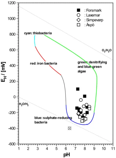
Figure 2 shows a plot of data obtained from the analyses by SKB of Swedish groundwaters at the sites Forsmark, Laxemar, Simevarp, and Aspö, and con-tained in a spreadsheet of abstracted data (Bath, 2008). The abstracted data are provided in Annex A, and, as can be seen, are incomplete. In selecting data from the database, preference was given to field data.

The Swedish ground waters are reducing (EH below 200 mV) and show

rather high pH. A single observation falls below the limits set by the stability of water with respect to H2 generation at 1 bar. This data point is for sample

KLX02/1560 at Laxemar. As in a larger number of cases, the EH value of

this sample is given in brackets in the provided database table.

A simple statistical analysis of all 35 reported EH values illustrates that they

together can be interpreted as one set being normally distributed with mean x = -207 mV and sigma s = 80 mV. The only value showing some clear devia-tion is the above mendevia-tioned Laxemar value at EH = -400 mV. This is shown

in Figure 3.

Fisher (1925), the founding father of scientific data analysis (Aldrich, 1997), provided a thorough basis for the analysis of experimental data. The task of analysing groundwater data is not much different from the task Fisher faced at Rothamsted Experimental Station in analysing agricultural data. Fisher, however, was able to suggest designed experiments to unravel the effects of various methods and treatments on plant growth (Fisher, 1935). The hydro-chemist / geologist is faced with a set of data that are unsuitable for ran-domisation. Nevertheless, modern data analysis tools allow an assessment of such data without reference to statistical models and assumptions on statisti-cal processes beyond maximum likelihood.

An example is given in Figure 4 where the EH-pH data provided by Bath

(2008) have been analysed by the robust minimum covariance determinant estimator (MCDE) (Rousseeuw and van Drissen, 1999). The MCDE at-tempts to interpret a given multivariate data set by a maximum likelihood

approach. The robustness is inferred from the breakdown level of 50 % for MCDE - the minimum value possible (implying maximum robustness). Thus, a model-free and robust classification tool like MCDE is a primary method of exploratory data analysis.

1 2 3 4 5 6 7 8 9 10 11 -600 -400 -200 0 200 400 600 800 1000 1200 : Forsmark : Laxemar : Simpevarp : Äspö blue: sulphate-reducing bacteria green: denitrifying and blue-green algae pH E H / [m V] H2O/H2 O2/H2O cyan: thiobacteria

red: iron bacteria

Figure 2: Oxidation-reduction potentials and associated pH pairs (n = 35)

for Swedish ground waters at sites Forsmark, Laxemar, Simpevarp, and Aspö in comparison with the limits of natural environments (cf. Fig. A-2, Appendix A).

-400 -300 -200 -100 0 100 0.0 0.2 0.4 0.6 0.8 1.0

: pooled EH data from Swedish ground waters

: closest fitting Normal distribution with x = -207 mV and s =80 mV (p=99.7 %) cu m ul at ive p ro ba bi lit y E_H / [mV]

Figure 3: Cumulative distribution of pooled 35 EH values of 35 ground

wa-ters from the four Swedish sites compared to the closest-fitting Normal dis-tribution with mean x = 207 mV and standard deviation s = 80 mV. The probability that the data are normally distributed and that the deviations are random is 99.7 %.

1 2 3 4 5 6 7 8 9 10 11 -600 -400 -200 0 200 400 600 800 1000 1200 : Forsmark : Laxemar : Simpevarp : Äspö blue: sulphate-reducing bacteria green: denitrifying and blue-green algae pH EH / [m V] H2O/H2 O2/H2O cyan: thiobacteria

red: iron bacteria

Figure 4: Interpretation of the reported EH-pH data pairs from Swedish

ground waters by robust minimum covariance determinant estimators (MCDE) (Rousseeuw and van Drissen, 1999) to assess associations between the data and to achieve an uncontaminated classification of the experimental data.

The breakdown level of a least-squares method refers to the number of out-liers (outlying observations, extraneous data, contamination). The classical least sum of squared residual methods (e.g. liner regression) suffers from the large effects outlying observations have on the resulting statistics, e.g., slope and intercept of a regression line (Meinrath and Schneider, 2007). This strong influence is also termed a ‘masking effect’, because the extraneous observations tend to shift the least squares estimators in a direction to in-clude the extraneous observation into the bulk of observations by: a) shifting the mean; and

b) increasing the variance.

Robust methods, e.g., the least median of squares estimator (Rousseeuw, 1993), are not sensitive to extraneous data up to a certain percentage. Hence, the estimators obtained by least squares regression have a breakdown level of 0 %, because one single outlying observation in a data set will shift the estimators. The "least median of squared residuals" estimator however, tol-erates up to 50 % of outlying observations. Up to this contamination level, the estimators are not shifted. Note that a higher breakdown level does not

make sense. If ‘contaminations’ make up more than half of the data the ques-tion arises: “Which contaminates which?” High-breakdown methods are increasingly being used in practice, e.g., in chemistry, process control, and finance (Meer et al., 1991; Rouesseeuw, 1997).

The set of pooled experimental data is interpreted by MCDE allowing for 50 % outlying observations. In the bivariate data space (pH and EH) a

variance-covariance ellipse is obtained enclosing the data points compatible with a similar (least-squares) mechanism.

Other data, showing large Mahalanobis1 distances under the minimum co-variance assumption, are subsequently interpreted excluding the already interpreted data. Thus, the EH-pH data of Swedish groundwaters are

classi-fied into two groups. The first group is given by the red ellipse, while the second group is centred about the blue ellipse. Two data points form their own (single member) groups: at (100 mV, pH 7.27) and at (-400 mV, pH 6.4). This classification is not based on any preliminary assumption except that the data are independent and represent random samples from a large population. This assumption corresponds to those underlying modern public polling strategies (Gallup, 1939).

Thus, the analysis indicates that the groundwater data are, despite the gaps in data, consistent. The presentation of the data, especially the large gaps and the pre-judgement of data (indicated, for instance, by bracketing some data), suggests that the data are not pure measurement data but have been edited according to some unknown criteria. It would be of importance to learn more about the editing criteria. On the basis of groundwater data analysis experi-ence during the past 20 years, the observation can be reported that EH

meas-urements, for a variety of rather subjective but virtually never objectified reasons, are often considered as ‘unreliable’ or ‘potentially contaminated’. The practical experience, however, indicates that EH values are usually no

less reliable than, e.g., ICP-AES data on groundwater samples when the resolution power of the equipment (usually ±30 mV) is taken into account. Even more than the 140 EH-pH data pairs measured in the groundwaters

sampled above the Gorleben salt dome between 1984 and 1989 (see Figure 5) could be nicely interpreted on the basis of the observations of Baas-Becking et al. (1960). In contrast to these waters with widely varying proper-ties (in terms of organic material content, ionic strength, sulphate/sulphide etc.), the Swedish low ionic strength granitic formation waters seem much more homogeneous. The preceding analysis advocates trusting the measure-ments and interpreting the data only after a thorough data analysis. To illus-trate this point, the following figure shows data collected during German uranium mining remediation activities of former East German-Soviet com-pany WISMUT.

The few data points in Figure 5 at low pH falling outside the limits of natural aqueous systems are due to in-situ sulphuric acid leaching (Königstein sand-stone mine). These conditions are definitively non-natural. All data were

1 _{The Mahalanobis distance is based on correlations between variables from which different patterns can be}

collected during work on diploma theses or doctoral work by researchers generally unaware of the work of Baas-Becking et al. (1960).

UO22+(aq) UO2(CO3)3 4-U4+ U3+ UCO32+ U (C O3 )2 U(CO3)3 2-U (C O3 )4 4-carbonato species/UO2+ 1 2 3 4 5 6 7 8 9 10 11 12 13 pH U O2 C O3 -1.0 -0.8 -0.6 -0.4 -0.2 0.0 0.2 0.4 0.6 0.8 1.2 1.0 1.4 U(OH)4/UO2+ -19 -15 -10lg [CO3-5 -1 2-_] 0.03 kPa CO2 O_2/H 2O

: sandstone deposit; sulfuric acid leached [14] : mill tailings 1; (this work)

: mill tailings 2; (this work)

: control well; unaffected by uranium mining [14]

: unaffected groundwater from Turonian sandstone formation

re do x po te nt ia l EH / [V ] U(CO3)5 6-H_2O/H 2

Figure 5: Field data from three different sites contaminated by former

min-ing activities and (unaffected) control wells in Saxonia, Germany. The data are compared to the limits of natural aqueous environments (Baas-Becking et al., 1960) and the redox boundaries of uranium. Further details are given in Meinrath et al. (1999).

5.2 Carbonate in Groundwaters

CO2 in the air dissolves in water forming successively HCO3

and CO3

2-. These processes can be described in terms of chemical equilibria:

and

lg[CO

]  lg (K

K

K

)  lg pCO

 2 pH

The constants KH, K1 and K2 are the Henry constant for dissolution of gase-ous CO2 in an aqueous medium, the first dissociation constant of H2CO3, and

the second dissociation constant of H2CO3, respectively. These constants

vary with ionic strength and temperature of an aqueous medium. However, under ambient conditions the variations in pH and pCO2, the partial pressure

of CO2, are larger than those observed in KH, K1 and K2. Thus by correlating

pH with lg [HCO3-], some conclusions can be obtained on pCO2 for a given

water. The ambient CO2 partial pressure is about 0.0316 %.

pCO2 in groundwaters is greater than that in the atmosphere as a result of

production of CO2 by plant roots. Due to this source, pCO2 in soil from the first 20 cm below surface may reach up to 20 %. Meteoritic water percolat-ing these soil layers saturates with CO2 durpercolat-ing ground water recharge. Mi-crobially-mediated degradation of organic matter may also contribute addi-tional CO2. Consequently, pCO2 in groundwaters may reach 10 % in

groundwater.

Figure 6 shows the results from the analysis of a number of groundwaters, with data pairs for pH and lg [HCO3] interpreted in terms of pCO2. The data

were collected routinely by four different groups who were unaware of this type of correlation at the time of data collection. Nevertheless, no data points fall below the lower line representing atmospheric CO2 partial pressure, with

-1

-2

-3

-4

-5

pH

lg

[H

C

O

]

3

-9

8

7

6

5

Figure 6: Correlation of measured HCO3

concentrations with measured pH and pCO2. Experimental data from four continents are given representing a

wide variety of conditions including about 140 data pairs from the formation above the Gorleben site.

5.3 Swedish Groundwaters: pH vs. lg [HCO3-_]

Figure 7 shows a similar plot to that of Figure 6, but with data included for groundwaters collected from four sites in Sweden. Given the data presented in Figure 6, the observations made for the Swedish groundwaters are differ-ent in the respect that most of the data for all four sites fall below the limit of atmospheric CO2 partial pressure. This may be the result of calcium release

and proton consumption from aluminosilicate alteration in the deep bedrock (isolated from equilibration with atmospheric CO2). Consequently, the

re-sulting calcite precipitation will remove inorganic carbon from solution. Moreover, deep saline groundwater tend to have high concentrations of Ca2+ and more calcite is allowed to precipitate, which results in pH increases and [HCO3 -] reductions.

-1

-2

-3

-4

-5

pH

lg

[HCO

]

3

-9

8

7

6

5

Gorleben/Europe

NT/Australia

Tanzania/Africa

Snow Lake/Canada

Figure 7: Correlation of measured HCO3- concentrations with measured pH

and pCO2. Experimental data from four continents are compared to the data

6. Data Reliability and

GUM-Compliant

Uncer-tainty Assessment of

Sorption Data

In the context of good laboratory practice, the basis for the development of the international consensus document “Guide to the Expression of

Uncer-tainty in Measurement” (GUM) is discussed in Appendix B together with the

basic steps in the underlying procedure. Here, the GUM approach is applied to an uncertainty assessment of sorption data.

6.1 Sorption

6.1.1 Process

Within performance assessment of nuclear waste repositories, sorption plays an important role as a fundamental retardation process. Retardation may be quantitatively expressed by the (dimensionless) retardation coefficient Rf:

R

 1 

K





(eq. 1)

where

 = density of stationary phase (kg/m3), formation = porosity [-],

Kd = sorption or distribution coefficient (m3/kg). Despite extensive work being carried out to demonstrate the basis for more complex surface sorption models to be reliable predictors of retardation, the simple Kd model still dominates in nuclear waste repository performance assessment. K_d  Csorb [C_sol] V_t m (eq.2) where

Csorb = amount of A sorbed on the solid matrix [moles];

[Csol] = amount of of A in solution [moles];

Vt = volume of solution [dm3];

6.1.2 Uncertainty Analysis of Experimental Sorption Data

Equation (2) was used in the analysis of experimentally obtained data for the evaluation of a Kd value for the sorption of a radionuclide on granite

(Andersson et al., 2008). The associated data in the report are accompanied by explanatory text indicating that the uncertainty analysis was not under-taken according to international consensus but following an individual pro-cedure. The text from Andersson et al. (2008) describing the determination of the error associated with Rd, the experimental measurement of Kd, is pro-vided in Annex B. For convenience, the final equation derived for the error on Rd is provided below.





(eq.4-25) from Andersson et al. (2008; see also Annex B).

Using this experimental work as an example, this section describes how the data and information provided in Anderssson et al. (2008) have been adapted to the international consensus GUM-compliant approach together with a brief discussion of the results.

In terms of constraints associated with this exercise, numerical values were not given in the text but provided on a separate worksheet. From this work-sheet, the radioactive tracer was identified as 152Eu. The concentration of the carrier was 6.4E07 M.

Based on eq. 4-25 in Andersson et al. (2008), an 'effective cause-and-effect diagram' can be derived, as shown in Figure 8, and the influence factors are included in Table 1. Note that Table 1 also contains those influence factors mentioned in the text but not further discussed.

Table 1: Influence factors considered in the evaluation of an Rd value for 152

Eu to Kivetty granite (0.045 mm – 2 mm fraction) in Olkiluoto saline wa-ter at pH 8.5.

Influence factor Symbol u 

Activity concentration of tracer1) C 1

Accumulated withdrawals of activity by n repeated samplings

Autt,n 1

Product of wall sorption coefficient Rd,ref and "wall

mass mw"

Ld 1

Sum of withdrawn activity



A

Atot, ref Atot, ref ?

Hydroxide concentration [OH] ?

Ligand concentration [L] ?

Background --- --- ---

1

Note: C is used for two quantities: the tracer concentration in the reference (unfor-tunately a mean concentration is used; cf. eq. 4-11 in Annex B), and the concentra-tion in the tracer stock soluconcentra-tion (cf. eq. 4-12 in Annex B).

In addition to the influence factors summarized above the "experimental

limitation where the amount of adsorbed material is measured indirectly, by measuring what is left in solution und using the mass balance" is mentioned

without further recurrence to this crucial step in the uncertainty assessment of a Kd value.

R

Figure 8: Approximate cause-and-effect diagram for the evaluation of Rd

values for the sorption of 152Eu to Kivetty granite (0.045 mm – 2 mm frac-tion) in Olkiluoto saline water at pH 8.5.

The extracted text in Andersson et al. (2008; see Annex B) is rather difficult to follow from a quality assurance (QA) perspective. The motivation behind the individual steps is mostly hidden and the summary error (in Rd) in eq. 4-25 (Annex B) is almost untrackable.

The researchers were faced with the same three tasks mentioned in the intro-duction to Appendix B:

 The need for extensive documentation of the individual steps.  Keeping track of various systematic and random uncertainty

contributions (in fact, the discussion either does not address the respective contributions, or ascertains that the magnitude of the variability is negligible, or urges caution instead of presenting a repeatability or reproducibility.

 Finding a suitable compromise between the quest for conserva-tisms and the need to have small overall uncertainties.

The abstracted text in Annex B, therefore, highlights the need for an interna-tionally-accepted convention to communicate on measurement uncertainty as is provided by the GUM and supplemented by the various guides from EURACHEM (2000, 2002).

To emphasise this point, reference is made to the first equation defining the

Rd, the quantity of interest. In this case, Asorb, the activity sorbed on the solid, must be evaluated from the difference between two other quantities, quanti-ties, Aaq (the activity of radionuclide in the aqueous phase) and Atot (total amount of radionuclide added initially), both of which are affected by uncer-tainty. Hence, a term like

Asorb = (Atot - Aaq) (eq. 3)

may be expected. Subsequently

m A V A A R aq aq tot d ) (   (eq. 4)

Note that the evaluation of Rd in eq.4-25 (Annex B) is not applicable for error propagation involving product or quotient operations.

Furthermore, the (unspecified) concentration of the carrier plays an impor-tant role because Eu(III) is a rather insoluble compound at pH 8.5. Eu(III) hydrolyses and coordinates to carbonate. In assessing the solution conditions for this hydrolysable ion, the presence of 'saline water' as solution phase should be mentioned. Hence, there are additional issues in estimating a rea-sonable solution pH. Commercially available traceable pH calibration buff-ers are valid up to an ionic strength I = 0.3 mol only. The ratio of inactive Eu to 152Eu sets a limitation on the total activity to be added to the sample. Hence, the information provided is not sufficient to judge the respective data. The initial activity of 152Eu, Atot, is not given. Consequently the

com-plete analysis cannot be retraced. However, the rather sensitive relationship among the different activity contributions in Eqs. 3 and 4 can be addressed. Three situations can be assumed:

a) low sorption tendency: Aaq ~ Atot

b) high sorption tendency: Atot ~ (Atot - Aaq)

c) intermediate sorption tendency: Aaq ~ (Atot - Aaq)

In case a) the measurement uncertainty is crucially dependent on the count-ing uncertainties in Aaq and Atot because the quantity of interest, Asorb, is ob-tained as the small difference between two large numbers. In some situations even negative differences may result. This situation should have been ob-served in the case of the wall sorption study component of the experimental work under review here.

In case b) the count rate in the aqueous phase is very small and, hence, close to background activity. Background counting variations cannot be neglected - and even determine the final result.

Situation c) is the most appropriate where the activity divides equally be-tween the sorbed and the aqueous state. This situation can be adjusted within rather narrow limits by fixing the ratio V:m. However, because these

amounts usually cannot be varied over orders of magnitude, the experimental conditions are mostly determined by the system under study. A lump treat-ment of measuretreat-ment uncertainties for Kd values ("...are in the order of...") is therefore inappropriate. 0 50 100 150 200 0 1000 2000 3000 4000 5000 6000 25000 30000 sorption of 152_Eu wall01 wall02 batch01 batch02 acidic co un ts p er m in ut e time / [days]

Figure 9: Experimental data on 152Eu sorption on Kivetty granite (0.045 mm